Training Tree Transducers

Jonathan Graehl

University of Southern California

Kevin Knight

University of Southern California

Jonathan May

University of Southern California

Many probabilistic models for natural language are now written in terms of hierarchical tree structure. Tree-based modeling still lacks many of the standard tools taken for granted in (finite-state) string-based modeling. The theory of tree transducer automata provides a possible framework to draw on, as it has been worked out in an extensive literature. We motivate the use of tree transducers for natural language and address the training problem for probabilistic tree-to-tree and tree-to-string transducers.

1. Introduction

Much natural language work over the past decade has employed probabilistic finite-state transducers (FSTs) operating on strings. This has occurred somewhat under the influence of speech recognition research, where transducing acoustic sequences to word sequences is neatly captured by left-to-right stateful substitution. Many conceptual tools exist, such as Viterbi decoding (Viterbi 1967) and forward–backward training (Baum and Eagon 1967), as well as software toolkits like the AT&T FSM Library and USC/ISI’s Carmel.1 Moreover, a surprising variety of problems are attackable with FSTs, from part-of-speech tagging to letter-to-sound conversion to name transliteration.

However, language problems like machine translation break this mold, because they involve massive re-ordering of symbols, and because the transformation processes seem sensitive to hierarchical tree structure. Recently, specific probabilistic tree-based models have been proposed not only for machine translation (Wu 1997; Alshawi, Bangalore, and Douglas 2000; Yamada and Knight 2001; Eisner 2003; Gildea 2003), but also for summarization (Knight and Marcu 2002), paraphrasing (Pang, Knight, and Marcu 2003), natural language generation (Langkilde and Knight 1998; Bangalore and Rambow 2000; Corston-Oliver et al. 2002), parsing, and language modeling (Baker 1979; Lari and Young 1990; Collins 1997; Chelba and Jelinek 2000; Charniak 2001; Klein

∗Information Sciences Institute, 4676 Admiralty Way, Marina del Rey, CA 90292. E-mail: [email protected]. ∗∗Information Sciences Institute, 4676 Admiralty Way, Marina del Rey, CA 90292. E-mail: [email protected]. †Information Sciences Institute, 4676 Admiralty Way, Marina del Rey, CA 90292. E-mail: [email protected]. 1www.research.att.com/sw/tools/fsm and www.isi.edu/licensed-sw/carmel.

and Manning 2003). It is useful to understand generic algorithms that may support all these tasks and more.

Rounds (1970) and Thatcher (1970) independently introduced tree transducers as a generalization of FSTs. Rounds was motivated by natural language:

Recent developments in the theory of automata have pointed to an extension of the domain of definition of automata from strings to trees . . . parts of mathematical linguistics can be formalized easily in a tree-automaton setting . . . We investigate decision problems and closure properties. Our results should clarify the nature of syntax-directed translations and transformational grammars . . . (Rounds 1970)

The Rounds/Thatcher tree transducer is very similar to a left-to-right FST, except that it works top-down, pursuing subtrees independently, with each subtree transformed depending only on its own passed-down state. This class of transducer, called R in earlier works (Gécseg and Steinby 1984; Graehl and Knight 2004) for “root-to-frontier,” is often nowadays called T, for “top-down”.

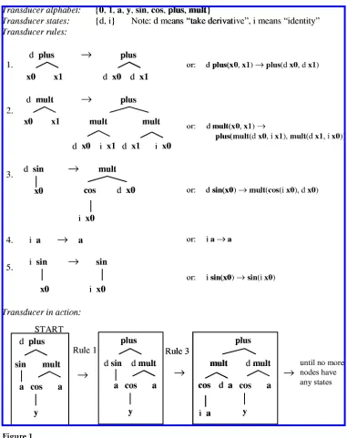
Rounds uses a mathematics-oriented example of a T transducer, which we repeat in Figure 1. At each point in the top-down traversal, the transducer chooses a produc-tion to apply, basedonlyon the current state and the current root symbol. The traversal continues until there are no more state-annotated nodes. Non-deterministic transducers may have several productions with the same left-hand side, and therefore some free choices to make during transduction.

A T transducer compactly represents a potentially infinite set of input/output tree pairs: exactly those pairs (T1, T2) for which some sequence of productions applied to T1 (starting in the initial state) results in T2. This is similar to an FST, which compactly represents a set of input/output string pairs; in fact, T is a generalization of FST. If we think of strings written down vertically, as degenerate trees, we can convert any FST into a T transducer by automatically replacing FST transitions with T produc-tions, as follows: If an FST transition from state q to state r reads input symbol A and outputs symbol B, then the corresponding T production is q A(x0) → B(r x0). If the FST transition output is epsilon, then we have instead q A(x0) → r x0, or if the input is epsilon, then q x0→B(r x0). Figure 2 depicts a sample FST and its equivalent T transducer.

T does have some extra power beyond path following and state-based record-keeping. It can copy whole subtrees, and transform those subtrees differently. It can also delete subtrees without inspecting them (imagine by analogy an FST that quits and accepts right in the middle of an input string). Variants of T that disallow copying and deleting are called LT (forlinear) and NT (fornondeleting), respectively.

One advantage to working with tree transducers is the large and useful body of literature about these automata; two excellent surveys are Gécseg and Steinby (1984) and Comon et al. (1997). For example, it is known that T is not closed under composition (Rounds 1970), and neither are LT or B (the “bottom-up” cousin of T), but the non-copying LB is closed under composition. Many of these composition results are first found in Engelfriet (1975).

Figure 1

Part of a sample T tree transducer, adapted from Rounds (1970).

consists only of q S(x0, x1), although we want the English-to-Arabic transformation to apply only when it faces the entire structure q S(PRO, VP(V, NP)). However, we can simulate lookahead using states, as in these productions:

q S(x0, x1)→ S(qpro x0, qvp.v.np x1) qpro PRO→ PRO

Figure 2

An FST and its equivalent T transducer.

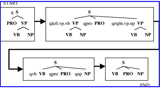
By omitting rules like qpro NP→..., we ensure that the entire production sequence will dead-end unless the first child of the input tree is in fact PRO. So finite lookahead (into inputs we don’t delete) is not a problem. But these productions do not actually move the subtrees around. The next problem is how to get the PRO to appear between the V and NP, as in Arabic. This can be carried out using copying. We make two copies of the English VP, and assign them different states, as in the following productions. States encode instructions for extracting/positioning the relevant portions of the VP. For example, the state qleft.vp.v means “assuming this tree is a VP whose left child is V, output only the V, and delete the right child”:

q S(x0, x1)→ S(qleft.vp.v x1, qpro x0, qright.vp.np x1) qpro PRO→ PRO

qleft.vp.v VP(x0, x1)→ qv x0 qright.vp.np VP(x0, x1)→ qnp x1

With these rules, the transduction proceeds as in Figure 3. This ends our informal pre-sentation of tree transducers.

Figure 3

Multilevel re-ordering of nodes in a T-transducer.

with rules R, and (2) a finite training set of sample input/output tree pairs, we want to produce (3) a probability estimate for each rule in R such that we maximize the probability of the output trees given the input trees. As with the forward–backward algorithm, we seek at least a local maximum. Tree transducers with weights have been studied (Kuich 1999; Engelfriet, Fülöp, and Vogler 2004; Fülöp and Vogler 2004) but we know of no existing training procedure.

Sections 2–4 of this article define basic concepts and recall the notions of relevant au-tomata and grammars. Sections 5–7 describe a novel tree transducer training algorithm, and Sections 8–10 describe a variant of that training algorithm for trees and strings. Section 11 presents an example linguistic tree transducer and provides empirical evi-dence of the feasibility of the training algorithm. Section 12 describes how the training algorithm may be used for training context-free grammars. Section 13 discusses related and future work.

2. Trees

TΣis the set of(rooted, ordered, labeled, finite) trees over alphabetΣ.Analphabetis a finite

set. (see Table 1)

TΣ(X) are the trees over alphabetΣ, indexed by X—the subset ofTΣ∪X where only

leaves may be labeled byX(TΣ(∅)=TΣ).Leavesare nodes with no children.

Thenodesof a treetare identified one-to-one with itspaths:paths_t⊂paths≡N∗≡

∞

i=0N

i _(N0_{≡ {()}). The size of a tree is the number of nodes: |t|=|pathst|. The path}

to the root is the empty sequence (), and p₁ extended by p₂ is p₁·p₂, where · is the concatenation operator:

(a1,. . .,an)·(b1,. . .,bm)≡(a1,. . .,an,b1,. . .,bm)

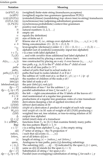
Table 1

Notation guide.

Notation Meaning

(w)FS(T,A) (weighted) finite-state string (transducers,acceptors) (w)RTG (weighted) regular tree grammars (generalizes PCFG)

(x)(L)(N)T(s) (extended) (linear) (nondeleting) top–down tree(-to-string) transducers (S)T(A,S)G (synchronous) tree (adjoining,substitution) grammars

(S,P)CFG (synchronous,probabilistic) context-free grammars

R+

positive real numbers

N natural numbers: {1, 2, 3,. . .} ∅ empty set

≡ equals (by definition) |A| size of finite setA

X∗ Kleene star ofX, i.e., strings over alphabetX:{(x1,. . .,xn)|n≥0}

a·b String concatenation: (1)·(2, 3)=(1, 2, 3)

<lex lexicographic (dictionary) order: ()<(1)<(1, 1)< . . . <(1, 2)< . . .

Σ alphabet (set of symbols) (commonly: input tree alphabet)

t∈TΣ tis a tree with label alphabetΣ

TΣ(X) ... and withvariablesfrom additional leaf label alphabetX A(t) tree constructed by placing a unaryAabove treet

A((x1,. . .,xn)) tree constructed by placing ann-aryAover leaves (x1,. . .,xn)

p tree path, e.g., (a,b) is thebth_{child of thea}th_{child of root}

paths the set of all tree paths (≡N∗)

paths_t subset ofpathsthat lead to actual nodes int paths_t({A,B}) paths that lead to nodes labeledAorBint

t↓p the subtree oftwith root atp, so that (t↓p)↓q=t↓(p·q)

rankt(p) the number of children of the nodepoft

labelt(p) the label of nodepoft

labelandrankt(p) the pair (labelt(p),rankt(p))

t[p←t] substitution of treetfor the subtreet↓p t[p←tp,∀p∈P] parallel substitution of treetpfor eacht↓p

yield_t(X) the left→right concatenation of theXlabels of the leaves oft S∈N start nonterminal of a regular tree grammar

P,R productions of a regular tree grammar, rules of a tree transducer

D(M) derivations (keeping a list of applied rewrites) ofM LD(M) leftmostderivations ofM

wM(d∈D(M)) weightof a derivationd: product of weight of each rule usage

WM(x) total weightofxinM: sum of weight of allLD(M) producingx

L(M) weighted tree set, tree relation, or tree-to-string relation ofM ∆ output tree alphabet

Qi∈Q initial (start) state of a transducer

λ∈xTPATΣ functions fromTΣto{0, 1}that examine finitely many paths True the tree patternTrue(t)≡1,∀t

s∈Σ∗ sis a string from alphabetΣ, e.g., () the empty string

s[i] ithletter of string s - theith projectionπi

indicess isuch thats[i] exists: (1,. . .,|s|)

letterss set of all letterss[i] ins

|s| length of string;|s|=|indicess|,not|letterss|

spans_s Analogous to tree paths, pairs (i,j) denoting substrings

s↓(i,j) The substring (s[i],. . .,s[j−1]) indicated by the span (i,j)∈spans_s s↓[i] same ass[i]; [i] stands for the span (i,i+1)

s[p←s] Substitution of stringsfor spanpofs

path p·(i). Thesubtree at path p of tist↓p, defined bypaths_t↓p≡ {q|p·q∈pathst}and labelandrank_t↓p(q)≡labelandrankt(p·q).

Thepaths to X in tarepaths_t(X)≡ {p∈pathst|labelt(p)∈X}.

A set of pathsF⊂pathsis afrontieriff it ispairwise prefix-independent:

∀p1,p2∈F,p∈paths:p1=p2·p =⇒ p1=p2

We writeFfor the set of all frontiers.Fis afrontier of t, ifF⊂Ftis a frontier whose paths are all valid fort—Ft≡F∩pathst.

Fort,s∈TΣ(X),p∈paths_t,t[p←s] is thesubstitution of s for pint, where the subtree

at pathpis replaced bys. For a frontierFoft, theparallel substitution of t_pfor the frontier F∈Ftin tis writtent[p←tp,∀p∈F], where there is atp∈TΣ(X) for each pathp. The

result of a parallel substitution is the composition of the serial substitutions for allp∈F, replacing eacht↓pwitht_p. ( IfFwere not a frontier, the result would vary with the order of substitutions sharing a common prefix.) For example:t[p←t↓p·(1),∀p∈F] would splice out each nodep∈F, replacing it by its first subtree.

Trees may be written as strings overΣ∪ {( , )}in the usual way. For example, the tree t=S(NP, VP(V, NP)) has labelandrank_t((2))=(VP, 2) and labelandrank_t((2, 1))=(V, 0). Commas, written only to separate symbols in Σ composed of several typographic letters, should not be considered part of the string. For example, if we write σ(t) for σ∈Σ,t∈TΣ, we mean the tree withlabelσ(t)(())≡σ,rankσ(t)(())≡1 andσ(t)↓(1)≡t.

Using this notation, we can give a definition ofTΣ(X):

Ifx∈X, thenx∈TΣ(X) ( 1)

Ifσ∈Σ, thenσ∈TΣ(X) ( 2)

Ifσ∈Σandt₁,. . .,t_n∈TΣ(X), thenσ(t1,. . .,tn)∈TΣ(X) ( 3)

Theyield of X in tisyield_t(X), the concatenation (in lexicographic order2) over paths to leavesl∈paths_t(such thatrankt(l)=0) oflabelt(l)∈X—that is, the string formed by reading out the leaves labeled withXin left-to-right order. The usual case (theyield of t) isyield_t≡yield_t(Σ). More precisely,

yield_t(X)≡   

l ifr=0∧l∈Xwhere (l,r)≡labelandrankt(())

( ) ifr=0∧l∈X

•r

i=1yieldt↓(i)(X) otherwise where• r

i=1si≡s1·. . .·sr

3. Regular Tree Grammars

In this section, we describe the regular tree grammar, a common way of compactly representing a potentially infinite set of trees (similar to the role played by the regu-lar grammar for strings). We describe the version where trees in a set have different weights, in the same way that a weighted finite-state acceptor gives weights for strings

Σ={S, NP, VP, PP, PREP, DET, N, V, run, the, of, sons, daughters} N ={qnp, qpp, qdet, qn, qprep}

S = q

P ={q→1.0S(qnp, VP(VB(run))), qnp→0.6NP(qdet, qn), qnp→0.4NP(qnp, qpp), qpp→1.0PP(qprep, np), qdet→1.0DET(the), qprep→1.0PREP(of), qn→0.5N(sons), qn→0.5N(daughters)}

Sample generated trees:

S(NP(DT(the), N(sons)), VP(V(run)))

(with probability 0.3)

S(NP(NP(DT(the), N(sons)),

PP(PREP(of), NP(DT(the), N(daughters)))), VP(V(run)))

(with probability 0.036)

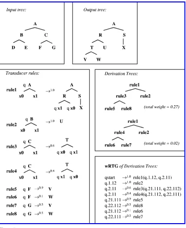
Figure 4

A sample weighted regular tree grammar (wRTG).

in a regular language; when discussing weights, we assume the commutative semiring ({r∈R|r≥0},+,·, 0, 1) of nonnegative reals with the usual sum and product.

Aweighted regular tree grammar(wRTG)Gis a quadruple (Σ,N,S,P), whereΣis the alphabet,Nis the finite set ofnonterminals,S∈Nis thestart (or initial) nonterminal, andP⊆N×TΣ(N)×R

+

is a finite set ofweighted productions(R+≡ {r∈R|r>0}). A production (lhs,rhs,w) is writtenlhs→wrhs(ifwis omitted, the multiplicative identity 1 is assumed). Productions whoserhs contains no nonterminals (rhs∈TΣ) are called terminal productions, and rules of the formA→wB, forA,B∈Nare called-productions, orstate-change productions, and can be used in lieu of multiple initial nonterminals.

Figure 4 shows a sample wRTG. This grammar generates an infinite number of trees. We define the binary derivation relation on terms TΣ(N) and derivationhistories

(TΣ(N×(paths×P)∗):

⇒G≡

((a,h), (b,h·(p, (l,r,w))))|(l,r,w)∈P∧

p∈paths_a({l})∧

That is, (a,h)⇒G(b,h·(p, (l,r,w))) iffb may be derived from aby using the rule l→wrto replace the nonterminal leaflat pathpwithr. The reflexive, transitive closure of ⇒G is written ⇒∗_G, and the derivations of G, written D(G), are the ways the start nonterminal may be expanded into entirely terminal trees:

D(G)≡

(t,h)∈TΣ×(paths×P)∗|(S, ( ))⇒∗G(t,h)

We also project the ⇒∗_G relation so that it refers only to trees: t⇒_G∗t iff ∃h,h∈ (paths×P)∗: (t,h)⇒∗_G(t,h).

We take the product of the used weights to get theweight of a derivation d∈D(G):

wG((t, (h1,. . .,hn))∈D(G))≡ n

i=1

wiwherehi=(pi, (li,ri,wi))

Theleftmost derivations of Gbuild a tree preorder from left to right (always expand-ing the leftmost nonterminal in its strexpand-ing representation):

LD(G)≡

(t, ( (p1,r1),. . ., (pn,rn)))∈DG| ∀1≤i<n:pi+1≮lexpi

Thetotal weight of t in Gis given byWG:TΣ→R, the sum of the weights of leftmost

derivations producing t:WG(t)≡

(t,h)∈LD(G)wG((t,h)). Collecting the total weight of every possible (nonzero weight) output tree, we callL(G) theweighted tree languageof G, whereL(G)={(t,w)|WG(t)=w∧w>0}(the unweighted tree language is simply the first projection).

For every weighted context-free grammar, there is an equivalent wRTG that gener-ates its weighted derivation trees (whose yield is a string in the context-free language), and the yield of any regular tree language is a context-free string language (Gécseg and Steinby 1984). We can also interpret a regular tree grammar as a context-free string grammar with alphabetΣ∪ {( , )}.

wRTGs generate (ignoring weights) exactly the recognizable tree languages, which are sets of trees accepted by a non-transducing automaton version of T. This acceptor automaton is described in Doner (1970) and is actually a closer mechanical analogue to an FSA than is the rewrite-rule-based wRTG. RTGs are closed under intersection (Gécseg and Steinby 1984), and the constructive proof also applies to weighted wRTG intersection. There is a normal form for wRTGs analogous to that of regular grammars: Right-hand sides are a single terminal root with (optional) nonterminal children. What is sometimes called aforestin natural language generation (Langkilde 2000; Nederhof and Satta 2002) is a finite wRTG without loops—for all valid derivation trees, each nonterminal may only occur once in any path from root to a leaf:

∀n∈N,t∈TΣ(N),h∈(paths×P)∗: (n, ( ))⇒∗G(t,h) =⇒ pathst({n})=∅

and their adjunction operation; the productions correspond exactly to TAG’s initial trees and the elementary tree substitution operation.

4. Extended-LHS Tree Transducers (xT)

Section 1 informally described the root-to-frontier transducer class T. We saw that T allows, by use of states, finite lookahead and arbitrary rearrangement of non-sibling input subtrees removed by a finite distance. However, it is often easier to write rules that explicitly represent such lookahead and movement, relieving the burden on the user to produce the requisite intermediary rules and states. We define xT, a generalization of weighted T. Because of its good fit to natural language problems, xT is already briefly touched on, though not defined, in Section 4 of Rounds (1970).

A weighted extended-lhs top-down tree transducer M is a quintuple (Σ,∆,Q,Qi,R) whereΣis the input alphabet, and∆is the output alphabet,Qis a finite set of states, Qi∈Qis theinitial (or start, or root) state, andR⊆Q×xTPATΣ×T∆(Q×paths)×R+

is a finite set of weighted transformation rules. xTPATΣ is the set of finite tree patterns:

predicate functions f :TΣ→ {0, 1}that depend only on the label and rank of a finite

number of fixed paths of their input. A rule (q,λ,rhs,w) is written qλ→w rhs, mean-ing that an input subtree matchmean-ing λ while in state q is transformed into rhs, with Q×pathsleaves replaced by their (recursive) transformations. TheQ×pathsleaves of a rhsare callednonterminals(there may also beterminalleaves labeled by the output tree alphabet∆).

xT is the set of all such transducers T; the set of conventional top-down trans-ducers, is a subset of xT where the rules are restricted to use finite tree patterns that de-pend only on the root:TPATΣ≡ {pσ,r(t)}wherepσ,r(t)≡(labelt(())=σ∧rankt(())=r). Rules whoserhsare a pureT∆with no states/paths for further expansion are called terminal rules. Rules of the form qλ →w q( ) are -rules, or state-change rules, which substitute stateq for stateqwithout producing output, and stay at the current input subtree. Multiple initial states are not needed: we can use a single start stateQi, and instead of each initial stateqwith starting weightwadd the ruleQiTrue→wq() (where True(t)≡1,∀t).

We define the binary derivation relation for xT transducer M on partially trans-formed terms and derivation historiesTΣ∪∆∪Q×(paths×R)∗:

⇒M≡

((a,h), (b,h·(i, (q,λ,rhs,w))))|(q,λ,rhs,w)∈R∧

i∈paths_a∧q=labela(i)∧λ(a↓(i·(1)))=1∧

b=a

i←rhs

p←q(a↓(i·(1)·i)), ∀p∈paths_rhs:labelrhs(p)=(q,i)

That is,bis derived fromaby application of a rule qλ→wrhsto an unprocessed input subtreea↓iwhich is in stateq, replacing it by output given byrhswith variables (q,i) replaced by the input subtree at relative pathiin stateq.3

Let⇒∗_M,D(M),LD(M),wM,WM, andL(M) ( theweighted tree relationofM) follow from the single-step⇒Mexactly as they did in Section 3, except that the arguments are

input and output instead of just output, with initial termsQi(t) for each inputt∈TΣin

place ofS:

D(M)≡

(t,t,h)∈TΣ×T∆×(paths×R)∗|(Qi(t), ())⇒∗M(t _,h)

We have given a rewrite semantics for our transducer, similar to wRTG. In the intermediate terms of a derivation, the active frontier of computation moves top-down, with everything above that frontier forming the top portion of the final output. The next rewrite always occurs somewhere on the frontier, and in acomplete derivation, the frontier finally shrinks and disappears. In wRTG, the frontier consisted of the nonterminal-labeled leaves. In xT, the frontier items are not nonterminals, but pairs of state and input subtrees. We choose to represent these pairs as subtrees of terms with labels taken from Σ∪∆∪Q, where the state is the parent of the input subtree. In fact, given anM∈xT and an input treet, we can take all the (finitely many) pairs of input subtrees and states as nonterminals in a wRTGG, with all the (finitely many) possible single-step derivation rewrites ofMapplied totas productions (taking the weight of the xT rule used), and the initial termQi(t) as the start nonterminal, isomorphic to the derivations of theMwhich start withQi(t): (d,h)∈D(G) iff (t,d,h)∈D(M). Such derivations are exactly how all the outputs of an input treetare produced: when the resulting termdis inT∆, we say that

(t,d) is in the tree relation and thatdis an output oft.

Naturally, there may be input trees for which no complete derivation exists—such inputs are not in the domain of the weighted tree relation, having no output. It is known thatdomain(M)≡ {i| ∃o,w: (i,o,w)∈L(M)}, the set of inputs that produce any output, is always a recognizable tree language (Rounds 1970).

Thesourcesof a ruler=(q,l,rhs,w)∈Rare the input-paths in therhs:

sources(r)≡ {i| ∃p∈paths_rhs(Q×paths),q∈Q:labelrhs(p)=(q,i)}

If the sources of a rule refer to input paths that do not exist in the input, then the rule cannot apply (becausea↓(i·(1)·i) would not exist). In the traditional statement of T, sources(r) are the variables xi, standing for the ith child of the root at path (i), and the right hand sides of rules refer to them by name: (qi,xi). In xT, however, we refer to the mapped input subtrees by path (and we are not limited to the immediate children of the root of the subtree under transformation, but may choose any frontier of it).

A transducer islinearif for all its rulesr,sources(r) are a frontier and occur at most once:∀p₁,p₂∈paths_rhs(Q×paths),p∈paths− {()}:p₁ =p₂·p. A transducer is determin-isticif for any input, at most one rule matches per state:

∀q∈Q,t∈TΣ,r=(q,p,r,w),r=(q,p,r,w)∈R: p(t)=1∧p(t)=1 =⇒ r=r

or in other words, the rules for a given state have patterns that partition possible input trees. A transducer is deleting if there are rules in which (for some matching inputs) entire subtrees are not used in theirrhs.

variables in therhsinstead of writing the corresponding path in thelhs. For example: q A(x0:B,C) →w qx0means a xT rule (q,λ,rhs,w) withrhs=(q, ( 1)) and

λ≡(labelandrank_t(())=(A, 1)∧label_t((1))=B∧labelandrank_t((2))=(C, 0))

It might be convenient to convert any xT transducer to an equivalent T transducer, then process it with T-based algorithms—in such a case, xT would just be syntactic sugar for T. We can automatically generate T productions that use extra states to emulate the finite lookahead and movement available in xT (as demonstrated in Section 1), but with one fatal flaw: Because of the definition of ⇒M, xT (and thus T) only has the ability to process input subtrees that produce corresponding output subtrees (alas, there is no such thing as an empty tree), and becauseTPATcan only inspect the root node while deriving replacement subtrees, T can check only the parts of the input subtree that lie along paths that are referenced in therhsof the xT rule. For example, suppose we want to transform NP(DET, N) (but not, say, NP(ADJ, N)) into the tree N using rules in T. Although this is a simple xT rule, the closest we can get with T would be q NP(x0, x1) →q.N x1, but we cannot check both subtrees without emitting two independent subtrees in the output (which rules out producing just N). Thus, xT is a bit more powerful than T.

5. Parsing an xT Tree Relation

Derivation trees for a transducer M=(Σ,∆,Q,Qi,R) are TR (trees labeled by rules) isomorphic to complete leftmost M-derivations. Figure 5 shows derivation trees for a particular transducer. In order to generate derivation trees forMautomatically, we build a modified transducerM. This new transducer produces derivation trees on its output instead of normal output trees.Mis (Σ,R,Q,Qi,R), with4

R≡ {(q,λ,r(yield_rhs(Q×paths)),w)|r=(q,λ,rhs,w)∈R}

That is, the originalrhsof rules are flattened into a tree of depth 1, with the root labeled by the original rule, and all the non-expanding∆-labeled nodes of therhsremoved, so that the remaining children are the nonterminal yield in left to right order. Derivation trees deterministically produce a single weighted output tree, and for concrete trans-ducers, a single input tree.

For every leftmost derivation there is exactly one corresponding derivation tree: We start with a sequence of leftmost derivations and promote rules applied to paths that are prefixes of rules occurring later in the sequence (the first will always be the root), or, in the other direction, list out the rules of the derivation tree in order.5 The weights of derivation trees are, of course, just the product of the weights of the rules in them.6

The derived transducerMnicely produces derivation trees for a given input, but in explaining an observed (input/output) pair, we must restrict the possibilities further. Because the transformations of an input subtree depend only on that subtree and its state, we can build a compact wRTG that produces exactly the weighted derivation trees corresponding toM-transductions (I, ( ))⇒∗_M(O,h) (Algorithm 1).

4 Byr((t1,. . .,tn)), we mean the treer(t1,. . .,tn).

5 Some path concatenation is required, because paths in histories are absolute, whereas the paths in rulerhs are relative to the input subtree.

Figure 5

Derivation trees for a T tree transducer.

Algorithm 1.Deriv(derivation forest forI⇒∗_xTO)

Input: xT transducerM=(Σ,∆,Q,Qi,R) and observed tree pairI∈TΣ,O∈T∆. Output: derivation wRTGG=(R,N⊆Q×pathsI×pathsO,S,P) generating all

weighted derivation trees forMthat produceOfromI. Returnsfalseinstead if there are no such trees.O(G|I||O|) time and space complexity, whereGis a grammar constant.

begin

S←(Q_i, ( ), ( )),N← ∅,P← ∅,memo← ∅ if PRODUCEI,O(S)then

N← {n| ∃(n,rhs,w)∈P:n=n∨n∈yield_rhs(Q×paths_I×paths_O)}

returnG=(R,N,S,P)

else

returnfalse

end

PRODUCEI,O(α=(q,i,o)∈Q×pathsI×pathsO)returns boolean≡begin if∃(α,r)∈memothen returnr

memo←memo∪ {(α,true)} anyrule?←false

forr=(q,λ,rhs,w)∈R:λ(I↓i)=1∧MatchO,∆(rhs,o)do

(o1,. . .,on)←pathsrhs(Q×paths) sorted byo1 <lex. . . <lexon //n=0 if there are norhsvariables

labelandrankderivrhs(())←(r,n) //derivrhsis a newly created tree forj←1tondo

(q,i)←labelrhs(oj) β←(q,i·i,o·oj)

if¬PRODUCEI,O(β)then nextr labelandrankderivrhs((j))←(β, 0) anyrule?←true

P←P∪ {(α,derivrhs,w)}

memo←memo∪ {(α,anyrule?)}

returnanyrule? end

Matcht,Σ(t,p)≡ ∀p∈path(t) :label(t,p)∈Σ =⇒ labelandrankt(p)= labelandrankt(p·p)

input and output trees, and Gis the grammar constant accounting for the states and rules (and their size).

Algorithm 2.RTGPrune(wRTG useless nonterminal/production identification)

Input: wRTGG=(Σ,N,S,P), withP=(p1,. . .,pm) andpi=(qi,ti,wi).

Output: For alln∈N,B[n]=(∃t∈TΣ:n⇒∗Gt) (trueifnderives some output treet with no remaining nonterminals,falseif it’s useless), and

A[n]=(∃t∈TΣ,t∈TΣ({n}) :S⇒∗Gt⇒∗Gt) (nadditionally can be produced from anSusing only productions that can appear in complete derivations). Time and space complexity are linear in the total size of the input:

O(|N|+m_i=1(1+|paths_t i|) begin

M← ∅

forn∈Ndo B[n]←false,Adj[n]← ∅

fori←1tomdo Y← {label_t

i(p)|p∈pathsti(N)}

//Yare the uniqueNinrhsof rulei forn∈YdoAdj[n]←Adj[n]∪ {i} if|Y|=0thenM←M∪ {i} r[i]← |Y|

forn∈MdoREACH(n)

/*Now thatB[n]are decided,computeA[n] */

forn∈NdoA[n]←false USE(S)

end

REACH(n)≡begin B[n]←true fori∈Adj[n]do

if¬B[qi]then r[i]←r[i]−1

ifr[i]=0thenREACH(q_i)

end

USE(n)≡begin A[n]←true

forns.t.∃(n,t,w)∈R:n∈yieldt(N)do

/*fornthat are in the rhs of rules whose lhs isn */

if¬A[n]∧B[n]thenUSE(n)

end

productions from a CFG (Hopcroft and Ullman 1979).7 We eliminate all the remains of failed subforests, by removing all nonterminalsn, and any productions involvingn, where Algorithm 2 givesA[n]=false.

In the next section, we show how to compute the contribution of a nonterminal to the weighted trees produced by a wRTG, in a generalization of Algorithm 2 that gives us weights that we accumulate per rule over the training examples, for EM training.

6. Inside–Outside for wRTG

Given a wRTGG=(Σ,N,S,P), we can compute the sums of weights of trees derived us-ing each production by adaptus-ing the well-known inside–outside algorithm for weighted context-free (string) grammars (Lari and Young 1990).

Inside weightsβGfor a nonterminal or production are the sum of weights of all trees that can be derived from it:

β_G(n∈N)≡

(n,r,w)∈P

w·β_G(r)

β_G(r∈TΣ(N)|(n,r,w)∈P})≡

p∈pathsr(N)

β_G(labelr(p))

By definition,β_G(S) gives the sum of the weights of all trees generated byG. For the wRTG generated byDeriv(M,I,O), this is exactlyW_M(I,O).

The recursive definition of β does not assume a non-recursive wRTG. In the presence of derivation cycles with weights less than 1, β can still be evaluated as a convergent sum over an infinite number of trees.

The output ofDerivwill always be non-recursive provided there are no cycles of -rules in the transducer. There is usually no reason to build such cycles, as the effect (in the unweighted case) is just to make all implicated states equivalent.

Outside weights α_G are for each nonterminal the sums over all its occurrences in complete derivations in the wRTG of the weight of the whole tree, excluding the occurrence subtree weight (we define this without resorting to division for cancellation, but in practice we may use division byβ_G(n) to achieve the same result).

α_G(n∈N)≡ 

           

1 ifn=S uses of n in productions

p,(n,r,w)∈P:labelr(p)=n w·α_G(n)·

p∈paths_r(N)−{p}

β_G(labelr(p))

sibling nonterminals

otherwise.

Provided that useless nonterminals and productions were removed by Algorithm 2, and none of the rule weights are 0, all of the nonterminals in a wRTG will have nonzero α andβ. Conversely, if useless nonterminals weren’t removed, they will be detected when computing inside–outside weights by virtue of their having zero values, so they may be safely pruned without affecting the generated weighted tree language.

Finally, given inside and outside weights, the sum of weights of trees using a particular production isγ_G((n,r,w)∈P)≡α_G(n)·w·β_G(r). Here we rely on the com-mutativity of the product (the left-out inside part reappears on the right of the inside part, even when it wasn’t originally the last term).

using the dependencies induced by the equations for the particular forest, and compute in that order. In case of a recursive wRTG, the equations may still be solved (usually iteratively), and it is easy to guarantee that the sums converge by appropriately keeping the rule weights of state-change productions less than one.

7. EM Training

Expectation-Maximization (EM) training (Dempster, Laird, and Rubin 1977) works on the principle that the likelihood (product over all training examples of the sum of all model derivations for it) can be maximized subject to some normalization constraint on the parameters,8by repeatedly:

1. Computing theexpectationof decisions taken for all possible ways of generating the training corpus given the current parameters, accumulating (over each training example) parametercountscof the portion of all possible derivations using that parameter’s decision:

∀τ∈parameters:

cτ≡Et∈training    

d∈derivationst

( # of timesτused ind)·p_parameters(d)

d∈derivationst

p_parameters(d)

   

2. Maximizingby assigning the counts to the parameters and renormalizing:

∀τ∈parameters:τ← cτ Zτ(c)

Each iteration is guaranteed to increase the likelihood until a local maximum is reached. Normalization may be affected by tying or fixing of parameters. The deriva-tions for training examples do not change, but the model weights for them do. Us-ing inside–outside weights, we can efficiently compute these weighted sums over all derivations for a wRTG, and thus, using Algorithm 1, over all xT derivations explaining a given input/output tree pair.

A simpler version of Deriv that computes derivation trees for a wRTG given an output tree could similarly be used to train weights for wRTG rules.9

Each EM iteration takes time linear in the size of the transducer and linear in the size of the derivation tree grammars for the training examples. The size of the derivation trees is at worstO(Gn2), so for a corpus ofNexamples with maximum input/output size n, an iteration takes at worst timeO(NGn2). Typically, we expect only a small fraction of possible states and rules will apply to a given input/output subtree mapping.

8 Each parameter gives the probability of a single model decision, and a derivation’s probability is the product of all the decisions producing it.

The recommended normalization function computes the sum of all the counts for rules having the same state, which results in trained model weights that give a joint probability distribution over input/output tree pairs.

Attempts at conditional normalization can be problematic, unless the patterns for all the rules of a given state can be partitioned into sets so that for any input, only patterns from at most one set may match. For example, if all the patterns specify the label and rank of the root, then they may be partitioned along those lines. Input-epsilon rules, which always match (with patternTrue), would make the distribution inconsistent by adding extra probability mass, unless they are required (in what is no longer a partition) to have their counts normalized againstallthe partitions for their state (because they transform inputs that could fall in any of them).

One can always marginalize a joint distribution for a particular input to get true conditional probabilities. In fact, no method of assigning rule weights can generally compute exact conditional probabilities; remarginalization is already required: take as the normalization constant the inside weight of the root derivation forest corresponding to all the derivations for the input tree in question.

Even using normalization groups that lead to inconsistent probability distributions, EM may still compute some empirically useful local maximum. For instance, placing each q lhs in its own normalization group might be of interest; although the inside weights of a derivation forest would sum to somes>1,Trainwould divide the counts earned by each participating rule bys(Algorithm 3).

8. Strings

We have covered tree-to-tree transducers; we now turn to tree-to-string transducers. In the automata literature, such transductions are calledgeneralized syntax-directed translation (Aho and Ullman 1971), and are used to specify compilers that (deter-ministically) transform high-level source-language trees into linear target-language code. Tree-to-string transducers have also been applied to the machine translation of natural languages (Yamada and Knight 2001; Eisner 2003). Tree-to-string transduction is appealing when trees are only available on the input side of a training corpus. Furthermore, tree/string relationships are less constrained than tree/tree, allowing the possibility of simpler models to account for natural language transformations. (Though we will not pursue it here, string-to-string training should also be possible with tree-based models, if only string-pair data is available; string/string relations induced by tree transformations are sometimes called translations in the automata literature.)

Σ are thestrings over alphabet Σ. Fors=(s₁,. . .,s_n), thelength ofsis|s| ≡n and theithletteriss[i]≡si, for alli∈indicess≡ {i∈N|1≤i≤n}.indicess(X) is the subset {i∈indicess|i[s]∈X}. Theletters in s areletterss ={l|∃i∈indicess:s[i]=l}. Thespans ofsarespans_s={(a,b)∈ {N2|1≤a≤b≤n+1}, and thesubstring at span p=(a,b) of siss↓p≡(sa,. . .sb−1), withs↓(a,a)=(). We use the shorthand [i]≡(i,i+1) for all i∈N, sos↓[i]=s[i]. Thesubstitution of t for a span(a,b)∈spans_s in siss[(a,b)←t]≡ (s↓(1,a))·t·(s↓(b,n+1)).10

Apartition is a set of non-overlapping spansP—∀(a,b), (c,d)∈P:c≤d≤a∨b≤ c≤d∨(a,b)=(c,d), and the parallel substitution of s_p for the partition P of s is writ-ten s[p←s_p,∀p∈P]. In contrast to parallel tree substitution, we cannot take any

composition of the individual substitutions, because the replacement substrings may be of different length, changing the referent of subsequent spans. It suffices to perform a series of individual substitutions, in right to left order—(a_n,b_n),. . ., (a_i,b_i),. . ., (a₁,b₁) (a_i≥b_i+1,∀1≤i<n).

Algorithm 3.Train(EM training for tree transducers)

Input: xR transducerM=(Σ,∆,Q,Qd,R) with initial rule weights, observed weighted tree pairsT∈TΣ×T∆×R+, minimum relative log-likelihood change for

convergence∈R+, maximum number of iterationsmaxit∈N, and for each ruler∈R: prior counts (for aDirichlet prior)prior:R→Rfor smoothing, and normalization functionZr: (R→R)→Rused to update weights from counts w_r←count(r)/Zr(count).

Output: New rule weightsW≡ {wr|r∈R}. begin

for(i,o,w)∈Tdo

di,o←Deriv(M,i,o) //Algorithm 1 ifdi,o=falsethen

T←T− {(i,o,w)}

Warn(more rules are needed to explain (i,o))

Compute inside–outside weights ford_i,o

If Algorithm 2 (RTGPrune) has not already been used to do so, remove all useless nonterminalsn(and associated rules) whoseβ_di,o(n)=0 orα_di,o(n)=0

i←0,L← −∞,δ←

forr=(q,λ,rhs,w)∈Rdowr←w whileδ≥∧i<maxitdo

forr∈Rdocount[r]←prior(r) L←0

for(i,o,wexample)∈T / / Estimate do

letD≡d_i,o≡(R,N,S,P)

computeα_D,β_Dusing latestW≡ {w_r|r∈R} //see Section 6

forρ=(n,rhs,w)∈Pdo

γ_D(ρ)←α_D(n)·w·β_D(rhs)

letr≡labelrhs(())

count[r]←count[r]+w_example· γD(ρ) βD(S) L←L+logβD(S)·wexample

forr∈R / / Maximize

do

w_r← count[r] Zr(count)

// e.g., joint

Z_r(c)≡

r=(qr,d,e,f)∈R

c(r),∀r=(q_r,λ,rhs,w)∈R

δ←L _−L |L| L←L,i←i+1

9. Extended Tree-to-String Transducers (xTs)

A weighted extended-lhs root-to-frontier tree-to-string transducer M is a quintuple (Σ,∆,Q,Q_i,R) whereΣ is the input alphabet,∆is the output alphabet, Qis a finite set of states, Q_i∈Qis the initial (or start, or root) state, andR⊆Q×xTPATΣ×(∆∪

(Q×paths))×R+is a finite set ofweighted transformation rules, written qλ→wrhs. A rule says that to transform an input subtree matching λwhile in stateq, replace it by the string ofrhs with its nonterminal (Q×paths) letters replaced by their (recursive) transformation.

xTs is the same as xT, except that therhsare strings containing some nonterminals instead of trees containing nonterminal leaves. By taking the yields of therhsof an xT transducer’s rules, we get an xTs that derives exactly the weighted strings that are the yields of the weighted trees generated by its progenitor.

As discussed in Section 1, we may consider strings as isomorphic to degener-ate, monadic-spined right-branching trees, for example, the string (a,b,c) is the tree C(a,C(b,C(c,END))). Taking the yield of such a tree, but withENDyielding the empty string, we have the corresponding string. We choose this correspondence instead of flat trees (e.g.,C(a,b,c)) because our derivation steps proceed top-down, choosing the states for all the children at once (what’s more, we don’t allow symbolsCto have arbitrary rank). If all therhsof an xTs transducer are transformed into such trees, then we have an xT transducer. The yields of that transducer’s output trees for any input are the same as the outputs of the xTs transducer for the same input, but again, only ifENDis considered to yield the empty string. Note that in general the produced output trees will not have the canonical right-branching monadic spine that we use to encode strings,11so that yield-taking is a nontrivial operation. Finally, consider that for a given transducer, the same output yield may be derived via many output trees, which may differ in the number and location ofEND, and in the branching structure induced by multi-variable rhs. Because this leads to additional difficulties in inferring the possible derivations given an observed output string, we must study tree-to-string relations apart from tree relations.

Just as wRTG can generate PCFG derivation trees, xTs can generate tree/string pairs comparable to a Synchronous CFG (SCFG), with the tree being the CFG derivation tree of the SCFG input string, with one caveat: anepsilonleaf symbol (we have usedEND) must be introduced which must be excluded from yield-taking, after which the string-to-string translations are identical.

We define the binary derivation relation on (∆∪(Q×TΣ))

_×

(N×R)∗(strings of output letters and state-labeled input trees and their derivation history)

⇒M≡

((a,h), (b,h·(i, (q,λ,rhs,w))))| ∃(q,λ,rhs,w)∈R,i∈indicesa:

a[i]=(q,I)∈Q×TΣ∧

λ(I)=1∧

b=a

[i]←rhs

[p]←(q,I↓i), ∀p∈indices_rhs :rhs[p]=(q,i)∈Q×paths

where at position i, an input treeI (labeled by state q) in the string ais replaced by a rhsfrom a rule that matches it. Of course, the variables (q,i)∈Q×pathsin therhs get replaced by the appropriate pairing of (q,I↓i). Each rewrite flattens the string of trees by breaking one of the trees into zero or more smaller trees, until (in a complete derivation) only letters from the output alphabet∆remain. As with xT, rules may only apply if the paths in them exist in the input (ifi∈paths_I), even if the tree pattern doesn’t mention them.

Let⇒∗_M,D(M),LD(M),wM,WM, andL(M) ( theweighted tree-to-string relationofM) follow from the single-step⇒Mexactly as they did in Section 4.12

10. Parsing an xTs Tree-to-String Relation

Derivation trees for an xTs transducer are defined by an analogous xT transducer, exactly as they were for derivation trees for xT, where the nodes are labeled by rules to be applied preorder, with theithchild rewriting theithvariable in therhsof its parent node.

Algorithm 4 (SDeriv) is the tree-to-string analog of Algorithm 1 (Deriv), building a tree grammar that generates all the weighted derivation trees explaining an observed input tree/output string pair for an xTs transducer.

SDeriv differs from Deriv in the use of arbitrary output string spans instead of output subtrees. The looser alignment constraint causes additional complexity: There areO(m2) spans of an observed output stringOof lengthm, and each binary production over a span has O(m) ways of dividing the span in two (we also have then different input subtrees andqdifferent rule states).

There is no way to fix in advance a tree structure over the training example and transducer rule output strings without constraining the derivations to be consistent with the bracketing. Another way to think of this is that any xTs derivation implies a specific tree bracketing over the output string. In order to compute the derivations using the tree-to-treeDeriv, we would have to take the union of forests for all the possible output trees with the given output yield.

SDeriv takes time and space linear to the size of the output: O(Gnm3) where G combines the states and rules into a single grammar constant, andnis the size of the input tree. The reducedO(m2) space bound from 1-best CFG parsing does not apply, because we want to keep all successful productions and split points, not only the best for each item.

We use the presence of terminals in the right hand side of rules to constrain the alignments of output subspans to nonterminals, giving us minimal-sized subproblems tackled byVarsToSpan.

The canonicalization of same-substring spans is most obviously applicable to zero-length spans (which become (1, 1), no matter where they arose), but in the worst case, every input label and output letter is unique, so nothing further is gained. Canonical-ization may also be applied to input subtrees. By canonicalizing, we effectively name subtrees and substrings by value, instead of by path/span, increasing best-case sharing and reducing the size of the output. In practice, we still use paths and spans, and hash to a canonical representative if desired.

Algorithm 4.SDeriv(derivation forest forI⇒∗_xTsO)

Input: xTs transducerM=(Σ,∆,Q,Qi,R), observed input treeI∈TΣ, and output

stringO=(o1,. . .,on)∈∆∗

Output: derivation wRTGG=(R∪ {},N⊆N,S,P) generating all weighted derivation trees forMthat produceOfromI, with

N≡((Q×paths_I×spans_O)∪

(paths_I×spans_O×(Q×paths)∗)). Returnsfalseinstead if there are no such trees.

begin

S←(Qi, ( ), ( 1,n)),N← ∅,P← ∅,memo← ∅ if PRODUCEI,O(S)then

N← {n| ∃(n,rhs,w)∈P:n=n∨n∈yield_rhs(N)}

returnG=(R∪ {},N,S,P)

else

returnfalse

end

PRODUCEI,O(α=(q∈Q,in∈pathsI,out=(a,b)∈spansO))returns boolean≡begin if∃(α,r)∈memothen returnr

memo←memo∪ {(α,true)} anyrule?←false

forrule=(q,pat,rhs,w)∈R:pat(I↓in)=1 ∧ Feasible_O(rhs,out)do

(r1,. . .,rk)←indicesrhs(∆) in increasing order

/* k←0if there are none */

p₀←a−1,p_k+1←b r₀←0,r_k+1← |rhs|+1

forp=(p₁,. . .,p_k) : (∀1≤i≤k:O[p_i]=rhs[r_i])∧

(∀0≤i≤k:p_k<p_k+1∧(rk+1−rk=1 =⇒ pk+1−pk=1))do

/* for all alignments p between rhs[ri] and O[pi], such that

order, beginning/end, and immediate adjacencies in rhs

are observed in O. The degenerate k=0 has just p=(). */

label_derivrhs(())←(rule) v←0

fori←0tokdo

/* variablesrhs↓(r_i+1,r_i+1)must generateO↓(pi+1,pi+1)

*/

ifr_i+1=r_i+1then nexti v←v+1

spangen←(in, (pi+1,pi+1),rhs↓(ri+1,ri+1)) n←VarsToSpan_I,O(spangen)

ifn=falsethen nextp labelandrankderivrhs((v))←(n, 0) anyrule?←true

rankderivrhs(())=v P←P∪ {α,derivrhs,w)}

memo←memo∪ {(α,anyrule?)}

returnanyrule? end

Algorithm SDeriv(cont.)-labeled nodes are generated as artifacts of sharing by cons-nonterminals of derivations for the same spans.

VarsToSpan_I,O

(wholespan=(in∈paths_I,out=(a,b)∈spans_O,nonterms∈(Q×paths)∗))returns N∪ {false} ≡

/* Adds all the productions that can be used to map from parts of the nonterminal string referring to subtrees of I↓in into O↓out and

returns the appropriate derivation-wRTG nonterminal if there was a

completely successful derivation, or false otherwise. */

begin ret←false

if|nonterms|=1then

(q,i)←nonterms[1]

if PRODUCEI,O(q,in·i,out)then return(q,in·i,out) returnfalse

wholespan←(in,CANONICALO(out),nonterms) if∃(wholespan,r)∈memothen returnr

fors←btoado

/* the first nonterminal will cover the span (a,s) */ (q,i)←nonterms[1] /* nonterms will never be empty */ spanfirst←(q,i·i, (a,s))

if¬PRODUCEI,O(spanfirst)then nexts labelspanlist(())←

/* cons node for sharing; left child expands to rules used for this nonterminal, right child expands to rest of nonterminal/span

derivation */

labelandrank_spanlist((1))←(spanfirst, 0)

/* first child: expansions of first nonterminal */ rank_spanlist(())←2

spanrest←(in, (s,b),nonterms↓(2,|nonterms|+1))

/* second child: expansions of rest of nonterminals */ n←VarsToSpan_I,O(spanrest)

ifn=falsethen nexts labelandrankspanlist((2))←(n, 0) P←P∪(wholespan,spanlist, 1) ret←wholespan

memo←memo∪ {(wholespan,ret)}

returnret end

CANONICALO((a,b))≡min{(x,y)|O↓(x,y)=O↓(a,b)∧x≥1}

index. The choice of expansion sites against an input subtree proceeds by exhaustive backtracking, since we want to enumerate all matching patterns. Each of these sets of rules is further indexed against the input tree in a kind of leftmost trie.13 Feasible is redundant in the presence of such indexing.

Static grammar analysis could also show that certain transducer states always (or never) produce an empty string, or can only produce a certain subset of the terminal al-phabet. Such proofs would be used to restrict the alignments considered inVarsToSpan. We have modified the usual derivation tree structure to allow sharing the ways an output span may align to a rhs substring of multiple consecutive variables; as a consequence, we must create some non-rule-labeled nodes, labeled by(with rank 2). Traincollects counts only for rule-labeled nodes, and the inside–outside weight compu-tations proceed in ignorance of the labels, so we get the same sums and counts as if we had non-binarized derivation trees. Instead of a consecutiverhsvariable span of length n generating n immediate rule-labeled siblings, it generates a single right-branching binarized list of length nwith each suffix generated from a (shared) nonterminal. As in LISP, the left child is the first value in the list, and the right child is the (binarized) rest of the list. As the base case, we have(n1,n2) as a list of two nonterminals (single

variable runs refer to their single nonterminal directly without anywrapping; we use no explicit null list terminator). Just as in CFG parsing, it would be necessary without binarization to consider exponentially many productions, corresponding to choosing an n-partition of the span length; the binarized nonterminals in our derivation RTG effectively share the common suffixes of the partitions.

SDerivcould be restated in terms of parsing with a binarized set of rules, where only some of the binary nonterminals have associated input trees; however, this would complicate collecting counts for the original, unbinarized transducer rules.

If there are many cyclical state-change transitions (e.g., q x0 → qx0), a nearly

worst-case results for the memoized top-down recursive descent parsing of SDeriv, because for every reachable alignment, nearly every state would apply (but after prun-ing, the training proceeds optimally). An alternative bottom-upSDerivwould be better suited in general to input-epsilon heavy transducers (where there is no tree structure consumed to guide the top-down choice of rules). The worst-case time and space bounds would be the same, but (output) lexical constraints would be used earlier.

The weighted derivation tree grammar produced bySDerivmay be used (after re-moving useless productions with Algorithm 2) exactly as before to perform EM train-ing with Train. In doing so, we generalize the standard inside–outside training of probabilistic context-free grammar (PCFG) on raw text (Baker 1979). In Section 12, we demonstrate this by creating an xTs transducer that transforms a fixed single-node dummy tree to the strings of some arbitrary CFG, and train it on a corpus in which the dummy input tree is paired with each training string as its output.

11. Translation Modeling Experiment

It is possible to cast many current probabilistic natural language models as T-type tree transducers. In this section, we implement the translation model of Yamada and Knight (2001) and train it using the EM algorithm.

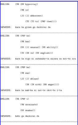
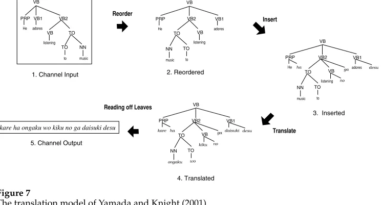
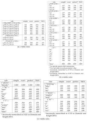
Figure 6 shows a portion of the bilingual English-tree/Japanese-string corpus used in Yamada and Knight (2001) and here. Figures 7 and 8 show the generative model and parameters; the parameter values shown were learned via specialized EM re-estimation formulae described in this article’s appendix. According to the model, an English tree becomes a Japanese string in four steps.

First, every node is re-ordered, that is, its children are permuted probabilistically. If there are three children, then there are six possible permutations whose probabilities add up to 1. The re-ordering depends only on the child label sequence, and not on any wider or deeper context. Note that the English trees in Figure 6 are already flattened in pre-processing because the model cannot perform complex re-orderings such as the one we described in Section 1, S(PRO,VP(V,NP))→V, PRO, NP.

Figure 6

Figure 7

The translation model of Yamada and Knight (2001).

Figure 8

The parameter tables of Yamada and Knight (2001).

Second, at every node, a decision is made about inserting a Japanese function word. This is a three-way decision at each node—insert to the left, insert to the right, or do not insert—and it depends on the labels of the node and its parent.

Third, English leaf words are translated probabilistically into Japanese, independent of context.

This model effectively provides a formula for P(Japanese string |English tree) in terms of individual parameters, and EM training seeks to maximize the product of these conditional probabilities across the whole tree/string corpus.

We now build a trainable xTs tree-to-string transducer that embodies the same P(Japanese string|English tree).

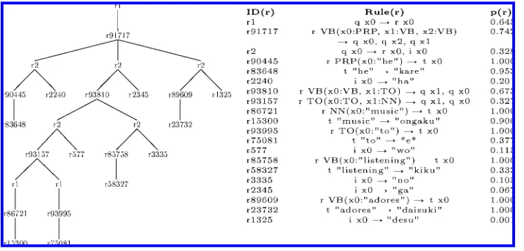
It is a four-state transducer. For the main state (and start state) q, meaning “translate this (sub)tree,” we have three rules:

q x0→i x0, r x0 q x0→r x0, i x0 q x0→r x0

State i means “produce a Japanese function word out of thin air.” We include an i rule for every Japanese word in the vocabulary:

i x0→“de” i x0→“kuruma” i x0→“wa” . . .

State r means “re-order my children and then recurse.” For internal nodes, we include a rule for every parent/child sequence and every permutation thereof:

r NN(x0:CD, x1:NN)→q x0, q x1 r NN(x0:CD, x1:NN)→q x1, q x0 . . .

Therhssends the child subtrees back to state q for recursive processing. However, for English leaf nodes, we instead transition to a different state t, so as to prohibit any subsequent Japanese function word insertion:

r NN(x0:“car”)→t x0 r CC(x0:“and”)→t x0 . . .

State t means “translate this word,” and we have a rule for every pair of co-occurring English and Japanese words:

t “car”→“kuruma” t “car”→“wa” t “car”→*e* . . .

This follows Yamada and Knight (2001) in also allowing English words to disappear (therhsof the last rule is an empty string).

Every rule in the xTs transducer has an associated weight and corresponds to exactly one of the model parameters.