Recursive analysis and estimation for the discrete Boolean random set model

Rochester Institute of Technology

RIT Scholar Works

Theses Thesis/Dissertation Collections

3-1-1996

Recursive analysis and estimation for the discrete

Boolean random set model

John Handley

Follow this and additional works at:http://scholarworks.rit.edu/theses

This Dissertation is brought to you for free and open access by the Thesis/Dissertation Collections at RIT Scholar Works. It has been accepted for inclusion in Theses by an authorized administrator of RIT Scholar Works. For more information, please [email protected]. Recommended Citation

Recursive analysis and estimation for the discrete Boolean

random set model

by

John C. Handley

B.S., The Ohio State University (1978) M.S., The Ohio State University (1981)

Submitted to the College of Science

in partial fulfillment of the requirements for the degree of

Doctor of Philosophy

at the

ROCHESTER INSTITUTE OF TECHNOLOGY

March 1996

©

Signature of Author.

Center for Imaging Science May 14, 1996

Center for Imaging Science Rochester Institute of Technology

Rochester, New York

Ph.D. THESIS

CERTIFICATE OF APPROVAL

The Ph.D. Degree Thesis of John C. Handley has been examined and approved by the thesis

committee as satisfactory for the degree requirement of Ph.D. in Imaging Science

Approved by .

Edward R. Dougherty, Ph.D. - Thesis Supervisor Professor, RIT

Approved by .

Peter G. Anderson, Ph.D. - Committee Member Professor, RIT

Approved by .

Ronald Jodoin, Ph.D. Committee Member Professor, RIT

Approved by .

Francis Sand, Ph.D. Committee Member Professor, Fairleigh Dickenson University

Center for Imaging Science Rochester Institute of Technology

Rochester, New York

Ph.D. THESIS RELEASE PERMISSION

Title of Thesis: Recursive analysis and estimation for the discrete Boolean

random set model

I, John C. Handley, hereby grant permission to the Wallace Memorial Library of

the Rochester Institute of Technology to reproduce my thesis in whole or in part. Any

reproduction will not be for commercial use or profit.

John C. Handley

Recursive analysis and estimation for the discrete Boolean random set

model

by

John C. _Handley

Submitted tothe Center for_ImagingScience

on22 March _1996, inpartial fulfillment ofthe

requirementsfor thedegreeof

Doctorof_Philosophy

Abstract

Randomsetsprovide a powerfulclass of modelsfor images containing randomly placed objects

ofrandomshapesandorientation. Thosepixels withintheforegroundare membersofa random

set realization. The discrete Boolean model is the simplest general random set model in which

a Bernoulli point process (called a germ _process) is coupled with an independent shape or

grain process. A typical realization consists of_{many overlapping} shapes. Estimation in these

models_{is difficult owing}to thefactthat_manyoutcomes oftheprocess obscure other outcomes.

The directional one-dimensional _{(ID) model, in} which random-_{length line segments emanate} tothe rightfrom germs onthe_line,is analyzed viarecursive expressions to provide a complete characterization ofthesediscretemodels in termsofthedistributionsof their black and white

runlengths. An analytic representationis given for the optimal windowed filter for the

signal-union-noise_process,wherebothsignaland noise areBooleanmodels. Severaloftheseresults are

extendedto thenondirectional case where segments can emanateto theleft and right. Sufficient

conditions are presented for a two-dimensional _(2D) discrete Boolean model to induce a one dimensional Booleanmodel on an _intersectingline. When inducement _holds, the likelihood of

runlength observations of the two-dimensional model is used to provide maximum-likelihood

estimation of parameters of the 2D model. The ID directional discrete Boolean model is

equivalentto thediscrete-timeinfinite-serverqueue. Analysis fortheBooleanmodelisextended

Contents

1 Introduction 1

1.1 Background 4

1.1.1 Firstcontactdistribution 7

1.1.2 Steiner formula ₈

1.2 Organization 8

2 Analysis ofthe ID Boolean model 10

2.1 Fundamental events 13

2.2 Maximum-likelihoodestimation ₁₈

2.3 Runlength analysis ₂₃

2.4 Optimal filter ₂₈

3 Two-dimensional estimation with linear samples 42

3.1 _Motivating example ₄₃

3.2 Inducement ₄₆

3.3 Union ofBooleanmodels ₅₅

3.4 Maximum-likelihoodestimationfor random rectangles . . 56

3.4.1 _{Vacancy 58}

3.4.2 Likelihoodfunction forrandom rectangles ₅₉

3.4.3 Unionof rectangle processes ₆₁

3.5 Estimation for theunion ofBooleanmodels ₆₂

3.5.1 Randomtriangle process ₆₂

3.6 Tonerparticle example 65

4 Estimationwith multi-dimensional linear samples 69

4.1 Cross-windowed likelihood function 71

4.2 Estimation forrandom-rectangle model 74

4.3 The Boolean randomfunction 79

4.4 PyramidBooleanrandom function 85

5 _Queueing interpretationofthe ID Boolean model 90

5.1 _Busytimedensities 91

5.2 Depletion time 92

5.3 _Busy time fora specified number of arrivals 96

5.4 Number ofcustomers 100

5.5 Nonhomogeneous arrival and serviceprocesses 103

5.6 Occupation time 105

5.7 Service times_dependingon order of arrival 106

5.8 Batch arrivals 109

5.9 Optimal estimator 112

6 Analysis ofthe nondirectional ID Boolean model 114

6.1 Themodel 115

6.2 Fundamentalnondirectional events 116

6.3 Likelihood function 123

6.4 Optimalfilter forthe signal-union-noise model 125

7 Conclusion 133

8 _Bibliography 134

9 Appendix 140

9.1 Fundamental events and probabilities 140

List

Figures

2-1 Example_covering 12

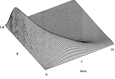
2-2 Likelihood function forobservation _(1,5,1) fora uniform segment length density.

p=_0.19, 0=5. Max _prob. = 0.016 ₂₀

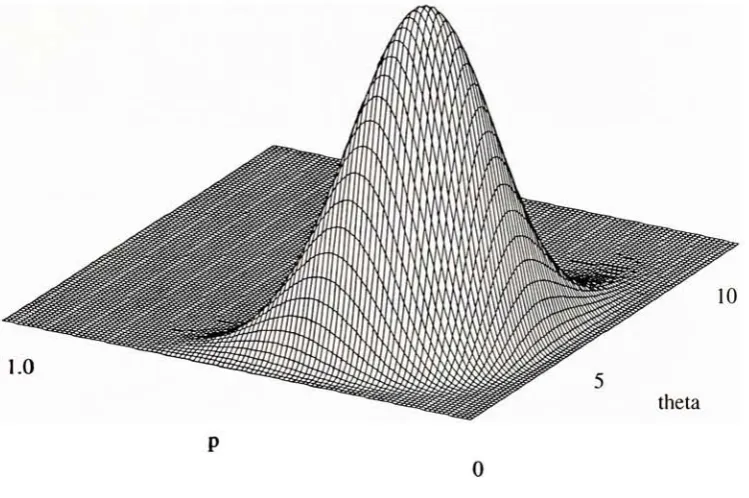
2-3 Likelihood function _assuming the segment lengths are_{Poisson distributed, p} =

0.69, 6=_{0.12. Max prob}= 0.015 21

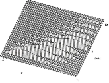
2-4 Likelihood function for observation _{(0,4,2,2,2,6,9,7,0)} for a uniform segment

length _{density, p}=_0.21, 0=6 ₂₃

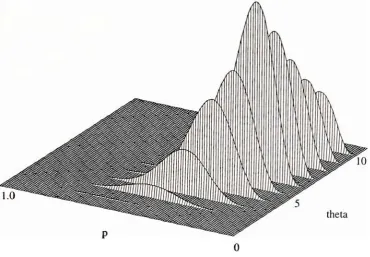
2-5 Likelihood function for observation _{(0,4,2, 2, 2, 6, 9, 7,0) assuming} the segment

lengths arePoisson distributed, p=_0.23, 9=_{2.4 24}

2-6 Samplerealizations for_p=_{0.3 and} 9=

0.0,0.5,...,4.0 25

2-7 Samplerealizations for 6=_{2 and}

p=_0.1,...,0.9 25

2-8 _E(l,m;fc) 33

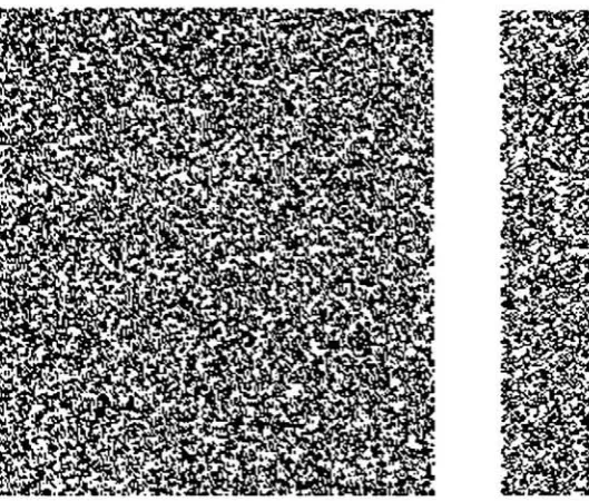
3-1 Realizations of model 1 _(left) and model2 _(right) 44

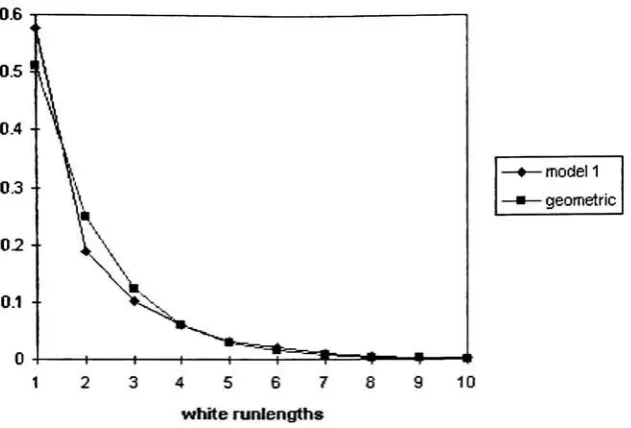
3-2 Whiterunlength and geometric densitiesfor model 1 45

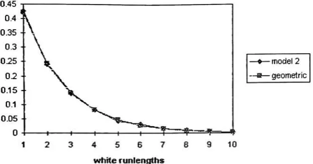
3-3 White runlengthand geometricdensities for model 2 46

3-4 Diagram ofestimation viainducement . 47

3-5 _{Events contributing}to Booleanmodel onthe line 57

3-6 Realization of 2D Boolean model of rectangles with independent widths and

heightswith meanlengths3and_6,respectively. _{Intensityis p}=0.1 _and

vacancy

is 16.5 60

3-7 A righttriangle induces a segmentlength ₆₂

3-9 _Horizontallyand _verticallyconvex connectedcomponents found in toner micro

graph 65

3-10 Actual _(left) versus simulated _(right) toner image 68

4-1 Cross sample of ablack blob (left, right, up, down) =

(K^,K^,Ky,Ky) 72

4-2 Realizationof a random rectangleprocess 75

4-3 Estimated bias for_{p, themarking probability}estimator 75

4-4 Estimated biasfor_0, themean rectangle width estimator 76

4-5 Estimatedbias for_{/x, the} meanrectangle height estimator 76 4-6 Estimatedcoefficient ofvariation for_p,estimate ofthe _marking probability. ... 77 4-7 Estimated coefficientof variation for_9, themean width estimator. . '. 78 4-8 Estimated coefficientofvariationfor_/x,themean height estimator 78

4-9 Resultsof_fittinga random-rectangleBooleanmodelto thegravel image. See text. 80 4-10 Cross-windowedobservation withgray-levelinformation 83

4-11 Samplerandom-pyramidimageswith_pincreasingclockwisefrom p= 0.04 in_the

upperleft-handcornerto0.08 88

5-1 Busy-time densitiesfor shifted-Poissonservice times with mean 6 93

5-2 Depletion-timedensities forshifted-Poisson servicetimes with mean6 95

5-3 Densitiesfor Nwhen theservice-time_densityisshifted Poisson with mean 6. . . 102 5-4 Densities for N given _H() when the service-time densities are shifted Poisson

withmean 6 . 103

5-5 _{Nonstationary}busy-time probabilities 104

5-6 Occupation-time densities for shifted-Poissonservicetimes withmean 6 106 5-7 Busy-time densitieswhen service-timesdependon order ofarrival 109

5-8 Busy-time densitiesforbatch arrivals 110

5-9 Densitiesofthenumberofcustomersinthesystemwithbatcharrivals atapoint

in time giventhat thesystem is _busy 113

6-1 Event _W(l,2) 116

6-2 Event _{2>4}(1,6) 118

List

Tables

2.1 Statistics for_0; 1000 trials; 9=2 ₁₉

2.2 Statistics for_p; 1000_{trials; p}=_{0.3 22}

2.3 Statistics for 6 as_{p varies;} 0=2 ₂₂

2.4 Statistics for_p as_pvaries; 0=2 ₂₂

2.5 Statistics for 0 as 0_varies;p=0.3 ₂₂

2.6 Statistics for_p as 0_varies;p=0.3

. 22

2.7 Optimal filter for Example 15 40

2.8 Optimal filter forExample 16 41

3.1 Statistics ofMLE from 50 realizations of the rectangle process for a range of

markingprobabilities. 0=_3,

p=6 ₆₁

3.2 StatisticsofMLEfrom50realizations ofunion ofrectangle andtriangle processes. 65

4.1 Estimatedbias 89

4.2 Estimated cv ₈₉

5.1 Probabilities xlO3

of a_busyperiod oflengthm and n arrivals ₉₉ 5.2 Conditionalprobabilities xlO3

of n customersserved given _busy period lengthm.100

6.1 Sixoutcomes_comprisingevent _E[!

2](1,2) 118

Chapter

1

Introduction

Binaryimages can be modeled as sets where objects in a image are considered sets of pixels.

These models are attractive inthat _they arise from first principles: random shapes placed at

random positions. The Boolean model plays an important role in the _theory of random sets

because it represents the simplest general such process. The one-dimensional _(ID) case has

applicationsinsignal_processingand_queueingsystems _{[5], [51],} [52]. Thetwo-dimensional _(2D)

model is used in geostatistics and image _{processing, among} other applications [3], [31], [39],

[40]. ThecontinuousBooleanmodelconsistsoftwo_{independent processes,}a shape process and

aPoisson point process. The outcomes ofthe shape process aretranslated to outcomes ofthe

point process. A typical realization consists of_{many overlapping}shapes.

Ourconcerniswith theID and2D discrete cases and our results will_ultimatelybe applied

to _{processing images.} Ourlanguage willreflect our application so that points are synonymous

withpixels,pointsina random set realization are called blackwhilepoints notintherealization

are called white. In the ID case, realizations will be _alternating sequences ofblack and white

pixels, thelengthsofwhichare called black and white runlengths.

A discrete random set is a measurable _mapping from an abstract _probability space to

subsets of the digital plane. Put _simply, a discrete random set is a collection of point sets

and theirprobabilities. It is convenient to model arandom set as two independent processes:

a shape process and a point process. The shape process is a particular type of random set

whoseoutcomes areboundedsubsets. Inimage processing, theshape process modelsobjectsof

ofthegrain process arecalled grains or primitives. The point processisused tomodel random

placement oftheshapes. Thepointprocess isalsocalled agerm process and the outcomes are called germs. ABernoulliprocessisapoint processinwhichthenumber of points marked in a

boundedsubset ofthedigitalplaneisarandomvariable_havingabinomial density. Therandom

variables_{corresponding}todisjointsubsets areindependent. Theprobabilitypof asingle point being markediscalled the _{marking probability} or rate. The outcome ofa Bernoulli process is

a set of pointseach selectedwith _probabilityp. A discrete Boolean model is a discrete grain

process _alongwith aBernoulligerm process.

Leta grain processS haveoutcomes_{si,S2,. .

}andlettheoutcomesofthegermprocessbe

{ii2,- --}- Oftenit isconvenienttoincludethenullevent0as apossible outcomeforadiscrete

grain sothat the class of grain realizations istaken to be _{0,s\,S2,- - .}. With this convention,

we omit the germ process notation and view theBoolean model realization as _arising from a

sequence of_trials, one at each point in the digital plane. The event 0 denotes the event that

no shape _occurs, that is the point is unmarked, and has probability _F(0) =

q = _{I p. This}

allows us to denote the entire model as alist of shapes _(including the null _shape) and their probabilities.

We make adistinctionbetweenthe discrete_{Boolean model,} whoseoutcomes arecollections

of sets and theobserved random set whichisthe union of outcomes oftheBoolean model. For

us, theoutcomeofthe Booleanmodelisthecollection _{s\+i,2+2, } What is observed, however, is the set _Uj(si + &)- The random set formed _{by taking} the union ofthe outcomes

of the Boolean model is called the germ-grain model. This distinction is made because we will compute probabilities of observations viatheBooleanmodel. Since _many events from the Boolean model can producethe same_observation, we need language to discriminate between

thefundamentaland simplereventsoftheBooleanmodel and the observed process.

Estimation in the continuous _theory is guided _by formulas _{linking probability} statements

aboutthegerm-grain process with_probabilitystatements_regardingthegerm and grain process

separately. Germ-grain realizations are what are_observed, someasurements ofthe germ-grain observations can be _directly related to the germ and grain processes. Statements about the

grain process involve Minkowski functionals ofthe _shapes, often in terms of mean area and

quite generaleven without _introducing randomness. Most applications assume shapes regular enough sothat theserandom variables are_easilyparameterized.

Insteadof_drawinguponthecontinuous_theory,our approach is to attack the discrete case

directly. We first show that the ID Boolean model and thegerm-grain process are equivalent

formulationsofthesamerandom process. _{In particular,} the distributionofthe Boolean model is completelydetermined_bythegerm-grain process. Theconsequence ofthis result isthat the IDBooleanmodelisobservable: theBooleanmodelisdetermined_{byits sampling distribution.} Moreover,given_anydistribution forthesegment lengthsoftheBoolean _model, it is a straigh-forward matter to write downthe _{governing distributions} of the germ-grain process. This is in contrast to the continuous case where the _{relationship is in} terms of an integral equation involvingthe Laplace transformofthe segment length distribution (Hall [23], page 102).

Therecursiveformulasand eventstructuresneededtoshowthisequivalence are generalized

to computethe optimalfilter or point estimatorfor one Boolean model unioned with another.

Specifically, given a windowedobservation ofthe union oftwo Boolean models (or germ-grain

models), what is the best estimate ofwhether a point is covered _by one process but not the

other. Atypicalscenario iswhen one Boolean model represents signal and the other noise. If apixelis black inthe union,whatisthebestguessas towhether it is reallywhiteandcovered bynoise?

Theseresults are quitegeneral and go beyondimage processing applications. One dimen

sionalBoolean models also model _queueing systems where a line represents discrete time and

a point is marked if a particle enters the system at that time. The segment length is the timeinterval (or service _time) that the particle occupies the system. Multiple arrivals cause

overlapping occupancy times. A reasonable question is what is the service time distribution given the busy-time distribution? Or conversely, given the service time _{distribution,} what is

thebusy-time distribution? Thesequestions are answered _bythe result _linking the germ-grain

model _{(busy times)} and the Boolean model (for service times). If two types of particles can

enterthe_system, what isthebest estimatethat one type ofparticle is in the system and the otheris not, giventhatwe observethe_occupancyofthesystemforawhile? This is answered_by

the optimal filter. Densities ofseveral other random variables ofinterest are given in Chapter

Once the ID problem is _{solved, the} solution is leveraged to estimate parameters of 2D

processes. A fullrecursivesolutionin the2D_settingappearsbeyondreachdue tocombinatorial

explosion, but progress is made _{by looking} at the ID processes produced by 2D processes intersecting with fines. _{Likelihood functions for 2D} models are expressed via horizontal and

vertical _{runlengths, assuming}independence ofthe perpendicular processes. While practical in many instances, this methodcan be improved _bycomputingthejoint distributions ofvertical andhorizontal blackand white_runlengths, respectively. The joint distribution is computed_by

analyzing how 2D grains intersecta "'cross.'"

Theoriginalformulation requiresthe segments toemanate froman _endpoint, which serves

as the "center'1 of the grain. This restriction can be relaxed to provide a description of the germ-grain model given _{any Boolean} model formulation where the centers of the grains are

within thegrain.

1.1 Background

Inthis section,wereviewthebasicpropertiesofBooleanmodelsandshowhow_theyare usedfor

estimation. The Booleanmodel is a random closed set which is composed of two independent

random processes: a germ process and a _primarygrain. The germ process is a Poisson point

process while the _primary grain is a random closed set. Often the _primary grain is required tobe convex. Throughoutthis work wedeal _exclusivelywith_stationary processes. Let _{&};<=/ be a realization ofthegerm process and let _{5j}ie/ be realizations ofthe grain process. The

germ-grain model realization is S = _Uie/(&+Si), the random set that isobserved. The most

important property ofBooleanmodels isdue to Matheron [35]: for _anycompact set _K,

P(SnK^) =

l-exp{-\E

||Sb

if||}

where5b isthe_primarygrain, K denotesthe reflection ofK about _{the origin,} E is expectation

and A is the _intensity ofthe Poisson process. The quantity on the left is called _{the capacity} functional or _hitting distribution. This fundamental equation relates thegerm-grain model to

thegerm and grain processes. The_capacity functional completely_describes

A fundamental quantity ofthe Boolean model is the volume fraction or mean fraction of

the area covered by 5, per unit area: _p= _{P(0 S). Intuitively,} this _{quantity describes how}

densethe realizationsaie on average. The complement 1 _p ofthe volume fraction is called

theporosity. A consistent estimator ofthe volume fraction is simply the ratio of covered area

to sampled area in arealization.

Sometimesit ispossibletomakeuseofhigherorder statisticsforestimation. Thecovariance

of pores is definedtobe

CP(z) =aw(0i S,zi S) =exp{-AE||(z+_S0)USb||} - (1 ~

pf (1-2)

It turns out that forthecaseof aBooleanmodelwhere the_primarygrain is a diskof random

radius, the covariance of pores and the _{porosity completely determine} the _intensity of the

Poisson process and the radius distribution of the _disks, and vice-versa. This relationship

follows from explicit formulas _{linking (Cp,p)} and _(A,F), where F is the radius distribution

(Hall _[23], pp. 299-300). Onecould_conceivably estimate Cp and_p from data and solve for A

andF. _But, the_{relationship involves}anintegralequation andisthusnot suitedforestimation.

Aconsistent estimatorfor Cp is

1 Cp(z) =

\\l(ui,Vj both white) n .

=i

1 n

^2

(1.3)

for a sample of points_"Ui,Vi, i =

1,. . .

,n and z =

Ui V{. Note that z is a vector and that a

realization should be sampled in many directions and distances. _Consistency is with respect

to n > oo withthe samples _rangingover an unbounded subset of the plane. This estimator

was used _by Diggle [9] (see also Hall_[23]) to fit a random disk model to ecological data not

resembling disks in any way. _However, the method is of interest because it demonstrates a common estimation technique. The covariance function was estimated _{from a realization and}

fitted in the least-squares sense, with a theoretical covariance function where the disk radius

had a three-parameter distribution. Thus minimization was carried out over four variables

(includingA). Whilethefittedmodelbearsnoresemblanceto theoriginal_data,suchatechnique

might be usefulfor discrimination among Booleanprocesses.

in Dupac [18]. Inthis method, thediskradii are assumedto benormally distributed: N(p,a2)

with 3a _{> p,} sothat the_probabilityof a negativeradius issmall. _Using Eq. 1.1,

l-p=exp{-A(/>2

+<72)}. (1-4)

The method proceeds _{by sampling} circular _clumps, i.e. those connected components in a

realization which aredisks. Circular clumps could have been formed _by isolated _disks, disks

fallingcompletely insideotherdisksordisks_coveringotherdisks butnothitting_anyother. The

radiiofcircularclumps areobservable, buttheradii oftheconstituentdiskscannotbeobserved. By computing the probabilitythat a circular_clump occurs given that adisk ofa given radius

occurs, one can use Bayes' theorem to compute the radius density of circular clumps. This density is approximately normal whose mean and variance are functions of_p and a and can

be estimatedfrom a realization. Then _{A, p} and a1

can besolved for in termsofthe estimated mean,estimated_variance, and estimated porosity. The resulting threeequationsarenonlinear.

Thismethoddemonstratesa method of moments approach. _Namely,iftheoreticalvaluesfor

parametersof an observable process are related_functionallyto theparameters ofthe_underlying

Boolean _model, one can replace the theoretical parameter values of the observed process _by

estimates and solveforthe parameters inthe _underlying process. One must be careful in this approach to not have an underdetermined systemof equations. The system of equations _are, as inthis _case, often nonlinear. _Also, the statisticalproperties ofsuch estimates are unknown

ingeneral and often must be determined viacomputer simulations. On the other _hand, these

estimatorsare often the_only ones availablefor random sets.

Ayala et al. _[1] went beyond Dupac and sought to investigate the statistical properties

ofthis method. _They made several _{modifications,} however. _First, there is no advantage to

assumingnormaldistributed diskradiisincethe_densityof circular_clumpradii canbecomputed numerically whatever the disk radius distribution. Ayala et al. chose to model the radius

distribution as uniform on [0,p]. This has the advantages of _being nonnegative and _having

intensity A and radiusparameter_pcould be formed:

(A,p) =

argmaxTT/(r;;\p).

x,P XA

1.1.1 First contact distribution

Thefirstcontactdistributionis animportanttoolfortheanalysis of a random set and Boolean

modelsin particular. It isdefined to bethe_{probabilitythat,} giventhat a point is not covered bytherandom set,ahomotheticofsome_structuringelement Bintersects the random set: for

r _>0,

HB(r) = l-P(SnrB^$)/(l-p). (1.5)

Thechoice ofBgivesdifferent probesintotherandom set and elicitsdifferentproperties. This

issimilar inspirit togranulometries. Fora2D Boolean model withconvex _primary grain and

convex set _B,

Hs(r) = ₁

-exp

^E

(2,]rkE[Wk(So)}W2.k(B)

whereu>2 =ttisthevolumeofatwo-dimensionalunit_sphere,and_WkareMinkowskifunctionals:

W0(K)= _\\K\\

, the area ofK

Wi(K)

-\\dK\\/2, one-halftheperimeter ofK (1.7)

W2(*0=_ca

usingthese _definitions, equation 1.6 can besimplified to

HB(r) =1

-exp

j-A

]^E

||fl||]

}

The structuringelementis_typicallyaline or aball.

Ayala et at _[2] use thederivative ofEq. 1.8 to form a maximum likelihood estimate of a

Boolean model. The first contact distribution is observable from the germ-grain model. For

a _realization, a _{(widely scattered)} sample of points are taken and of those not _{covered, the} distance to the closest covered point is measured (assuming B is a ball). The approximate

et aL do this for therandom disk model and provide simulation results for the coefficient of

variation ofthe estimator forvarious values ofPoisson_intensity and mean radius.

1.1.2 Steiner formula

Oneofthemostuseful expressions_relatingtheBooleanmodelandthe germ-grain modelis the

generalized Steiner formula [53]. It generalizes the expression Eq. 1.1. For So convex and K

compact and _convex,

XE\s0k = Y^{2}\E[W2(SQ))W2-k(K) (1.9)

where the Minkowski functionals in thesummand are defined in Eq. 1.7. Note the _similarity

with Eq. 1.6. The quantityon the _{left is tp(K)} = ln(P(KC S)) and can beestimated from

realizations:

(se_k) nw

*>

|snH,, (1.W)

for convex, compact _structuringelementsKand observation windowW. In the case of regular

geometric_figures, the_primarygrain canbeparameterized andthe Minkowski functionals (and

theirexpected_values) obtained. TheRHS ofEq. 1.6 isthen expressedin terms ofdistribution

parameters andMinkowskifunctionals ofthe_structuringelement K. _By suitablechoices of K

and scalings olK (linesand_{disks,typically),}one can obtain randomfunctionsonthe left tobe

fittedwith parameterizedfunctionsontheright. Theparameters_providingthe best fit serve as

estimatesoftheBooleanprocess parameters. CressieandLaslett [8] use a least-squares _fitting

approach _along with scalings of disks to estimate a Boolean model with _randomly oriented

quadrangle _primary grain. Such techniques depend on the grain _having tractable Minkowski

functionals and expectations. As inthe other cases, the statistical properties of the estimates

are determined throughcomputer simulations.

1.2 Organization

This thesis is organized as follows. Chapter2 contains results specific to the basic _{ID model,}

process. The firstpartreviewsthefundamentalevents _{pertaining to the}Booleanmodel onthe line. Amoredetailedexpositionisfound in_Doughertyand_Handley [12],which establishes the foundation uponwhichthisentire thesisrests. Nextwe lookat how these fundamental events

are usedtodomaximum-likelihoodestimationforthe_markingprobabilityand parameters ofthe segment length distribution. The likelihood function can reformulated in terms ofrunlengths instead ofBoolean model events. It is first shown that the distributions of black and white

runlengths can beexpressed intermsofthesegment lengthdistribution ofthe Boolean model

andvice versa. Thesequence ofblackandwhite runlengths are showntobeindependentrandom

variables. Thesetworesults establish_explicitlytheequivalencebetween ID germ-grainmodels andtheirBooleanmodels. Fromrunlength_{distributions,}wecan expressthelikelihoodfunction of a Boolean model observation as a function of the segment length distribution _parameters,

average whiterunlength andhistogramoftheblackrunlengths inthesample. Anoptimal filter forthe union oftwoBoolean models (one _signal, one _noise) given a windowed observation of

theunion processisexpressed astheconditional expectation ofthe signal at a point given the lengthand position oftheblackunion runlength withinthewindow. Suchafilter iswell-known

tobeoptimal intheminimum mean-absolute-error sense. To derivesuch aresult requiresthat

the fundamental events be generalized to account for all the events where the noise covers a

point but thesignaldoesnot.

Chapter 3 coverstheproblem ofinducementofID models onlines _intersecting2D models.

Estimation using linearsamplesisexploredforseveralsynthetic modelsas well as anapplication

involving tonerparticles.

In Chapter_4,weextendthenotion oflinearsamplestomulti-dimensionalorcross-_windowed

samples. These statistics provide better estimators than the linear samples as our examples show. We also _apply the _sampling procedure to the Boolean random function model and we

supplysimulationstoexploreitsperformance.

Chapter 5 returnsto the ID Boolean model and applies recursive event decomposition to

analyzingthediscrete infinite-server queue. _Manydensities ofinterest _{in queueing theory} are givenas recursive expressions. Numericalexamples followeach derivation.

Finally, in Chapter 6 we generalize_many ofthe results of Chapter 2 and _[12] to the case

Chapter

2

Analysis

the

ID

Boolean

Inone_dimension, shapes arelinesegments_havingrandom lengths. Forthepurposes of model ing, one must choosetheposition ofthe ''center"

of a segment length. _Here, we choose the left end-point so that thesegments are said to emanate to theright on the line. Thegrain process S has integer-interval outcomes _[0,k _1] of length _k, where k is a random variable _taking

positive values. If_{p denotes} the_{marking probability} and_C(k), k =

1,2,. . . thesegment length distribution, then the_probabilityof alinesegment oflength lessthan or equalto _{k emanating}

from a point is q +_{pC(k), q} = 1 p. _{This probability} captures both the _probability that a

segment doesnot appearandthe_probabilitythat if it does appear, its lengthis no longerthan

k. _{Alternatively,} in the ID _{case, the} Boolean model is _fully described _by a sequence ofi.i.d.

random variables _representing segmentlengthswith distribution

F(k)=

q +pC(k), k=_{0, 1,}. . . (2.1)

(where_C(0)= 0). Ateachpointionthe_line,Xi =0 if_thepoint is _{notmarked. If}

A", =k _{> 0,}

then thelinesegment [0,A; _1] isplaced theresothat theoutcome is [i,k+ i l\. This_{way, the}

marking probability p= 1 _F(0) isfoldedintothesegment length distribution

providing more

elegant expressions. Points onthe linewill beeither covered or left uncovered _by the process. Anobservation consists of_alternatingsequences of covered and not-covered points.

A Booleanmodelis arandom set_consistingoftwoindependent processes: a point process

processwhere points on the discrete fineare marked with _probabilityp. The shape process is

a linesegment of randomlength_startingat theorigin.

The pointprocess isalso calledthegermprocess and outcome are called germs. Theshape

process iscalledthe grainprocess whose outcomes are called grains. AnoutcomeofaBoolean

model is a collection of sets. If _{;i E _1} are thepoints marked _by the Bernoulli process and

{[0,Xj l];i G _/} are the random-length line segments, then the outcome is the collection of

intervals _{[fi,Xj+_& l];i G /}. _{Corresponding} to the Boolean model is a germ-grain model (germs aremarked points andgrainsare sets). Thegerm-grainmodel is formed _{by taking}the

union ofthesets output fromthe Booleanmodel: _Uig/[j,:rj +_& 1]. Thusthe outcome ofa

Boolean model is acollection of setswhile theoutcome ofits germ-grainmodel is a set. The

indicator functionofthegerm-grain modelis a_binaryrandom process that is observed. Since a segment at the origin is completely determined _by its _length, the shape process

can beidentifiedwith a random variable_takingpositive values. _Moreover, whether a segment

appears atapointor notisgoverned_bya_binaryrandom variable. Thesegment lengthrandom variableandthegermrandom variablescanbecombinedforma single sequenceofi.i.d. random variablestodescribethe entire process: a onedimensional discrete Booleanmodel is identified

with asequence ofindependent_identically distributeddiscreterandom variables _A", > 0 where theevent (Xi =₀₎ means that the point i is not marked andthe event _(Xi =

k) where k > 0

meansthat theset [i,i+k _1] isa member oftheoutcomeoftheBooleanmodel, i.e., the point

i is marked andthe linesegment [0,A: _1] is movedto i. Let F denote the distribution of_Xi

sothat the entire Booleanmodelisspecified _{by F. In particular,} the _{marking probability is p}

= _1-F(0).

Theoutcome (Xi =_k) is_saidtocoverapoint_jifk >0 andi <_j < k. Apoint i iscovered

ifsome outcome _{among {(Xj} =

hf) :_{j <i}} covers i. It isoften convenient to speak of point i

covering point _{j by}which wemeanthe outcome of arandom variable at i covering j. Figure

2-1 depictspoint 1 covering_itself, and points 4and 5covering 7.

ABoolean modelwillbe denoted_byXandits corresponding _binaryrandom process_byYx

ifwe need to_specifywhichBoolean model or _simplybyY if its correspondingBoolean model

is clear from the context. The event _(Y(i) =

xi x._A x

Figure 2-1: Example covering.

binaryrandom variable_Y(i)isafunctionof{.. .

,Xi-i,X{} andcertainlytheY(i)'s are highly

dependent as asingle segment length can cover _many points. In Fig. 2-1 the segment length

random variable outcomes are _{X\ = _{1, X2} = _{0, A3} = _{0, X4} = _{5, X5} =

4, Xq = _{0, X7} = _0,

Xg =

0) while the _{corresponding binary} random process outcome is (1,0,0,_1,1,1,1,1). The

lengthof a contiguoussequence ofpoints wherethe_binaryrandom process is 0is called a white

runlength while thelength a contiguoussequence of l's iscalled a black runlength.

We will show that for the one-dimensional discrete _{case, the} Boolean model and Y are

equivalentinthesensethatF completely determines Y andfromthejoint_density ofYwe can

computeF. _Moreover, the _density ofY is expressible interms of the densities ofthe lengths

of contiguous sequences of covered and uncovered points (black and white _runlengths, respec

tively). This allows us to do what we call runlength analysis ofBoolean models. _Indeed, Y

isan _alternatingsequence {.. .

,u)j,(3j,Vj+ii0j+i,. .

.} ofdiscretepositive independent random

variableswhere_Ujcorrespondstowhiterunlengths and_(3j toblackrunlengths. _Expressingthe joint _density of a windowed observation ofY in terms ofF is the major result of_Dougherty

[12] but nowwegofurther anddescribetheentire process in terms of F. Theconverse means

thateven though thesegments ofX overlap and obscureeach other _{causing many} events ofX

to yieldthe same event of_Y, the length distribution F is _fully determined _by the runlength

densitiesofY.

Firstwe will review severalfundamentalevents ofXandtheir probabilities. We thenshow

how these are related to the indicator function Y and establish that X and Y are equivalent.

runlengths.

2.1 Fundamental events

Consider an interval of points 1 torn. Events will be discussed for this particular interval

simplytomakenotation convenient. _Owingto_stationarityoftheBoolean model (the random

variables_Xi are_i.i.d.),probabilities oftheseeventsdependonthelengthoftheintervalbutnot

on the position. Events will be denoted _by reference to particular points. In [12], the events

were denoted _by thelength ofthe interval onwhich _they occurred rather than the particular

interval. We need to adopt a more explicit notation here in order to compute the optimal

filter. Ifthe event notation here were altered to reflect _only the interval _length, all notation

wouldreduce to thatfoundin [12]. Oftentheevents will appear inrecursive expressions,so we

establish the _followingconventions. Let _A(i,j) denote some unspecified event on the interval

[i,j]. If i =_j, denote_theevent

by A(i) andif_j <_i,denotetheevent _byA(0). Note that_A(0)

maynot represent _anyactual_event, butoften serves as a placeholder to start a recursion.

Let_{E'(l,m) be}theeventthatpoint miswhite, i.e.,none of_X\,. . .

,Xm coverm. (E (i) is

theeventthat idoesnot cover_{itself, namely (Xi}=

0) andfor technical reasonstobe apparent

later wedefine E ₍₀₎astheentire event space). Thisevent_{is easily}seentobe decomposed into

independent events:

E'(l,m) = (Ii<m-l)nE'(2,m).

(2.2)

Byinduction and_{independence,}

m

P(E'(l,m)) =HF(i-l).

(2.3)

i=l

Let _E(l,m) be the event that segments _emanating from points in the interval cover the

interval and no segment extends beyond. That is, (X\,...,Xm) is exactly self-covering. Note

that, since the segment length random variables are independent at each _{point, E(l,m) does}

occur arelisted below:

X\ X2 A3

1 1 2 2 1 2 2 0 1 2 2 0 0 1 1 1 2 2 2 2 3 3 3 3 3 3

The_followingproposition showshow an E-even

(2.4)

can be_recursively decomposedinto inde

pendent, disjointevents_{enabling its probability}to becomputed.

Proposition 1 _E(l,m) has decomposition

m k

E(l,m) =

1J U

l,m)] k=lj=l

(2.5)

where the union is disjoint and has probability

i-i

F(E(l,m)) =

(F(m)

-1))

J]

-l)P(E(j + _{l,m)) (2.6)}

t=i

urtere_P(E(0)) = ₁

and_P(E(i)) =

F(l) - F(0).

Proof. This proof_{is substantially different} from the one in _[12] and is more consistent with

the event structure used in this work. In this proof we make explicit how to decompose _any

Let u) G RHS ofEq. 2.5. Then _X\ = k for _some 1 < k < m, i.e. X\ covers _[1,/c] and [k+_1,m] iscovered _{by E(j}+_1,m),j < /-. _Therefore, a;G_E(l,m).

Conversely,let u;GE(l,m). Then_X\ =kforsome 1 < k< m since 1 must cover itselfbut

cannot extendbeyond to _bydefinition. Let

j=_{max{1,max{Z : [2,}

1] doesnot coverI and I < _{m}} (2.7)}

Itmust be that_j <fcelse_jisuncovered in _[1,m] and u _E(l,m). We distinguish two cases. First,if j =_1,thenno pointintheinterval beyond 1 isuncovered. That_is,u> E _E(2,m). Inthis

case u) G_E'(2,1) =

E'(0) =

theentireeventspace. _Therefore,u E _(Xx =

k) fl_E'(0)n_E(2,m),

as required. If_j > _1, then _j is not covered _{by any} points in _{[2, j]} so that to E (2,_{j) by} definition. Nowa*

G_Efj

4-1,m) forifthereissomepoint I not covered _by [j+_1,/] thenone of

twocontradictions willbereached. IfI< _k,thenI is not covered_{by [2, /]} since_j is not covered

by [2,j]. But thisimplies that_j was notthe largest index in Eq. 2.7. If / > _fc, then I is not

coveredbyT nor_{by [2TZ],} henceit isnotcoveredat all intheinterval. _Therefore,

uE(X1 = k)n_E'(2,

j)n_E(j+_{1,m) (2.8)}

forsome_{j in} [1,fc]. Aswas_shown, itmust bethat_j <k < m. When_j= k=mthe firstpoint

covers theentireinterval but [2, j] doesnot cover m. In_{this case,}

u> g_(X1 =

to)nE(2,m)nE(m +1,m) = (Xi =

m)D_E'(2,m) nE(0). _(2.9)

which motivatesthedefinitionof_E(0) asthe entire event space and _P(E(0)) =_1. As for _{disjointedness,}consider

S = (Xi = _fc)nE,(2,j)n

Efj"

+_l,m)n_(Xx = _{k')nE'(2,/) nE(f+1,m).}

(2.10)

It must be that k = _{if, else}E = 0. Without loss of_generality, let _j < j' and suppose there

Theevents(Xi = _{fc),E'(2,.7'), and}

E(j+l,m) are allindependentsince_theyare outcomes of

disjointcollections ofindependent random variables _{X\}, {X2,. ,Xj}, and {Xj+\,... ,Xm},

respectively (except inthe case wheretheE'-eventorE-event is the entire spacein which case

the disjoint collectionsare _{Xi} and {X2,.. .

,Xm}, respectively).

The probabilityexpression inEq. 2.6 follows _{bydisjointedness,} independence andEq. 2.3:

F(E(1,m)) =

EfcLi E?=i P_[(Xi =

fc)n_E'(2,j)n_E(j+_1,m)], by disjointedness =

EtLi E*=iP&i =_{k)P(E'(2,j))P(E(j+l,m)), by}independence

= E

1E2L;^P(Xi =k)P(E'(2,j))P(E(j+l,m)), by reordering =

Y?=ilF(rn)

-F(j

-1)]Y\>r\Hi ~

l)P(E(j+_Lm)), using Eq. 2.3.

How is a point i not covered? _First, it cannot cover itself: _Xi = 0. Second,

any segment

emanatingfrompointsto theleftmustbetooshorttocoverit. Ifwedenote by W(z) theevent

that a point i isnot _covered, it is theevent

TV

W(z)= lim _C](Xi^<j) N>oo ! '

j=0

and has probability

N N

F(W(t))=

P(W(0))= lim

I]

J]

In _[12] it is shownthat the limit exists for _probabilitydistributions with finite means defined

onnonnegative integers.

Related to _E(l,m) are the events _D(l,m) and G(l,m). The event _D(l,m) is the event

thatthem points cover themselvesbut thesegmentlengths emanatingfromwithin_mayextend

beyondthelastpoint. For_example,a sample member ofD(l,2,3)is (Xi =_5)n(A"2 =

3)n(A~3 =

0). Note that _{D(l,m) depends only} on outcomes ofthe random variables X\,...,Xm. It is

shown in [12] that D(l,m) has _probability

m j1

P(D(1,m))= ₁

-F(m)+

YsiFim)

F(j

-1))

J]

-l)P(D(j +_{1,m)) (2.12)}

where _P(D(0)) = 1 and _P(D(i)) = 1

-F(0) since _D(i) = (Xi _> 0). Equation 2.12 has a

simpler form asseem_by the_followingmanipulation. Let _dk = P(D(1 +_i,k + i)).

dm =₁

-F(m)+_TT=i(F(m) -F(j

-1))UUF(i

-l)dm_j

= 1~

F(m)+_{F(m) xUtl}F(i- l)^-

-=1F(j

-1)Flti F(i

-l)dm^

Now,

E=inti F(i

-Vdm-j =

E^iP(E'(2, j))P(D(j+1,to)), by definition

=

P{U2E'(2,i)nD(i +_l,m)

UD(2,m)}

=P(all_{events on [2,} m])

=₁

since_anyevent on _[2,to] iseitherin D_(2,to) orcanbe decomposed into E'

(2,j)C\D(j+_l,m)

for some _j = _{2,.--,to, wherej} is _{the right-most point not covered} (if _{any). Equation 2.12}

takes theform

m j ₁

PCD(l,TO)) =_{l-^F(j-l))I]^-l)^(D(j +}

l,m)) (2.13)

J=l i=l

The importofthisrepresentationisthat_P(D(1,m)) dependson _F(0),. . .

,F(m 1) and F(0),

. . .

,F(m 1) canbecomputedfromd\,. . . ,dm.

G(l,to) istheevent that the to pointsintheinterval _[1,m] are covered _bysegments ema

natingfrompoints within andtotheleftofthem_{points, but}not_extendingbeyondtheinterval.

That_{is, G(l,m)} Cf\<m(Xi < m i +₁₎ and_everypoint in _[1,m] is covered_bysome random

variableinthe_{coimtably infinite}collection {.. -_,X_i,A"o,X\,...

,Xm}. Provided that F isnot

"heavy-tailed"

(see _[12] for definition and_discussion) the event _G(l,m) has _probability

P(G(l,m+₁₎₎ =P(G(2,to +

1))- P(W(l))P(E(2,m

+ _{1)) (2.14)}

wherethe recursionis initiated by P(G(0)) = P(W(z))/F(0).

Let _H(1,to) denote the event that _[l,m] is covered, whether _{by internally} or _externally

segmentsextendfrompointstotheleftoftheintervaltocover pointsto theright oftheinterval. For example, (A"o =_to+

1) C H(l,m). It isshownin _[12] that

P(H(1,m+ _l)) =

P(H(1,to))

-P(D(1,m))P(W(0)) (2.15)

where_P(H(1)) = ₁-P(W(0)). Theevent_H(l,m) iscalled totalcoverage ofthe interval [l,m] [52].

2.2 Maximum-likelihood estimation

Wefirstconsidertheestimationproblem whenthesegmentlength distribution isparameretized. Given windowed observations C =

c, we would like to estimate _{the underlying} parameters of theBooleanprocess. Inparticular,we wouldliketoestimate the_intensitypandthe parameter 0ofthe segment_density (0 _maybea_{vector) byfinding}thevaluesthat maximizethelikelihood

function; inour_{case, it is}the_{density P(C)} fromTheorem 1of_[12] evaluated attheobservation c (see Theorem 40 in the Appendix). In _keeping with the usual notation for the likelihood

function, we will henceforth denote the window _density as _P(C;p,9) to emphasize that the density is a function of several variables when the parameters are unknown. The maximum likelihoodestimator is

(p,9) =

argmaxP(c;p,0) _(2.16)

Thegeneralproperties ofthemaximum-likelihoodestimator_(mle) areunknowninthiscasedue

to thecomplexityand recursive natureofP(C). Weare_particularlyinterested in unbiasedness and thevariance oftheestimator. The properties cannot be_{determined analytically}and must beelicitedthroughsimulations and numerical evaluations. Givenanobservationand parameter

values, the likelihood function is evaluated by simply implementing the recursive formulas in Theorem 40in theAppendix.

For demonstration purposes, we use two models for the segment lengths. The first model

i windowsize 8 16 32 64 128

mean

variance

coefficient of variation

6.60 57.60 1.15 3.31 22.3 1.46 2.21 3.48 0.84 2.08 0.89 0.45 2.00 0.30 0.27

Table2.1: Statistics for _0; 1000 _trials; 0=2

Poisson_density; that _is,

P(H=h)=_e-9h-1/(h

-1)!, h=l,... _(2.17)

The mean length in this case is 0

-1-1. This case will be referred to as _simply the Poisson

model, keeping in mind that the expected segment length is one more than the parameter

value. Figures 2-2 and 2-3 show _{likelihood functions for} the uniform and Poisson models of

the observation _(1,5,1), respectively. Both show the trade-off _{between p} and 9 in _trying to "explain"

asingle black run-length. Theoutcome could be the result of a sequence of_highly

probable short segments orthe resultofrarer but longersegments.

A more realistic example is given in Figures 2-4 and 2-5. _Here, with a window size of 32

observing (0,4,2,2,2,6,9,7,0) from thePoisson model with 0 = _{2 and}

p =

0.3, the likelihood functions show more definitive peaks. In both _cases, maximum-likelihood estimation yields

similarestimatesfrom a single _{observation, E(H)} =3.5 and_p= 0.21 in_{the uniform case and}

E(H) =3.4_and

p=0.23 in thePoissoncase.

How does the window size affect the estimation? From a practical statistical point of

view, thewindowmust be large enough tocapture several black to white and white to black

transitions: all white _(Z/m,oo) or allblack_(Hm) observations _carrylittle information. _Indeed, it

canbe easilyseenfromtheexpressionfor_(Lm,oo)intheAppendixand2.15that_p=0_maximizes

P(Lm,oo) to 1 and _p = 1 _maximizes

P(Hm)to _1, regardless ofthe length _{distribution,} {Ck}.

Estimationresultsforvarious window sizes areshown inTables 2.1 and 2.2 for a process with

segmentlengths_usingthePoissonmodel. Asthewindowsize_increases, thevariancesdecrease

and the averages approachthe truevalue. In Table 2.1 the coefficient of variation for 9 with

a window size of8issmaller than thevariance for awindow size of16. _{This is because} when

thewindow size is small, thereis agreater likelihood of_observing allblack or all white pixels

Figure 2-2: Likelihood function for observation _(1,5,1) for a uniform segment length density.

p=0.19, 0 =5. Max prob. = 0.016

or _1, respectively, and thevalue of0is irrelevant.

Togainfurther insight intothebehaviorofthe_MLE,we lookatthestatistics ofan example

wheretheparameters 0and_pvary. _Intuitively, iftheprocess resultsin outcomesthat are "too

white" or "too

black,"

one expects the estimates to be biased or have high variance because

there will be fewer black and white runs observed. The outcomes were generated _according

to aPoisson model with 0 = 2. A window size of32 was used again to observe the process.

Figures2-6and2-7showsamplerealizationsastheparametersvary. In Fig. _2-6,theparameter

0varies from 0 to4.0 while_premains fixed at0.3andinFig. _2-7, theparameter_p varies from

Figure 2-3: Likelihoodfunction_assumingthesegmentlengthsarePoissondistributed, _p= _0.69, 0= 0.12. Maxprob=_0.015.

For values of_p= 0.1 _through

p=

0.9,MLE 9and_p where obtained from 100 observations

ofthePoissonmodel_using a windowsize of32. Theresults are summarized in Tables 2.3and

2.4. _{Alternatively,}when_premainsfixed at 0.3and thevalue of0 _varies, the statistics ofthe

estimates are summarized in Tables2.5 and2.6.

Inall casesit isclearthatiftheobservations areeithertoowhite ortooblack dueeitherto

a small windoworextremeparametervalues inthe_{process, the maximum-likelihood estimates} will have highvariancesor bias.

The previous analysis required that the segment length _{distribution be parameterized in}

window size 8 16 32 64 128

mean

variance

coefficientofvariation 0.45 0.08 0.61 0.37 0.06 0.63 0.33 0.02 0.46 0.31 0.01 0.33 0.31 0.004 0.21

Table 2.2: Statistics forp; 1000 trials;p=_0.3

p 0.1 0.2 0.3 0.4 0.5 0.6 0.7 0.8 0.9

mean

variance

coefficient of variation

3.10 13.92 1.20 2.10 1.54 0.59 2.08 1.62 0.61 2.16 5.44 1.08 3.60 28.56 1.48 4.53 40.18 1.40 7.48 56.88 1.01 10.89 53.46 0.67 12.82 39.49 0.50

Table 2.3: Statistics for 0 as_{p varies;} 0= 2.

p 0.1 0.2 0.3 0.4 0.5 0.6 0.7 0.8 0.9

mean

variance

coeffient of variation

0.11 0.01 0.73 0.22 0.01 0.50 0.31 0.02 0.45 0.46 0.046 0.47 0.59 0.06 0.41 0.67 0.05 0.35 0.73 0.03 0.24 0.79 0.02 0.17 0.79 0.01 0.13

Table 2.4: Statistics forpas_pvaries; 9=_2.

9 0.0 0.5 1.0 1.5 2.0 2.5 3.0 3.5 4.0

mean

variance

coefficient of variation

0.10 0.03 1.70 0.52 0.13 0.71 1.05 0.67 0.78 1.69 2.17 0.87 2.24 5.61 1.06 2.83 4.15 0.72 3.10 7.92 0.91 3.33 10.50 0.97 4.51 21.64 1.03

Table 2.5: Statistics for 0as 0_{varies; p}=0.3.

0 0.0 0.5 1.0 1.5 2.0 2.5 3.0 3.5 4.0

mean

variance

coefficient of variation

0.29 0.01 0.26 0.31 0.01 0.31 0.31 0.01 0.39 0.32 0.02 0.44 0.32 0.02 0.42 0.34 0.04 0.56 0.35 0.04 0.54 0.41 0.04 0.51 0.45 0.06 0.54

Figure 2-4: Likelihood function for observation _{(0,4,2,2,2,6,9,7,0)} for a uniform segment length density, p=_{0.21, 0} =6

sincethere is a one-to-one correspondence between thesegment length distribution ofthe ID Booleanmodel and therunlength distributionsofits germ-grain model.

2.3 Runlength analysis

To describe theevent of a blackrun _havinglength _m, we must condition the black runlength

event on the event that a runlength _actually occurs. For _(Xq,. . .

,Xm+1) to produce a black

runlength of length _{to, it} must commence with a _W(0) event followed _by an _E(l,m) event

and tenninated _by a (ATm+i =

Figure 2-5: Likelihood function for observation _{(0,4,2,2,2,6,9,7,0) assuming} the segment

lengths arePoisson distributed, p=_0.23, 0= 2.4.

dependson all eventsto theleft (providedthesegmentlength distribution has infinite_support),

but the length ofthe blackrunlength,once_{it occurs, is} independent ofall events to the left of

the runlength. A black runlength _starting at 1 is precipitated _by a white to black _transition,

i.e. a point not covered point followed by a covered _point, which is the intersection of two

independent events: _W(0)DD(l). These twoevents are independent because _W(0) depends

on {Xj}j<o and_D(l) depends_onlyon {Xi}, twoindependent collectionsofrandom variables.

Theprobabilityofsuch aneventis P(W(0))P(D(1)).Theeventofmblackpoints preceded_by

awhite point andfollowedbyawhitepointisW(0)nE(l,m)nW(m + l). _However, thelatter

twoevents are not independentas _E(l,m) depends on {A"i,. . .

Figure 2-6: Samplerealizationsfor_p=0.3 _and9=_{0.0, 0.5,} ...,4.0.

Figure 2-7: Samplerealizations for 0=_{2 and}

p=

0.1,...,0.9.

on {Xi}i<m+i which contains {Xi,...,Xm}. The probability of the event can be computed

conditionally:

P(W(0)nE(l,m)nW(m +_l)) =P(W(0))P(W(TO +_{l)|W(0)nE(l,m))P(E(l,m)).}

(2.18)

The middle _{quantity is} the_probability that awhite point follows an E(l,m)-event. Since no

segmentlengthextendsbeyond _to,thismustbethe_probabilityof nosegment_{length appearing}

at m+_1, namely P(0). We can now write down the _{probability that} a runlength _{has length}

factthat _E(l,m) C_D(l),wehave for m= _{1, 2,}. . .

,

P(K=

to) =_{P(W(0) nE(l,m)nW(m +}

1)| W(0)DD(1))

=_P(w(0)nE(i,

m)nw(m+₁₎n_d(i))/p(w(o)n_d(i))

=P(W(0))P(E(l,m))P(W(m+l)|E(l,m))/[P(W(0))(l

-F(0))]

=_{P(E(l,m))F(0)/(l-F(0))}

Notethat P(K=

to) is just P(E(l,m)) scaled _byF(0)/(1

-F(0)) and soEq. (2.6) holds for P(K=

to) with therecursioninitiated_byP(K=

0) =F(0)/(1- F(0)).

Theeventthata white runlengthhas lengthmistheeventthata sequence of m white points ispreceded_byablackpointandsucceeded_byablackpointgiventhata black-to-whitetransition

has occurred. On the interval [0,m+_1] the _conditioningeventis _G(0) DW(l). These events

are not independent as _G(0) depends on the random variables {Xi}i<o and _W(l) depends the collection {X,-},<i. _However, the _probability can be computed conditionally: _P(G(0) fl

W(l)) = P(G(0))P(W(1)|G(0)). The latter probability is _{the probability,} given the point

0 is covered and no segment extends beyond _0, that 1 is white. Since 0 is _{covered, the only}

way for 1 not to be covered is for no segment to emanate from 1 and this _{has probability} F(0). The event that the points _[l,m] are white preceded and followed _by black points is G(0) fl_W(l) n. .. nW(m)nD(m + 1). The last event is independent from the others but therest all depend on {Xi}i<o. Once again we computetheprobabilities _using a _conditioning argument. Theoccurrenceof a white point at icauses all coverageevents at i + 1 andbeyond to be independent ofevents at i and beforesince if is _white, no segment at i or before can

reachi + 1 orbeyond. _Now,

P(W(i +_i)|W(i)n.. . nw(*)) =P(w( +i)|W()) (2.20)

isthe_probabilitythat apoint iswhitegiven that the pointbefore _{it is white,} which _{is simply}

ofwhite runs. Forto=_1,2,...

,

p(v=

m) =_P(G(0)n

n^i w(i)nD(m+ _i)|G(0)n_w(i)) =

P(G(0)P(W(1)|G(0))

xIIS1-P(W(i+ l)|W(i))P(D(m + 1))/ [P(G(0))P(W(1)|G(0))] (2.21)

=P(G(0))F(0)m(l

-F(0))/P(G(0))F(0)

= (l-F(0))F(0)m-1.

ThusV hasageometric_density with 1 _F(0) as_probabilityof "success."

Thelengthsofadjacentblackand white runlengths areindependent. First consider ablack

runlength oflength to followed _by a white runlength oflength n. As _before, an initial black

runlength_startingat 1 isinitiated_byawhitetoblacktransition: _W(0)PlD(l). Ontheinterval [0,1,. . .

,m4-n

4-1],theeventofaninitialwhite _point,followed _bymblack _points, followed_by n whitepoints_terminatingwithablackpointis_{W(0)DE(1,to)nf]"=m+i}W(t)nD(m+n + l). Thelasteventintheintersection is independentoftheothersbut therest aredependent. _Using

a _conditioningargument as_before,

P(K=_myV=

n) =P(W(o)nE(i,TO)nnr=r+iw(OnD(TO+n+ _{i)|W(o)nD(i))}

=

P(C&iW(i)|W(0)n_{E(l,m))P(W(0)}n_E(l,m)) xP(D(m+n+_{1))/[P(W(0))P(D(1))]}

= _p(E(i,m))p(n-r+i1

w(* + !)lw( + ₁₎n_W(0)n_E(l,to)) xP(W(m+_1)|W(0)n_E(l,to))

=P(E(1,to))P(W(to₊

1)|W(0) nE(l,m))

xnss+i'pcwci+ijiww)

=P(E(l,m))F(0)m

=_P(E(1,

to)) [F(0)/(1

-F(0))]F(0)"l"1(l

-F(0))

=P(K=_m)P(V= _n).

(2.22)

Nowconsiderawhiterunlength oflengthtofollowed_by ablack runlength oflengthn. On the

interval _[0,to-f-_n

blackrunlengthends with a whitepoint.

P(V=_m,K= n) =

P(G(0)nfl_iW()nE(m + 1,m+ n)nW(ro +n+ 1)|G(0)DW(l))

=

P(G(0))P(W(1)|G(0)) UZYP(W(t + l)|W(i))P(E(m + 1,m_{+ n)|W(m))}

xP(W(m+n+ l)|E(m +_1,m_{+ n))/}[P(G(0))P(W(1)|G(0))]

= F(0)mP(E(m_+l,m + n))

=P(V=_m)P(K= _n).

By induction, one can show _P(Ki =

mi,V= _n,K2 =

TO2) = _P(.Ki = _mi)P(F = _n)P(K2 =

m.2), P(Vi = _ni,/ir=

m,V2 =

TI2) = _P(Vi =_n{)P(K =_m)P(V2 =

",2), and so on. _Any finite

sequence oflengthsofblack and white runs areindependentfor the Boolean model.

Equations_2.6,2.19and2.21showhowtheblackand white runlengthdistributionsaredeter

mined _bythe segmentlength distributionoftheBoolean model. _{Combining these expressions,}

thesegment length distributioncanbeexpressed interms ofthe runlength distributions:

P(K=

to) +_Y.7=iF(j~

1)nCi F(i

-1)P(K=

m-j)

2Z?=iY]iZlF(i-l)P(K=

m-j)

F(m) =

---/^rj=r;j-r//v:r/r;

where _F(0) = _{1 P(V} = _{1). The one-dimensional discrete Boolean model}

is completely

described _by the runlength distributions. In other _{words, the} Boolean model is equivalent

to a random process of_{alternating independent black} and white runlengths where the white

runlengths have a geometric distribution. _Here, the Boolean model is completely observable.

This allows one to estimate the _{marking probability} and segment length distributions from

therunlengths. Runlengthobservationscan beusedformaximum-likelihood estimation ofthe

parametersof adiscrete Booleanmodel (Chapter3 and [24]).

2.4 Optimal filter

Ourmaininterest inthischapteristherole oftheBooleanmodel relativetodesignoftheoptimal

nonlinear filter inthe signal-union-noise _{(signal-union-clutter)} model. To form _{the model,} we

assumetheexistenceoftworandomclosed setsSand_A/",thefirst_beingthe_primarysignalgrain

by S= _{UiSi+Xi and} N =

UjNj+ *,-, respectively, where Si is identicallydistributed with 5,

Nj is_identicallydistributed withM, and Xi and_yj are random points. The observed image is

SUN. To filterthenoise and restorethe_signal, wedesirea translation-invariant filter $ such

that 17(SU_N)provides abestestimate ofS. _{Specifically,}wedesire \I> to minimizetheexpected value ofthesymmetricdifference \I>(SUN)ASat an _{arbitrarypoint,} where [*(5U_{N)AS] (2)} defines a binary-valued random function at each point z. _{Owing to stationarity, translation}

invarianceimposesno constraint on_{optimization; however,}selectionof\P is _typicallyrestricted

to some _familyoffilters and constraints are placed upon randomness in the signal and noise processes. Analytic formulationofthe optimization problem has been addressed _successfully

forr-openingsandgranulometricbandpassfilterswhengrains areassumedtobeeitherdisjoint ortheirintersectionsare constrained _accordingtosomestatistical model [10], [11], [13], [28].

Ifwe now considerthediscrete Booleanmodel, thepointprocess is aBernoulli processand

the _primary grain is a discrete random set [20]. Ifwe again require the optimal filter to be translation _invariant, but now restrict _{it only} to be windowed with window _W, then at each point _2, ty(SU_N)(z) depends_only on thepoints in the translated window W + z. _Assuming

W_{finite, ^(SUN)(z)}=

\P(fi,2,

---,m),wherei,2,--

-,m arethe randombinaryvariables definingSUNatthepixelsin W +z and *f> is interpretedas a windowfunction. Filtererror is given_{by E[\S(z) *(i,2,}

---,Cm)|] and isminimized by letting \17 be the binary conditional

expectation:

*(&,&, ,)={

1 _ifP(S(2) =

016,6,...,^) < 1/2

fnn^ (2.24) 0 _ifP(S(z) =0|i,6,...,m)>l/2

Hence,theoptimalfilterisdefined_bya_look-uptable: observethe_binaryvalues ₁,2, ,min the translatedwindow anddefine _ty(Sl)N)(z)=

*(fi,2,---,m) according to the _inequality P(S"(.z) =

0|i,f2,---,m) < 1/2- The filter $ possesses minimum error over all possible

windowed operators. ^ is usually called the optimal _{nonincreasing}filter because there is no

constraint_requiring^tobe_{increasing (however,} $canbe_increasingifminimum errorhappens to result from an _increasing filter). Optimal _{nonincreasing} translation-_{invariant filters have}

beenemployedinbinarydigital image_{processing, in particular,} to _{digital document processing}

design has been _{realization-based, meaning} that image-noise models have been employed to

simulate realizations and optimal _(suboptimal) filtershave beenestimated viatherealizations.

Our intent here _{is very} different. Weshall _{theoretically} derive the optimal filter for the

one-dimensional discrete Boolean model when the _primary grain is directional. This means that

P(S(z) = _{0|i,f2,---,m) must be expressed analytically. To} do so we shall extend some

fundamental resultsderivedin _[12] formaximum-likelihood estimation in the one-dimensional

discreteBooleanmodel. Whereasithasprovendifficulttoobtain_verygeneral resultsinthe

two-dimensional Euclideanmodelforeither statisticalestimationor optimal _filtering, the recursive

approachintroduced in _[12] fortheone-dimensionaldiscrete model has proven useful for both

one-_{andtwo-dimensional}

process estimation_[12] and nowforanalyticderivationoftheoptimal

clutterfilter inone dimension.

Before _derivingthe optimal windowed _filter, we first discussthe unionof Boolean models.

If X denotesa _binarydiscrete Booleanmodel with segment length distribution F, let {X'; i =

1,...,JV} denote a set of independent processes with segment length distributions {Fl;i =

1,. ..,JV}. The union of Boolean models is obtained by defining the union at each point.

Consider without loss of _generality the point 0. Let _Xq =

ki, i = 1,...,N. The _segment

length of random variable _Xq ofthe union is defined _{by taking} the union of segment lengths

emanating from 0 so that _Xq = _maxjfcj. In particular,

(A^o <