Ion solvent interactions

W. E. Waghorne, B.Sc. (Hons.)

This thesis is presented in partial fulfilment of the requirements for the degree of Doctor of Philosophy in the Australian National University •

Fellow, during the period September 1969 to August 1972.

Research School of Chemistry, Australian National University,

Canberra, A.C.T.

October 1972

-I would like to express my sincere thanks to Dr A.J. Parker for his expert guidance and continued support throughout the course of this work.

I would also like to thank Drs B.G. Cox and J.H. Sharp for their great assistance in carrying out this work.

This work was carried out with the financial support of an Australian National University Post-Graduate award, over the period September 1969 to October 1972.

Chapter I

Chapter II

Chapter III

Table of Contents

A Comparison of Some Extrathermodynamic

Assumptions for the Determination of the Free Energy of Transfer of Individual Ions

Introduction Results

Solubilities Rate Constants

The Ferrocene System Discussion

Page

1

6 8 11

The Reference Electrolyte Assumption 14 The Large Anion - Large Molecule

Assumption 17

The Large Cation - Large Molecule

Assumption 19

The Negligible Liquid Junction

Potential Assumption 20

Comparison of Assumptions 25

Conclusions 28

Liquid Junction Potentials Between Electrolyte Solutions in Different Solvents

Introduction

Results and Discussion EJ S

'

The Role of Specific Salvation in the Salvation of Ions

Introduction Results

Silver Cell Measurements

Standard Potentials of Other Metal Ions

29 31 33 41 45

47

Chapter IV

Experimental

Appendix

Bibliography

Discussion Conclusion

A Study of Ionic Salvation in Mixed Solvents Introduction

Results

Free Energies of Transfer of Individual Ions

Salvation Numbers of Ions Discussion

Some Applications of Work from this Thesis

Solvents Electrolytes Non-El ectrolytes Amalgams

Techniques

Potentiometry

Voltammetry and Electrolysis Solubility Measurements

Silver Salts

Other Electrolytes Stability Constants Kinetics

Henry's Law Measurements Calorimetry

Proton Magnetic Resonance

Page

56 62

63

64 67 88

94

102 104 106 107

107 109

Table 1 2 3 4 5 6 7 8 9 1 2 3 4 1 2 3 4 1 2

List of Tables

Chapter I

Solvent Properties

Solubility Products

Association Constants in Non-Aqueous Solvents

Second Order Rate Constants of Nucleophilic Substitution Reactions

Cyclic Voltammetry of the Ferrocene System

Limiting Equivalent Conductances of Ions

Silver Cell Potentials, Variation with the Bridge Solvent

Silver Cell Potentials

Free Energies of Transfer of Silver Ions

Chapter II

Mutual Heats of Solution of Solvents

Free Energies of Transfer of Solvents

Silver Cell Potentials, Similar Salt Bridge Electrolytes

Silver Cell Potentials, Dissimilar Salt Bridge Electrolytes

Chapter III

Solvent Properties

Silver Cell Potentials

Standard Electrode Potentials of Redox Couples

Free Energies of Transfer of Individual Ions

Chapter IV

Free Energies of Transfer of Ions in Mixed Solvents

Table

1

Applications

A Comparison of Electrorefining Processes for Copper

Page

Figure 1 2 3 4 1 2 1 2 3 4 5 6 7 8

List of Figures

Chapter I

Cyclic Voltammograms of the Ferrocene Couple Second Order Substitution Reactions

The Ferrocene-Ferricinium System

A Comparison of Free Energies of Transfer of Silver Ions from the Various Assumptions

Chapter_ll_

The Variation of Liquid Junction Potential with Changes in the Enthalpy of Mixing of the

Cell Solvents

The Relationship Between Enthalpies and Free Energies of Mixing of Some Solvents

Chapter IV

The Free Energies of Transfer of Ions in Acetonitrile-Water Mixtures

Free Energies of Transfer of Some Cations in Acetonitrile-Propylene Carbonate Mixtures Free Energy cf Transfer of Silver Ions in Dimethylsulphoxide-Propylene Carbonate Mixtures

Free Energies of Transfer of Ions in Dimethyl-sulphoxide-Water Mixtures

Fractional Free Energies of Transfer of Silver, Cupric and Sodium Ions in Acetonitrile-Water Mixtures

Fractional Free Energies of Transfer of Silver and Cuprous Ions in Acetonitrile-Propylene Carbonate Mixtures

Fractional Free Energies of Transfer of Silver and Cupric Ions in Dimethylsulphoxide-Water Mixtures

Fractional Salvation Numbers of Silver, Cupric and Sodium Ions in Acetonitrile-Water Mixtures

Figure

9

10

1

2

3

4

Fractional Salvation Numbers of Silver and Cuprous Ions in Acetonitrile-Propylene Carbonate Mixtures

Fractional Salvation Numbers of Silver and Cupric Ions in Dimethylsulphoxide-Water Mixtures

Applications

Potentials of the Copper-Cuprous and Cuprous-Cupric Redox Couples in Acetonitrile-Water Mixtures

Equilibrium Constants of the Copper, Cupric, Cuprous Equilibrium in Acetonitrile-Water Mixtures

Flow Diagram for the Electrowinning of Copper from Cuprous Solutions

Flow Diagram for 'Powder Refining' of Copper from Cuprous Solut ions in Acetonitrile-Water Mixtures

Page

86

87

97

98

100

Summary

This work consi sted of investigations into two areas of the chemistry of ionic solutions.

The initial work invoived the comparison of four types of extrathermodynamic assumptions which have been proposed for the

estimation of the free energy of transfer of individual ions from one medium to another. It was found that the four types of assumption,

the reference electrolyte, large anion-large molecule, large cation~ large molecule, and negligible liquid junction potential assumptions, gave essentially the same values of the free energy of transfer of the silver ion from acetonitrile to fourteen other solvents.

With a view to investigate the validity of the negligible liquid junction potential assumption, the liquid junction potential of a

variety of cells was studied~ A good correlation was found between the liquid junction potential and the interaction energies of the solvents forming the boundary, and evidence for the theoretical, as

vell as practical validity of the negligible liquid

j

unction potential

assumption

was

found

The remaining work was an investigation into the importance of specific ion-solvent interactions, particularly complexing of cations by solve:it molecules, to the salvation energy of ions. It was found that free energies of transfer of cations, from water to a variety of solvents, and the variation of free energies of transfer of ions with changes in the composition of some binary solvent mixtures, could be adequately explained in terms of specific ion-solvent interactions. Tn view of the generality and magnitude of these effects it was suggested

that specific ion-solvent interactions should form a part of any general theory of ionic salvation.

CHAPTER

I

A Comparison of Some Extrathermodynamic Assumptions for the Determination of the Free Energy of Transfer

of Individual Ions

In

any component, i, is equal in all of the phases present. For example

the free energy of an electrolyte in a saturated solution in any medium

is equal to its free energy in the appropriate solid phase, and

correspondingly equal to its free energy in a saturated solution in any

other medium. However, the concentrations of saturated solutions in

different media may be very different and so the free energy per mole

of solute can vary widely between different media. To compare the free

energies of different species in solution a formal standard state must

be defined, and for this work the molar scale, with the standard state

of a 1 molar solution, corrected to infinite dilution (in any solvent)

has been selected. The standard free energy of a species i in a

solvent, S, can be compared to its standard free energy in a reference

solvent, R, by equation 1 where a. refers to the activity of a lM l

~Go(i)S = ~G0 (i)R - RT ln(ai)S

(~)R

solution of i in the appropriate medium.

(1)

The term

free energy of transfer of one mole of i [~G (i)] from one litre of tr

infinitely dilute solution in solvent R to one litre of infinitely

dilute solution in solvent S. Therefore we have

~Go(i)s

=

+

tr

and ~G (i)

₌

tr

For non-electrolytes and whole electrolytes 8.G can be determined tr

exactly from measurements of thermodynamic quantities such as solubility.

However, as Guggenheim (1929) points out thermodynamic measurements

cannot be carried out on individual ions, for example the solubility of

sodium ions in water is an idea with no physical significance, and so

it is impossible to measure unambiguously 8.G values of individual tr

ions. Despite this, it is reasonable to assume that 8.G values of tr

strong electrolytes in dilute solution are composed of 8.G values for tr

each of the individual ions involved, and that estimates of the

individual ion components would provide information (Popovych, 1970)

about the processes involved in ionic salvation.

A variety of extrathermodynamic assumptions for determining 8.G tr of individual ions have been proposed, and these have been the subject

of excellent reviews by Parker (1969), Popovych (1970) and Kolthoff

(1971).

The Born (1920) equation (4), where Z. is the ionic charge of i, l

(4)

e

0 the charge of an electron, ri the ionic radius of i and SR and s5 the dielectric constants of solvents Rand S respectively, provides the

basis of much of our understanding of ionic salvation, and so is the

basis of the assumptions proposed. From equation (4) it is apparent

that the smallest values of 8.G should be for large ions with single tr

charges, and should exist between solvents with equal or similar

dielectric constants. Also, since the ionic charge appears as a squared

term, 8.G should be equal for an anion and a cation of equal radius and tr

charges between any two media. A second source of salvation energy

which must be accounted for is specific solvent, solute interactions,

assumptions proposed either assume that this is negligible, particularly for large ions, or that it can be compensated for as a neutral component of salvation energy.

Pleskov (1947) proposed that the ionic salvation energy, and hence the redox potential of a sufficiently large cation would be constant and chose the rubidium ion (r = l.48A0 , Pauling, 1940) as a suitable reference.

Later Coetzee and Campion (1967) calculated a value of 6G (Rb) · tr

from water to acetonitrile, based on the Born equation (4) and a corrected ionic radius for the rubidium ion.

Feakins and Watson (1963) determined values of 6G (H+) and 6G

tr tr

(Cl) from water to water-methanol mixtures by plotting 6G of the tr

halogen acids and alkali metal chlorides against the inverse of the radius of the counter ion. The value of 6G for the individual ions

tr

were taken as the value of 6G at infinite counter ion radius (i.e., tr

-1

r =

0).

the appropriate inert gas, in their values of 6G . tr

A second approach to the problem is to equate the 6G of an ion tr

with that of either a second, oppositely charged ion or a neutral molecule.

The species chosen for this type of assumption are almost

invariably large complex ions with alkyl or aromatic ligands presenting an essentially non-interacting surface of hydrogen atoms to the

surrounding solvent. They are also chosen with similar sizes and ligands so that effects such as polarization and structure making or breaking should be similar. Strehlow (1952) suggested that 6G

tr

cobaltocene-cobalticinium systems were suitable for the assumption. The latter

system is unstable in many media but the former has gained considerabl e

acceptance, particularly among European workers (e.g., Breant,

et aZ.,

1970, and Barraque, Vedel and Tremillon, 1968). Grunwald, Baughman

and Kohnstam (1960) suggested that the assumption could be applied

to the large tetrahedral tetraphenylarsonium (Ph

4As+) ana

tetraphenyl-phosphorium (Ph

4P+) cations, tetraphenylmethane (Ph4C) and the

tetra-phenylborate (Ph

4B) anion. The combinations of these available

provide a group of easily compared assumptions. Of these the reference

electrolyte assumption involving Ph

4AsPh4B has gained the widest acceptance (cf. Kolthoff and Chantooni, 1971, Parker and Cox, 1972).

Popovych and Dill (1966) suggested that triisoamyl-n-butylammonium

tetraphenylborate (TABPh

4B) would be a suitable reference electrolyte. Parker and Alexander (1968) proposed two assumptions of this type

involving the transition state and reactant in carefully selected

organic substitution reactions. They also suggest that in certain

cases it may be possible to suppress the liquid junction potential in an electrochemical cell, by separating the half cells with a salt

bridge,. and to determine .6Gtr values from measurements of these cells.

Assumptions involving reference electrolytes -or reference ions

and non-electrolytes are the most popular of the assumptions proposed

and are experimentally the simplest to use. Therefore it seems likely

that any universally adopted assumption will be of this type. In view of this, and the fact that no assumption can ever be proved correct

or incorrect, it was decided to compare ~G values from a reference tr

solvent into a variety of other solvents based on some of these

assumptions.

Because of the large amount of available data, the silver ion

was chosen for study and values of ~G cj,_g,+) based on the different

tr-....

MeCNa a P.C. Me

2

a _{DMAa DMSOa HMPTa MeOHa}

EtOH HCONH

2a H Oa MeN0

2

..

Bp (0c) 80.1 100.8 241.7 56.2 285 152.5 202 165.5 189 235 " 65. 0 78.3 193 100.0 74

Mol. Wt. (M) 41 61 102 58 120 73.1 99.1 87.1 78 179 32 46 45 18 100 Density

g.ml- 1

(d20°C) 0.7856 1.1354 1.0257 0.784625b 1.2615300 0.9445 1.0327 0.9366 1.1014 1.0253 0.7914 0.78506250 1.139 0.9982 1.3816250 C Dielectric

constant

(E) (25°c) 37.5 38.6 _{64.4 21.26200 44300} 36.7 31.5 37.8 48.9 29.6 32.6 24.30 109.5 78.5 26.14c Dipole ~

Moment (D) 3.84 3.44 2.72 4.69 3.82 4.09 3.79 4.3 5.37 1.70 1.68 3.25 1.84

Viscosity _d

(25°C) cP 0.345 0.62 _{0. 295~·300} 9.87300 0 .. 796 1.83 0.919 2.000 0.345 0.547 1.08 3.31 1.00 1.780 Refractive

index n 20 1.3441 1.3935 1.4212 1.356092501.4742300 1.4269 1.4706 1.4351 1.4783 l.344l 1.3288 1,35941250 1.4453 1.333 1.768c

D

a) A.J~ Parker, Chem. Rev., 69, 1, (1969).

b) Electroanalytical Chemistry, Vol.,

2,

1969),

d) J. Murto and E.L. Heino, Suomen. Kem. B, 39, 263, (1966).

e) Abbreviations: MeCN, acetonitrile; MeN0

2, nitromethane; P.C., propylene-carbonate; Me2co, acetone; TMS, sulpholane; DMF,

dbnethylforroamide; NMePy, n-.methyl-2-pyrrolidone; DMA, dimethylacetamide; DMSO, dimethylsulphoxide; HMPT, hexamet

hyl-phosphoramide; "MeOH, methanol ; EtOH, ethanol; HCONH

2, form.amide; H2o, water; TFE, t r ifluoroethanol,

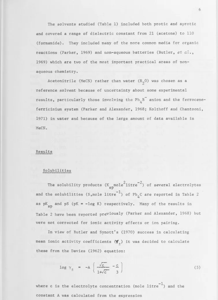
The solvents studied (Table 1) included both protic and aprotic

and covered a range of dielectric constant from 21 (acetone) to 110

(formamide). They included many of the more common media for organic

reactions (Parker, 1969) and non-aqueous batteries (Butler,

et

al.,

1969) which are two of the most important practical areas of

non-aqueous chemistry.

Acetonitrile (MeCN) rather than water (H

20) was chosen as a

reference solvent because of uncertainty about some experimental

results, particularly those involving the Ph

4B anion and the

ferrocene-ferricinium system (Parker and Alexander, 1968; Kolthoff and Chantooni,

1971) in water and because of the large amount of data available in

MeCN.

Results

Solubilities

The solubility products (K mole litre ) of several electrolytes 2 -2 sp

and the solubilities (S,mole litre ) of Ph-1

4

c

as pK and pS (pK = -log K) respectively. Many of the results in sp

Table 2 have been reported previously (Parker and Alexander, 1968) but

were not corrected for ionic activity effects or ion pairing.

In view of Butler and Synott's (1970) success in calculating

mean ionic activity coefficients ("f+) it was decided to calculate

these from the Davies (1962) equation:

log Y+

=

rc-1+/c

-

;

l

-1

where c is the electrolyte concentration (mole litre ) and the

constant A was calculated from the expression

Table 2

Solubility Products (K

sp

2 -2

- mole litre ) of solutes

K a -Log

- log S sp

Solvent f Ph Cc AgBr Agl AgN

3 AgSCN AgBPh4 Ph4AsBPh4 Ph4Asl 4

MeCN 1 ,,543 3.2 13.2b 14.5b 9.9b 10.3b 7.5b 5.8b 2.7b

1,479 3.4 21.9 22.7b b 18.lb 15.6 5.7 2.1

MeN0

2 17.6

P.C.

0..,686

Me

2

co

3.616

TMS 30° 1.244 2.7 18.7 19.0b 14.9b 10.2 5.2b 2.5

DMF 1 '9L1. _{) '} 2.5 15.3b 13.7b · 11. 3 b 11.8b 7.lb 3.9b 1.9b

N""MePy 2.004 2.0 14.2b 15.0 11.6 9.7b 4.9 3.3 2.1

D}fA

1.525

HMPT

2.036

XeOH 1.900 3.7 15.5b 18.6b 11.5b 14.2b 14.4e 9.0b 2.3b

EtOH 2.956 3.7 16.1 19.1 12.lb _{14.4 9.4 3.7}

HCONH

2 0.309 4.9 11.5b 14.6b ·8.0b 10.0b 10.3b 8.8b 2.0b H

20 0.509 7.8d 12.3b 16.0b 8.6b 12.7b 17.2e 17.3e 5.lb

TFE 2.657 19.7 23.4

a) This work unless otherwise indicated.

b) A.J. Parker and R. Alexander, J.

Arn.

c) - log solubility.

d) B.G. Cox, A.J. Parker, J.

Arn.

e) .M. Kolthoff and M.K. Chantooni, Anal. Chem., 44, 194 (1972; J.

Arn

.

Ch em . S o c • , 9 3 , 7 10 4 ( 19 7 1) •

f) Abbreviations as in Table 1.

g) Debye-Huckel A. parameters, l.823xl06 (sT)-312 using dielectric

A

=

(sT)3/2 (6)

wheres is the solvent dielectric constant and T the absolute

temperature. The A factor for each solvent is listed in Table 2 along

with the corrected solubility products.

The solubility products and ionic strengths in acetone (Me

2co), ethanol (Et0H) and trifluoroethanol (TFE) were also adjusted for ion

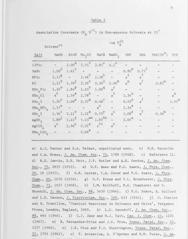
pair formation. Association constants for the tetraalkylammonium

salts and the iodides of various cations are similar in solvents of

similar dielectric constant (Table 3) so that the ionic strengths of

electrolytes were estimated from the strengths of related electrolytes.

The association constant of Ph

4Asl was taken to be 150 in acetone, in line with those of similar electrolytes, and that of AgClo

4 was taken

to be < 100 in all solvents other than Me

2co, which is consistant with

values in methanol (Me0H), Et0H, MeCN, and nitromethane (MeN0

2), all of which have low dielectric constants (Table 1).

No measurements involving the BPh

4 ion could be carried out in TFE because the ion was unstable in this acidic medium. Also AgPh

4B

was apparently too soluble (>0.SM) in hexamethylphosphoramide (HMPT)

for meaningful measurements to be made.

Rate constants

-1 -1

The second order rate constants (k, mole litre sec ) for the

aromatic substitution reaction (SNAr) of azide ion with

para-nitrofluorobenzene, and the substitution reaction (SN2) of thiocyanate

Table 3

Association Constants (KA M-1) in Non-aqueous Solvents at 25 0

l og Kdd

Solventcc A

Salt Me0H Et0H Me

2co MeCN MeN02 DMF DMA TMS(30°) TFE LiPic 2.ooa 2.91 b 2.82c 4.2c

NaBr 1.ood 1.61c 0.90e 0.75f

KPic l.llg 2.46b 2.18h s i s f

KI l.lld l.70j 2.26k 0.301 1.60m s n s f 0.81m

NEt

4Pic 1.26° 1.84P 1.65b 1.ooq

C s

NBulj_Cl s r l.59S 2.78k s t l.34u s a

NBu

4I l.20r 2.09S 2.37a 0.48v 0.92

2 f

1.95a s

NBu

4BPh4 1.57w

X

1.34a s

NEt

4I 1.36c 2.llS 2.lla 0.70y

C

1.082 f 0.56m

s s

AgN0

3 1. 89j -2. 41 j 5.43aa l.85bb 2.60n AgCl0

4

C

1.56c 2.26a bb C

s s s

NBu

4c104 2.06a

a) A.J. Parker and D.A. Palmer, unpublished work.

and C.A. Kraus, J. Am. Chern. Soc., 70, 1709 (1948).

b) M.R. Reynolds

c) Reference 12.

d) R.E. Jervis, D.R. Muir, J.P. Butler and A.R. Gordon, J. Am. Chern.

Soc. , 75, 2855 (1953). e) D.P. fuileS and P.G. Sears, J. Phys. Chern. ,

59, 16 (1955). f) G.R. Lester, T.A. Gover and P.G. Sears, J. Phys.

Chern. , 60, 1076 (1956). g) D.F. Evans and T.L. Broadwater, J. Phys.

Chern., 72, 1037 (1968). h) I.M. Kolthoff, M.K. Chantooni and

s.

Bhownik, J.

Arn.

and B. Trernillon, 'Chemical Reactions in Solvents and Melts', Pergamon

Press, London, England, 1969. k) L.G. Savedoff, J. Am. Chern. Soc.,

~ , 664 (1966) . 1) G.J. Janz and M.J. Tait, Can. J. Chern., 45, 1101

(1967). rn) R. Fernandez-Prinz and J.E. Prue, Trans. Farad. Soc., 62,

1257 (1966). n) J.E. Prue and P.J. Sherrington, Trans. Farad. Soc.,

57, 1795 (1961). o) F. Accascina, A. D'Aprano and R.M. Fuoss, J. Am.

Chern. Soc. , 81, 1058 (1959). p) R. Whorton and E.S. Amis, Z. Physik.

Chem. (Frankfurt), 17, 300 (1958). q) C.M. French and D.F. Muggleton,

J. Chem. Soc., 2131 (1957). r) R.L. Kay, C. Zawoyski and D.F. Evans,

Table 4

-1 -1

Second Order Rate Constants (k, mole litre sec ) of Nucleophilic

Substitution Reactions at 25°c

Solvent Reactants

-RX+ y

CH

3I + NEt4SCN

CH

3I + NEt4Br

4N0

2C6H4F +

NEt

4N3

b

MeCN

-1.82

-1M20

-3.3

log k C

P.C. Me

2co NMePy DMSO

-1.69 -0.82 -0.28 -1. 32

+1.0

-3.02 -2,3 1.9a -3.3

EtOH

-3.5a

a) This work; all other rate constants are from A.J. Parker,

Chern. Rev., 69, 1, (1969).

b) Abbreviations as in Table 1.

c) All reactants at 0.02 + 0.05M.

(Continued from p. 9)

TFE

-5e4a

J. Phys. Chern., 69, 4208 (1965).

Phys. Chern., 72, 3281 (1968).

s) D.F. Evans and P. Gardarn, J.

t) R.L. Kay, S.C. Blum and H.I.

Schiff, J. Phys. Chern., 67, 1223 (1963). u) H. Elias and H.

Strecker, Chern. Ber., 99, 1019 (1966). v) D.F. Evans, C. Zawoyski

and R.L. Kay, J. Phys. Chern., 69, 3878 (1965) ~ w) M.A. Coplan and

R.M. Fuess, J. Phys. Chern., 68, 1177 (1964). x) D.S. Berns and R.M.

Fuess, J. Am. Chern. Soc., 82, 5585 (1960). y) A.I. Popov and N.E.

Skelly, J. Am. Chem. Soc., 76, 5309, (1954). z) P.G. Sears, E.D.

Wilhoit and L.R. Dawson, J. Phys. Chern., 59, 373 (1955). aa) V.S.

Griffiths and K.S. Lawrence, J. Chern. Soc., 1208 (1955). bb) H.L.

Yeager and B. Kratochvil, J. Phys. Chern., 73, 1963 (1969).

The Ferrocene-Ferricinium System

+

The ferrocene-ferricinium (Fe - Fe) system was studied by cyclic voltammetric measurements on cell A.

Solvent S Solvent S

Ag

I

I I

I I

Fe (2xl0-4M) TEAP (0.02M)

I

where TEAP is tetraethylammonium perchlorate and the results are

listed in Table

5.

In

-5

saturated solutions of Fe (ca. 2xl0 M, Barraque, Vedel and Tremillon,

1968) were used.

Low electrolyte concentrations (0.02M) were used to minimize salt

activity effects and from the Henderson equation (D.A. Maclnnis, 1961, chap. 13; cf. Chap.

II)

in cell

A.

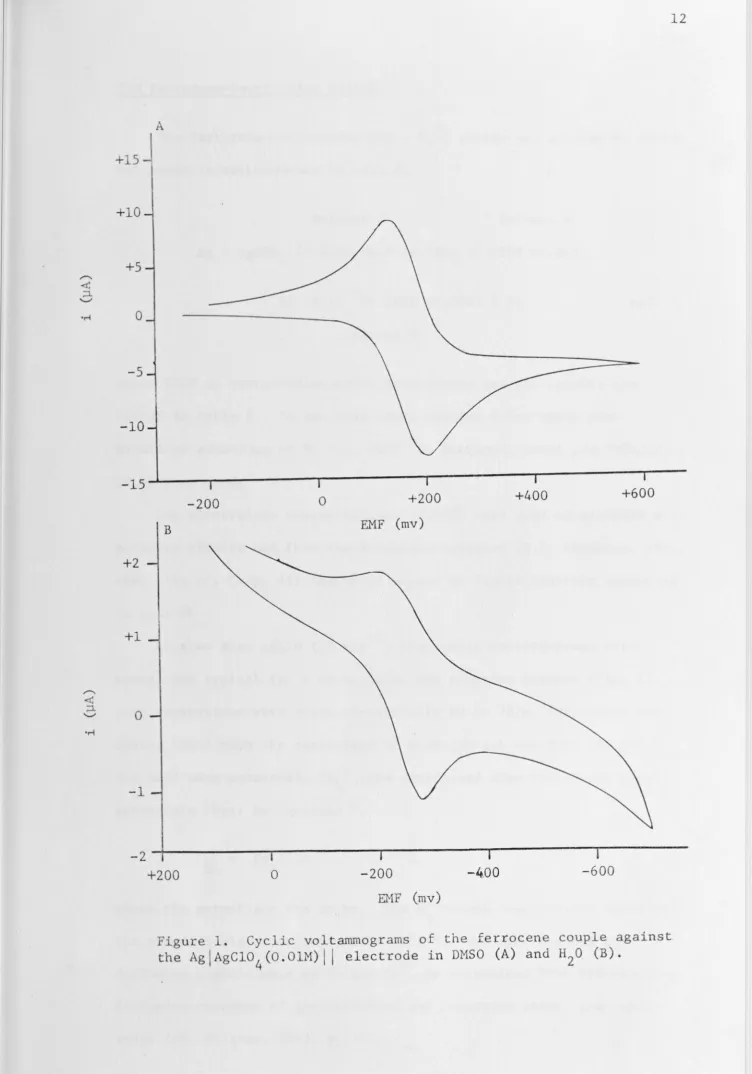
At slow scan ratio (lV min-1) the cyclic voltammograms were

normal and typical for a reversible, one electron process (Fig. l); peak separations were characteristically 60 to 70 mv (Nicholson and Shain, 1964) with the exceptions of Et0H (90 mv) and HMPT (80 mv). The half wave potentials (E_{1 )} were determined from the anodic peak

72

potentials (Epa) by equation 7.

= Ep -28

a (7)

where the potentials are in_mv. The E₁ values measured are close to

72

the standard electrode potentials (E0 ) for the system since the

+

diffusion coefficients of Fe and Fe , as determined from the relative

+10

+5

... 0

-5

-10

B

+2

+l

-1

-2 +200

-200 0

0

+200

EMF (rnv)

-200

EMF (rnv)

+400 +600

-400 -600

Figure 1. Cyclic voltammograrns of the ferrocene couple against the AgjAgCl0

The Ferrocene-Ferricinium System

+

The ferrocene-ferricinium (Fe - Fe) system was studi ed by cyclic

voltammetric measurements on cell A.

Solvent S Solvent S

Ag

I

I I

I

Fe (2xl0-4M) TEAP (0,02M)

I

Solvent S

where TEAP is tetraethylammonium perchlorate and the results are

listed in Table 5. In the case where solvent S was water near

-5

saturated solutions of Fe (ca. 2xl0 M, Barraque, Vedel and Tremillon, 1968) were used.

Low electrolyte concentrations (0.02M) were used to minimize salt

activity effects and from the Henderson equation (D.A. Maclnnis, 1961,

chap. 13; cf, Chap. II) one would expect no liquid junction potential

in cell ~

At slow scan ratio (lV min-1) the cyclic voltammograms were

normal and typical for a reversible, one electron process (Fig. 1);

peak separations were characteristically 60 to 70 mv (Nicholson and

Shain, 1964) with the exceptions of Et0H (90 mv) and HMPT (80 mv).

The half wave potentials (E_{1 )} were determined from the anodic peak Yz

potentials (Epa) by equation 7.

E₁ = Ep -28

Yi a (7)

where the potentials are in mv. The E₁ values measured are close to Yi

the standard electrode potentials (E0 ) for the system since the

+

diffusion coefficients of Fe and Fe , as determined from the relative

diffusion currents of the oxidation and reduction steps, are nearly

Ag

Table 5

Cyclic Voltammetry in the Cell

AgClo

4 (0.0lM)

TEAP (0.0lM)

Solvent

-MeCN C

MeN0 2 P.C. Me 2co C Sb

TMS 30°

DMFc NMePy DMA DMSOc HMPTc MeOHc Et0H HC0NH 2 H 20 TFE

TEAP ( 6. 62

1:)

+a E0,0lM Ag

mv

Pt

-90 (-56)d (-74)f +452

+357 (+380)e

+185 (+192)d

+237

-23 (-42)d (-18)g

-88 (-90)g

-103

-190

-286

+145

+78 (+39)d

+61

+272

+628

a) E0.0lM Ag

+

cyclic voltammetry.

b) Abbreviations as in Table 1.

c) This work; all others measured by Dr J,Ho Sharp; R. Alexander,

A.J. Parker, J.H. Sharp and W.E. Waghorne, J.

Am.

2.,~,

1148 (1972).

d) C. Barraque, J. Vedel and B. Tremillon, Bull. Soc. Chem. (Fr.),

3421 (1968).

e) J. Courti t-Coupez and M. L'Her, Bull. Soc. Chem. (Fr.), 675 (1969).

f) J.M. Kolthoff, F.G. Thomas, J. Phys. Chem., 69, 3049 (1965).

g) M. Breant, C. Buisson, M. Porteix, J.L. Sue, J.P. Terrat, J.

Where comparisons with values already in the literature were possible (Table 5) agreement was generally good. The literature values were measured in a number of different ways in a variety of

supporting electrolytes Agreement was poor, however~ for measurements carried out in MeOH where the literature value (Benoit, 1968) of +228

mv for cell

A,

and NeCN Dr J.Htl Sharp, in conjunction with this work), and indicated that the ferricinium ion underwent a chemical reaction in the alcohol although it was stable in MeCN. Moreover, potentiometric measurements

of the system gave the value of +245 mv. From this it would appear

that the voltammetric results are to be preferred, because of the time

delay in potentiometric measurements and decomposition of ferricinium

ion.

Discussion

The four types of assumption studied in this work are first considered in some detail.

The Reference Electrolyte Assumption [6Gtr

(c":)

-.

+

The assumption is applied to large symmetrical cations (C) and anions (A) having similar structures and ligands. The most popular choices of electrolyte are Ph

4AsPh4B, as proposed by Grunwald, Baughman and Kohnstam (1960, cf. Kolthoff and Chantooni, 1971) and

TABPh

4B as proposed by Popovych and Dill (1965, cf. Popovych, 1970).

Both present an array of hydrogen atoms, bonded to carbon, to the

surrounding medium so that specific effects, such as hydrogen bond

molecules, should not be present. Since the ions chosen have similar

radii, equal charges and similar organic ligands, effects from ion

dipole, and dispersion force interactions, which depend on charge

density and ionic polarizability, should be comparable. Moreover,

since the ions chosen are large (r = 4A0 ; Grunwald, Baughman and Kohnstam, 1963) and of comparable sizes, the electrostatic component of

6G

4)

tr

media involved have very different dielectric constants.

Grunwald, Baughman and Kohnstam (1960) pointed out that Ph 4As

+

was not entirely satisfactory as an anolog to Ph

4B , since resonance forms, involving electron donation to the arsenic from one of the

phenyl rings, accompanied by leakage of the positive charge onto the

ring were available while no comparable structures were available in

Ph

4B.

+

This leakage of charge could enable the Ph

4As ion to interact with solvent molecules differently than the BPh

4 ion. Orenberg,

et

al.

4As+ in aqueous solutions may be

pent~coordinate, and thus not tetrahedral, with H

2

o

fifth coordination site, while in methanol it remains tetracoordinate.

Also Coetzee and Sharp (1971) indicate, on the basis of proton

magnetic resonance (pmr) chemical shifts, that there may be specific

interactions between different solvent molecules and the phenyl rings

of the reference ionsa It is difficult to assess the effect of these

possible flaws on the validity of the assumption. Coetzee and Sharp

+

find differences in the relative chemical shift caused by Ph₁As and .:.+

+

Ph

4P on different solvents, and quite correctly conclude that the

ion-solvent interactions may be different, but work in this laboratory

in conjunction with pmr studies of ionic salvation indicates that

there is little correlation between the chemical shifts of solvent

molecules and the free energy of the ion-solute interaction. Also

+

+

the pmr chemical shifts of Ph

same manner between H

2

o

only slightly different behaviour in MeOH, EtOH and H

2

o.

+

2o-arsenic interactions i1 aqueous Ph4As

solutions could be the most damaging to the assumption. Orenberg

et

al.

has been reported on the problem.

The TABPh

4B assumption proposed by Popovych and Dill (1966) has the inherent problem that the ligands of the two ions are different

and so could interact with the solvent differently; however, the use

of the TAB+ ion could not arouse the same objections as use of the

+

Ph

4As ion. Where comparisons of results from the Ph4AsPh4B and

TABPh

4B assumptions can be made agreement is generally excellent

(Popovych, 1970), indicating that the specific effects possible for

+

the Ph

4As ion do not involve large energies.

Values of 6G (Ag+) from MeCN to the various solvents S were

tr

calculated from the solubility products (Ksp) of AgPh

4B and Ph4AsPh4B

by equation 8

Ksp(Ph4AsPh4B)s

l

K_{8p(Ph 4AsPh4B)MeCN}

(8)

in all solvents except HMPT, _for which a less direct calculation

(equa~ion 9) involving K (AgI) and K

(Ph

4

·AsI

)

necessary because

of

sp sp

the high solubility of AgBPh 4•

+

ln [

K (AgI)S

l

K (Ph

4AsI)8

l

6G (Ag )= _-RT sp s:e

tr _{K (AgI)M CN} -f _{Ksp(Ph4AsI)MeCN}

sp -e

(

Ksp(Ph4AsPh4B)s

l

RT

ln

l

-

Experimentally the assumption presents a variety of problems.

The solubility of Ph

4AsPh4B is fairly high in some media (O.OlM in dimethylformamide) and so corrections for Debye-Huckel activity

coefficients (equation 5) could be significant. Spectroscopic

(ultra-violet) studies indicated rapid decomposition of the Ph

4

TFE and acidified EtOH, and it is not unlikely that slower decomposition

may occur in less acidic protic solvents.

The formation of crystal solvates with an accompanying change

in the free energy of the solid pha~e is always possible when solubility

measurements are made. However, Popovych (1971) and Alexander (1969)

found no evidence of solvate formation for the electrolytes involved

in the assumption.

The Large Anion, Large Molecule Assumption [6Gtr(A) = 6G (M)] tr

For this assumption the reference ion and non-electrolyte

selected are large, and of similar size, and have similar structures.

Since the ions selected are large the electrostatic component of 6G tr

(equation 4) should be small, although not O for media having very

different dielectric constants. By equating 6G of the reference ion tr

with that of an analogous non-electrolyte it is hoped that specific

effects, such as ion dipole and dispersion force interactions will be

compensated for. As in the case of the reference electrolyte

assumption, the reference ion and non-electrolyte selected present

an essentially inert surface to the surrounding medium, to eliminate

specific interactions such as hydrogen bond formation.

The Ph

4B-, Ph4

c

(1960) and the transition stat~ reactant assumptions proposed by

Parker and Alexander (1968) are representative of this type of

electrolyte assumption involving Ph

4AsPh4B; and values of 6Gtr are

calculated from the solubilities of Ph

4

c

MeCN and the various solvents S by equation 10.

6G (Ag+) =-RT ln tr

(10)

The latter assumptions are based on the physical organic chemist's

understanding of reaction mechanisms and transition states. Bimolecular

substitution reactions (SN2) of methyliodide (CH

3I) and aromatic

substitution reactions (SNAr) of 4-nitrohalobenzenes with various

. .

inorganic anions, proceed through a 'tight' transition stat e (Parker,

1969) containing both the organic substrate and the anionic base. The

mechanism of the SN2 reactions is quite different from that of the SNAr

reactions, but in both cases the transition state has the negative

charge well dispersed. Moreover the transition state anions are very

similar in structure and size to ·the corresponding organic substrates

(Figure 2).

Figure 2

Second order substitution reactions of methyl iodide (CH

3I) to (SN2) and 4-nitrofluorobenzene with nucleophiles X

-+

(XCH

3

3I + X +- -+ CH3X + I

F+

If it is accepted that the transition states are in equilibrium with

the reactants and surrounding medium, the rate constants (k) in

different media can be used to calculate !::.G values (equation 11) by

tr

assuming !::.G (Substrate)= !::.G (Transition State Anion).

tr tr

+

< La [

KsE (Agx) ..

s

)

RT

ln [

ks

]

!::.G (Ag ) ~

+

tr _Ksp(AgX)MeCN

~eCN

where the rate constants k refer to the reaction of the organic substrate

with the anion X in MeCN and the solvents S, and the solubility products [K (AgX)] refer to the appropriate silver salt in MeCN and the solvents

sp

s.

The Large Cation,_ Large Molecule Assumption [!::.G (C+) = !::.G (M)]

- t r tr

The assumption is based on the same reasoning as the large

anion-large molecule assumption, and so the inherent advantages and

disadvantages of the two are similar.

The two examples of this type of assumption studied were the

+

Ph

4As, Ph4C assumption, proposed by Grunwald, Baughman and Kohnstam

(1960) and the ferrocene-ferricinium assumption (Fe, Fe+) proposed by

Strehlow (1952).

+

Values of !::.G (Ag) based on the former assumption were calculated

tr

from the solubility products (K ) of Ph

4AsI, and AgI and the sp

solubilities (S) of Ph

4C in MeCN and the various solvents S by equation

12.

+

[

)

RT

ln

[

K (Ph

4AsI)S

6Gtr(Ag )=- RT ln sp sp

Ksp(AgI)MeCN

+

_ RT ln

[

S(Ph4C)MeCN (12)

The ferrocene assumption is applied by assuming that the potential

+

of the

I

I

medium, and the values of 6G were determined by assuming that changes

tr

in the potential of cell

A

Solvent S Solvent S

Ag

I

I I

I I

TEAP (0.02M) Fc(2xl0-4M) Pt cell A

Solvent S

entirely to changes in the salvation energy of the silver ion. Values

+

of 6G (Ag) from MeCN to solvents S were calculated from the potentials

tr

of cell CE in the appropriate media by equation 13 where n is the

(13)

=-number of electrons involved (1 in this case), Fis Faraday's constant

-1

and the factor 4.184 converts the 6G values from joules to calories.

tr

Figure 3

+

The ferrocene-ferricinium couple (Fe, - Fe)

-+

+

The Negligible Liquid Junction Potential Assumption [ELJ = OJ

The factors influencing the liquid junction potential (E

11)

part of this work and are discussed in Chapter II, so only a brief discussion of the assumption will be given here.

A chemical potential is established across a liquid junction if transport of a species across the boundary in either direction is energetically more favourable than i ts transport in the reverse

direction. In an electrochemical cell this results in an electrical

potential if the species concerned are involved in the passage of

electrical current across the boundary. Therefore, to eliminate ELJ . it is necessary to ensure that the change in free energy of the current

carrying ions, and their solvent sheaths, is the same in both directions

across the boundary. These requirements are similar to those for

aqueous solutions, for which saturated potassium chloride is well

established -as a suitable salt bridge electrolyte for the. suppression

By analogy to the aqueous KCl system, tetraethylammonium picrate

(TEA Pie) for which the anion and cation

_,

equivalent conductances (Table 6) and correspondingly, nearly equal

transport numbers in a variety of solvents, was selected as a salt

bridge electrolyte (Parker, 1969). In this case it is necessary that values of ~G for the solvent molecules crossing the junction w;th

the

tr

ions carrying the current be small, and that ~G for the anion and tr

cation be equal. Hence the assumption is a second application of

the reference electrolyte assumption.

The results of measurements on cell B for a variety of bridge

solvents S2, with

s1

2, MeOH and H20 are listed in Table 7.

'

Ag

I

4

I I

I I

4

MeCN Solvent S2 Solvent Sl cell B

These indicate that the ELJ can be effected significantly by as much as

100 mv by changes in ~G of the solvent molecules when Sis a protic

Table 6

Limiting Equivalent Conductances for Ions at 25°

Solvent a

MeCNb MeOHc,d EtOHd,e,f H Og_ DMFc,h,i DMACj DMSOk,l _Me m 2

co

+

4 85.1 60.5 29.3 32.6 35.4 32.7 17.1 91.2

Pie 77.3 47.1 24.6 30.4 37.5 31.5 17.3 85.3

-Cl0

4 103.4 71.0 33.5 67.3 52.4 42.8 24.6 115.3

a) Abbreviations as in Table 1.

b) ·J.F. Coetzee and G.P. Cunningham, J.

Am.

c) J.E. Prue and P.J. Sherrington, Trans. Farad. Soc., 1795 (1961).

d) R.L. Kay, C. Zawoyski, and D.F. Evans, J. Phys. Chem., 69, 4208

(1965).

e) D.F. Evans and P. Gardam, J. Phys. Chem., 72, 3281 (1968).

f) 'Handbook of Analytical Chemistry', L. Meites (ed.), McGraw-Hill,

pp.5-34 (1963).

g) _'Electrolytic Solutions', R.A. Robinson and R.H. Stokes,

Butterworths, London, p.463 (1959).

h) P.G. Sears, R.K. Wolford and L.R. Dawson, J. Electrochem. Soc., 103,

633 (1956).

i) P.G. Sears, E.D. Wilchoit and L.R. Dawson, J. Phys. Chem., 59, 373

(1955).

j) G.R. Lester, T.A. Gover and P.G. Sears, J. Phys. Chem., 60, 1076

(1956).

k) D.E. Arrington and E. Griswold, J. Phys. Chem., 74, 123 (1970).

1) P.G. Sears, G.R. Lester and L.R. Dawson, J. Phys. Chem., 60, 1433

(1956).

Ag

I

Table 7

EMF of the Cells NEt

4Pic (0.lM) S2

AgClo

4 (0.0lM)

I

a

Reference half cell in acetonitrile, effect of salt bridges

Bridge b

Solvent ( S2)

MeCN DMS0 MeN0 2 P.C. Me0H

TMS 30°

DMF HC0NH 2 b Solvent Sl DMS0 -152 -149 -153 -156 -149 -152 -161 -162 -157 -107 HC0NH 2 68 30 77 62 76 59 56 33 32 65 H 20 185 119 219 202 179 178 162 119 134 150 Me0H 265 243 275 263 265 267 267 232 251 261

a) Measured by Dr J.H. Sharp; R. Alexander, A.J. Parker, J.H. Sharp and W.E. Waghorne. J. Am. Chem. Soc., 95, 1148 (1972).

Table 8

EMF (25°c) of the Cells

Ag I AgCl0

4 (0.0lM) 11 TEA Pie (0.lM) 11 AgClo4 (0.0lM) I Ag

MeCN MeCN or S

s

Sc Bridge b

Solvent Solvent C tiEobs (rnv)

a MeN0

2 MeN02 520

P.C. P.C. 414

Me

2co Me2co 308

TMS 30° TMS 30° 300

DMF DMF 40

NMePy NMePy -28

DMA DMA -25

DMS0 MeCN -152

HMPT MeCN -230

Me0H Me0H +270

Et0H Et0H +250

HG0NH

2 HC0NH2 +65

H

20 MeCN +185

TFEa _TFE +710

a) Measured at 0.005M AgClo

4 rather than 0.0lM.

b) Measured by Dr J.H. Sharp; R. Alexander, A.J. Parker, J.H. Sharp

and W.E. Waghorne, J.

Am.

solvent, but are small for Slas DMS0 except for S2as HC0 H

2. This

is in line with the values of 6G for the solvents, which are largest tr

when protic solvents are involved (see Chapter II). The values listed

in Table 8 for measurements of cell Care all for systems where 6G of tr

the solvent molecules is small and therefore the effect should be small.

Values of 6G from MeCN to solvents Sl were calculated from the tr

potentials of cells C (6E) by equation 14 where the symbols are as

6G

tr _4.184 nF 6_E

defined for equation 13.

(14)

Ag I AgC10

4 {0.0lM) 11 TEA Pie (0.lM) 11 AgC104 (0.0lM) Ag MeCN

Comparison of Assumptions

MeCN or Solvent Sl

Solvent Sl cell C

Figure 4 shows the values of 6G from MeCN to the fourteen other tr

solvents studied, based on each of the seven assumptions considered,

and the numerical values, along with the average deviation, from the average value, for each assumption are listed in Table 9. The average

deviations of all of the assumptions are between 0.5 and 1.2 Kcal

-1

mole , which is good agreement considering that the overall range -1

considered is over 20 kcal mole (TFE to HMPT). Moreover, the

+

assumptions all give essentially the same order of 6G (Ag) as only tr

+

eight pairs of solvent (of a possible 91) have 6G (Ag) values within tr

-1

1 Kcal mole of each other. From this it appears that the assumptions

should all be acceptable in most cases and that the difficulties put

-*

-

o

+16 - TFE

+14

+12

+10

+8

-+6

-+4

+2

0

2

--4

--6

_

o

-·

--- o

- " ( ; (

..

Me 2

co

TMS

-•-o

_--

-•

-o

==i-•

EtOH

- e H 20

-

0

-

- • -

0

==~-0

-•--

-*

_ ....

-

---*

-

0

- •

-*

_{- 0 - * - -}

-•

- -

o

-•

-*

-•

HCONH

2

DMF

-

0

- 0 _

₀

* o

-*

4As +)=i'.}Gtr (Ph4B )

6Gtr(Ph

4

4

0 6G (

+-)

tr tr

NMePy

-•

-·

-tr-*

·-·

-HMPT

--- 0 ---

*

- · = o

-*

- A

Figure

4+

[6G (Ag)] from the various assumptions. tr

tr

Assumption

GrouE_.l GrouE 2 GrouE 3 GrouE 4

+

6G (Ph

4B

)=

(=r-)=

(=r-)=

+ +

6G (Ph

4As

)=

tr tr tr tr tr tr

Solvent 6G (Ph

4B) 6G (Ph4C) 6G (ArX) 6G (CH3I) 6G (Fe) 6G (Ph4C) ELJ

tr tr tr tr tr tr

MeN0

2 11.0 10.3 11.3 11.0 · 12.5 12.2 12.4 11.5

P.C. 8.0 7.2 8.6 8.2 10 .. 3 10.0 9.4 8.8

Me

2

co

-

TMS 4.1 4 .. 4 5.7

-

DMF 0.8 0.4 1.1 1 .. 1 1.5 2.3 1.0 1.2

NMePy -1.9 -1.9 0.4 -1.6 O.o -0 .. l -0.7 -0.8

DMA -0.5 -0.7 0.1 -0 .. 8 -0.3

o.o

DMSO -1.8 -2.2 -4.1 -4.5 -2.3 -4.5 -3.5 -3.3

HMPT -4.1

-

MeOH 7.2 7.5 7.3 7.2 5.4 6.8 6.3 6.8

EtOH 6.9 8.7 7.6 7.1 3.8 5.6 6.0 6.5

HCONH

2 1.8 1.5 2.2 0.8 3.5 3.4 1.4 2.1

H

20 5.0 5.6 3 ,. 7 4.4 8.3 5.0 4.1 5.2

(4.6)b

TFE

-

-

-

-

Average deviation 0.8 1.0 0.5 0.8 1.0 0.8 0.6

N --..J

a) Kcal mole -1 , molar scales

l

There is one significant deviation from the average among the

values listed in Table 9, the ferrocene assumption into H

2

o,

gives a value of 3.1 Kcal mole-l above the average and 1.7 Kcal mole-l

above the next highest value into H

20. No explanation of this can be

forwarded on the basis of this work; however, it may be significant

that while solution concentrations were well below those for a saturated

solution in most media (2xl0-4M used saturated commonly 10-lM in

organic media, Barraque, Vedel and Tremillon, 1968), saturated solutions

were used in the water work.

It is possible that while there is good agreement among the

assumptions, the values they give are incorrect, as all of the

assumptions studied involve equating ~G of two species in solution.

· tr

This group of assumptions, however, includes the two most widely

accepted ones - the reference electrolyte and ferrocene assumptions.

They are also consistent with the generally held ideas of ionic

salvation so that systematic flaws must involve flaws in the basic

salvation theories.

Practically they are the most easily applied type of assumption

and so the most attractive to the chemist investigating new media for

ionic ·reactions.

Conclusion

There is little overall difference in values of ~G for tr

individual ions from MeCN to a variety of common solvents based on

the four types of extrathermodynamic assumptions considered in this

CHAPTER

II

Liquid Junction Potentials Between Electrolyte Solutions in Different Solvents

Introduction

One of the most precise methods of determining the relative free

energies of two species in solution is to measure the potential of an

electrochemical cell in which each of the electrode reactions involves

one of the species. For example, the free energy (6G) of the chloride

ion relative to the proton can be determined from the potential of

cell A.

Pt [ H

2 (1 atm)

I

I

I

6G = -nF6E (1)

where n is the number of electrons involved in the overall cell

reaction, Fis Faraday's constant and 6E the cell potential in volts.

If it is necessary to prevent mixing of the components of the two half

cells, as is the case when they involve different media, a liquid

junction must be formed between the solutions, and an electrical

potential, associated with the liquid junction, is established. In

cells involving a liquid junction the measured potential is not simply

the free energy difference between the electrode reactions, but

includes the liquid junction potential.

If it were possible to measure the free energy of transfer of an

ion (6G ) between two media it would be possible to measure the liquid

tr

junction potential between the media from the appropriate cell A

liquid junction potential between two media would allow the

determination of 6G values of individual ions between the media tr

(Bates, 1965, chap,3).

In the first chapter it was found that the assumption of

negligible liquid junction potential in cell B gave 6G values for tr

the silver ion from acetonitrile (AN) to a variety of solvents, S2,

Ag j AgC104 (0.0lM)

Acetonitrile (Sl)

TEA Pie (0.lM) Bridge solvent

(S3)

AgClo

4 (0.0lM)

I

(S2)

which are consistent with those obtained from the application of a variety of other popular extrathermodynamic assumptions . In cell B

the bridge solvent S3 is AN or S2 and TEA Pie is tetraethylammonium picrate.

Popovych (1970) has commented that the assumption may be

theoretically unsound but concludes that further investigation could prove fruitful. Coetzee, Simon, and Bertozzi (1969) concluded that the liquid junction potential between 0,lM tetraethylammonium

perchlorate in a variety of organic solvents and saturated aqueous potassium chloride solutions were not larger than a few hundredths of a volt. However, Alfenaar, de Ligny and Remijnse (1967) have found liquid junction potentials as high as 270 mv between alkali metal

halide solutions in water and methanol, and conclude that

The diffusion potential between electrolyte solutions in different methanol water

mixtures cannot be suppressed by means of a s?lt bridge.

suppress liquid junction potentials is incompatible with the

conclusions drawn from this work.

Results and Discussion

In chapter 1 it was found that in cell B, when S2 was

dimethyl-sulphoxide and the solvent S3 varied over a representative group of

solvents, the EMF of cell B was independent of the bridge solvent to

within 5 millivolts. However this was not true when the bridge solvent was formamide. The situation where the bridge solvent was

water was not tested because of the low solubility of TEA Pie in water. Further it was found that when S2 was formamide, water or

methanol, rather than DMS0, the EMF of cell B varied by up to 100 mv

as the bridge solvent, S3, was changed, indicating the presence of significant liquid junction potentials in cell B with certain

combinations of solvents S2 and S3. This chapter presents an

investigation into the various factors giving rise to liquid junction

potentials in cells, such as cell B, which contain electrolytes in

different solvents.

For the EMF, E of the general cell C, where the solvent is the

same throughout and all ions are univalent, Guggenheim (1930) derived

Electrode Solution 1 Transition Bridge solution 3

(containing RX)

reversible to A containing A, layer

Transition

I Solution 2

I

Electrode

'

reversible

Layer ~ containing A to A cell C

the expression (2).

1

J

1

J2

- Lt +dµ + + - Lt dµ

-F R• R F X• X

1 1

In equation (2), (aA)l and (aA)

2 are the activities of component A in

solutions 1 and 2 respectively and tR+ and tX- are transport numbers

of any cation R, and anion X which moves across the junction6 The two

integrals of equation (2) represent the liquid junction potential

resulting from the chemical potential changes (dµ) occurring with the

passage of ions across the junction through the transition layer. It

is important to note that these two integrals are independent of the

nature of the bridge solution 3 provided that tR+ and tX- are constant

throughout the cell.

Thus we may write equation (3) for cell C

where E

e

E

=

+

_{. '}

_.

e J ion

=

(aA)l

electrodes, and

E. _J ' _ion .

=

₊

f

-F

1

.

represents the liquid junction potential in cell C.

(3A)

(3B)

If the solvents in solutions 1, 2 and 3 of cell Care different,

then there will be an additional contribution to the liquid junction

potential resulting from the change in free energy of any solvent

molecules which are carried across the boundary by the moving ions.

For such a cell, the EMF is given by equation (4), where E.

J,S

represents the liquid junction potential due to the transport of

solvent molecules, S, across the boundary. Following Alfenaar, de

E

=

+

+

e J,lOn J,S (4)

Ligny and Remijnse (1968) and by analogy with E . . , E. may be of

J , lOn J , S

dµs is the change in chemical potential of Son crossing that part of

the junction and the coefficient t is related to both the transport s

E. J's

=

2 ' 1

f

- s s

F 1

(5)

numbers and salvation numbers of the ions which carry

s

'

of

the junction (i.e. t represents the total number of moles of

s

across that part of the junction per Faraday of current passed).

Application of equation (4) to cell B leads to equation 6,

assuming that all of the current across the junction is carried by

tetraethylammonium (TEA+) and picrate (Pie-) ions.

E = RT ln F

+

J's (6)

E.

J's It has bee~ observed that the mobility of TEA+ is approximately equal to that of Pie in a number of solvents, including some of

those studied here. If this behaviour extends to the remainder of the

solvents studied here, then the transport numbers can be taken as 0,5

+

for TEA and Pie throughout the cell, irrespective of the bridge

solvent S3. In this case the EMF of cell B will be given by equation

(7), where 6µTEA+ and 6µPic- represent the change in chemical

potential of TEA+ and Pie on crossing from acetonitrile to solvent S2.

E __ RT ln (aA +)F _ _

g_

- F

(aAg+)AN

+

o.s

-F

+

Thus if solvent S2 is kept constant while the bridge solvent S3 is

(7) will not change and any variation in E results from variation in

E. •

J,S Evaluation of E. J,S requires a knowledge of dµ S at all points

in the junction between acetonitrile and S3 and between S3 and S2 as

well as the salvation numbers of TEA+ and Pie- which cross these

junctions (equation

5).

specific interactions with the solvents studied here, and so the

+

-solvation numbers of TEA and Pie may be constant and approximately

equal for the various solvents studied.

will be given by equation (8) where L6µ

s

If this is the case, E.

J,S

for cell Bis defined in

equation

(9).

E.

J,S

=

171

s

F (8)

.13_

2

+

s s

(9)

I n equation . (9) ANA uµs S3( AN ) represents t e h f ree energy per mo l e

of transfer of AN from AN to S3 (i.e. the free energy per mole of

solution of AN in S3), 836µs 82(S3) is the free energy of solution per

mole of S3 in S2 and so on. Under these conditions then one would

expect a simple relationship between the measured EMF, E, of cell B

and L6µ • Because of the difficulty of obtaining sufficient data for s

the free energies of transfer of the various solvents, it was decided

to study the relationship between E of cell Band the corresponding

total heats of transfer., L6H, as defined in equation (10). The

s

S3(AN)

+

s S3 (S2)