of
D
eveloping
C
ountries
: I
s
L
andlockedness
D
estiny
?
R
amesh
C
handra
P
audel
A
thesis submitted for the degree of
D
octor of
P
hilosophy in
E
conomics
T
he
A
ustralian
N
ational
U
niversity
C
anberra
, A
ustralia
DoctoralDissertation inEconomics
I certify that this is my own original work except where otherwise indicated or acknowledged in the thesis.
The first two research papers are under review in the jorunals in my sole authorship.
Ramesh Chandra Paudel 29 July 2013
Dedicated to my late Grandparents and to my late Father Showakhar Paudel
I became familiar with the term “landlockedness” in my high school geography class, when my teacher said “. . . unfortunately Nepal is a landlocked country, even though 70 percent of the Earth is covered by water”. At that time I was not able to under-stand why this was unfortunate for Nepal. When I became interested in pursuing doctoral research in the area of economic development and trade, my geography teacher’s remark about Nepal’s misfortune came to my mind, but I never thought it would make a good PhD topic. I was surprised when my principal supervisor, Professor Prema-chandra Athukorala suggested me that this was a good area for research. His suggestion gave me the confidence to select this subject for my the-sis. I thank Professor Athukorala for his excellent guidance, encouragement, and academic guardianship throughout my study at the Australian National University (ANU). I have greatly benefited from his in-depth knowledge of the literature and his personal kindness; it was indeed a pleasant experience to work with him.
I am immensely grateful to the other two members of my supervisory panel, primarily Dr. Paul Burke, who always pushed me to do something better in the next version of the paper. He has read all my research papers thoroughly and made extensive comments. This has not only improved my research ability, but his line-by-line comments have taught me to go more deeply into topics and focus on my written expression. Professor Peter Warr always motivated me not only to view a broader picture of the research but also suggested I take care of the minor elements. As an advisor, his comments and guidance on my presentations in the departmental PhD seminar have contributed significantly to improving the quality of this thesis. I feel very fortunate to have had this combination in the supervisory panel for my PhD journey.
I have also benefited from discussion and comments from many people out-side of ANU. Professor Max Corden and Professor Ronald Findlay have commented on two chapters of the thesis. Professor Romain Wacziarg from UCLA Anderson School of Management provided me his data file to update the Sachs-Warner in-dex of trade liberalisation. Professor Yongcheol Shin from York University provided his STATA-do file commands that increased my confidence in the methodology. Dr.
Yubaraj Khatiwada, the Governor of the Central Bank of Nepal, gave me advice on some issues relating to Chapter 4. Jessica Pielow from findport.com provided access to port distance data. José de Sousa from International Economics Data and Pro-grams provided the updated data for regional trade agreements. My sincere thanks and appreciation go to all of them.
I also express my profound thanks to Professor Trevor Breusch for increasing my confidence in research methodology; his teaching in his econometric course made it a memorable class for me. My sincere thanks go to Professor Kaliappa Kalirajan, who commented on my papers, and also guided me in his teaching throughout the “Pinnacle Teaching Program-2012”. In addition to this, he provided me with the opportunity to deliver several guest lectures for Quantitative International Economics course. I also thank Professor Shaun Vahey, Professor Rodney Strachan, Dr. Scott McCracken and Dr. Swarnim Wagle for their helpful discussions and comments on various aspects of the research.
The Arndt Corden Department of Economics (ACDE) in ANU provided me with an inspiring intellectual environment, which contributed to my research in many ways. I have benefited from comments on my papers and seminar pre-sentations by Professor Hal Hill, Professor Raghbendra Jha, Professor David Stern, Associate Professor Ross McLeod, Associate Professor Chris Manning, Associate Pro-fessor Budy Resosudarmo, and faculty members Dr. Robert Sparrow, Dr. Daniel Suryadarma, Dr. Sommarat Chantarat, and Dr. Creina Day.
their help and cooperation in many respects. My special thanks also go to Dr. Hom Pant, Dr. Krishna Hamal, Dr. Prem Thapa, Maniram Banjade, Binod Chapagain, and Ramesh Sunam from the Nepalese community also deserve special thanks for discussions during the Australia Nepal Friendship Society’s seminar series at ANU.
I am grateful to the Australian Government for funding my doctoral studies. I would like to thank Professor Prema-chandra Athukorala, Professor Peter Warr, and Professor Michael Wesley for involving me to work as a research assistant in different projects. I acknowledge grants from the ANU Vice Chancellor’s office and ACDE to attend different conferences. I also thank Dr. Trevor Vickers for granting me the Pinnacle scholarship and mentoring me throughout the Pinnacle teacher training program. I thank Karina Pelling of CartoGIS in the College of Asia and the Pacific, for the map of the world.
This thesis investigates determinants of economic growth and export performance of landlocked developing countries (LLDCs). It consists of three research papers enveloped in a stage-setting introductory chapter and a concluding chapter which summarises the key findings and draws policy inferences. The three research pa-pers are written in the form of self-contained essays, but taken together the findings indicate that even though landlockedness hampers a country’s economic growth in many ways, economic policy has the potential to minimise these adverse effects: landlockedness is not destiny.
The first paper examines the impact of landlockedness on economic growth using a panel dataset covering 214 countries, including 34 landlocked developing countries, over the period 1980 – 2009. The key focus of the analysis is on the role of openness to foreign trade in determining differences in growth performance be-tween landlocked developing countries as a group and other developing countries, and among landlocked countries themselves. The results indicate that generally land-lockedness hampers economic growth, but landlocked countries have the potential to grow faster through greater openness to foreign trade, and through carrying out in-stitutional reforms to improve the quality of governance, which help reducing trade costs.
The second paper examines the determinants of export performance of de-veloping countries, with emphasis on the implications of landlockedness, using a panel dataset covering the period from 1995 to 2010. The analysis is conducted within the standard gravity modelling framework. The results indicate that although
landlockedness has a significant negative impact on export performance, landlocked countries which have embarked on trade policy reforms perform significantly better than their non-reforming counterparts. There is also evidence that African LLDCs have maintained relatively higher export performance compared to other LLDCs.
Declaration ii
Dedication iii
Acknowledgments iv
Abstract vii
Contents ix
List of Figures xii
List of Tables xiii
Acronyms xvi
1 Introduction 1
1.1 Context . . . 1
1.2 Purpose andScope . . . 7
1.3 Overview . . . 9
2 Landlockedness and Economic Growth: New Evidence 13 2.1 Introduction . . . 14
2.2 BriefLiteratureReview . . . 16
2.3 LandlockedEconomies: AnOverview . . . 26
2.4 NeighbourhoodImpact onLandlocked Economies . . . 28
2.4.1 MarketSize . . . 29
2.4.2 MarketAccess. . . 29
2.5 Methodology . . . 31
2.5.1 Model . . . 31
2.5.2 DataSources andVariableConstruction . . . 34
2.5.3 Econometrics . . . 37
2.6 Results . . . 39
2.6.1 AllCountries . . . 40
2.6.2 AllDevelopingCountries . . . 46
2.6.3 LandlockedDevelopingCountries . . . 52
2.7 Conclusion . . . 61
Appendix2A . . . 63
3 Landlockedness and Export Performance in Developing Countries 73 3.1 Introduction . . . 74
3.2 Policy and LogisticContexts . . . 77
3.2.1 TradePolicy . . . 77
3.2.2 Trade-relatedLogistics . . . 83
3.3 ExportPerformance: AnOverview . . . 87
3.3.1 ExportTrends . . . 87
3.3.2 ExportPatterns . . . 90
3.3.3 RevealedComparativeAdvantage(RCA)ofLLDCs . . . 95
3.4 Determinants ofExportPerformance . . . 100
3.4.1 TheModel . . . 100
3.4.2 EconometricMethodology . . . 106
3.4.3 DataSources andMethod ofCompilation . . . 107
3.4.4 Results . . . 108
3.5 Conclusion . . . 118
Appendix3A . . . 120
4 Export Performance of a Landlocked Country: The Case of Nepal 137 4.1 Introduction . . . 138
4.2 Nepal as a LandlockedCountry: Overview . . . 140
4.2.1 Geography . . . 140
4.2.2 TheIndiaFactor andTrade Costs . . . 141
4.2.3 PoliticalEnvironment . . . 145
4.2.4 TheEconomy . . . 147
4.3 PolicyContexts . . . 148
4.3.1 TradePolicies . . . 148
4.3.2 MacroeconomicPolicy . . . 150
4.4 ExportPerformance . . . 155
4.4.1 Trends . . . 155
4.4.2 GeographicProfile ofExports . . . 165
4.5 Determinants ofExportPerformance . . . 173
4.5.1 Model, EstimationMethod andData . . . 173
4.5.2 Econometrics . . . 180
4.5.3 Results . . . 181
4.6 Conclusion . . . 192
Appendix4A . . . 194
5 Conclusion 200 5.1 Findings . . . 200
5.2 PolicyInferences . . . 202
5.3 Limitations andSuggestions forFurtherResearch . . . 203
1.1 LandlockedCountries in theWorld . . . 5
2.1 Real per-capitaGDP- DevelopingCountries . . . 27
2.2 Trade-Growth relationship-developing countries in2009 . . . 27
2.3 PortDistance and neighbours economies . . . 31
3.1 World’sMerchandiseExportsTrend1960-2010 . . . 87
3.2 Share ofMerch. Exports inGDP-DevelopingCountries . . . 88
3.3 Per capitaGDPandExports: DevelopingCountries . . . 89
3.4 Share ofMerch. Exports inGDP-LLDCs . . . 90
4.1 Costs per22-foot container to Export in2010 (US$) . . . 145
4.2 PriceLevelIndices: Nepal andIndia . . . 152
4.3 RealExchangeRateIndices . . . 154
4.4 Exports fromNepal . . . 156
4.5 Non-garmentExports fromNepal . . . 157
4.6 TradeOpenness inNepal . . . 162
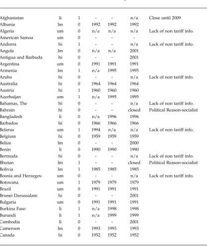
1.1 KeyIndicators ofLandlockedCountries in2007 . . . 6
2.1 Summary ofLiteratureSurvey . . . 21
2.2 GrowthDeterminants: AllCountries1980-2009 . . . 43
2.3 GrowthDeterminants: All countries1996-2009 . . . 44
2.4 GrowthDeterminants: All countries1996-2009withGovernance 45 2.5 GrowthDeterminants: AllDeveloping countries1980-2009 . . . . 48
2.6 GrowthDeterminants: AllDeveloping countries1996-2009 . . . . 49
2.7 GrowthDeterminants: AllDeveloping countries1996-2009with Governance. . . 51
2.8 Growth Determinants: All Developing countries 1996-2009 (5-year average) . . . 52
2.9 GrowthDeterminants: Landlocked Developing countries 1980-2009 . . . 55
2.10 GrowthDeterminants: Landlocked Developing countries 1996-2009 . . . 56
2.11 GrowthDeterminants: Landlocked Developing countries 1996-2009withGovernance . . . 58
2.12 GrowthDeterminants: Landlocked Developing countries 1996-2009withRule ofLaw . . . 59
2.13 LandlockedDeveloping countries1996-2009withGovernance*Resources 60 2A.1 Details ofCountries covered andUpdatedSachs-Warner index . 63 2A.2 DescriptiveStatistics . . . 69
2A.3 CorrelationMatrix . . . 70
2A.4 GrowthDeterminants: All countries1980-2009withTrade/GDP 71 2A.5 GrowthDeterminants: All countries1980-2009with SWWWin -dex . . . 72
3.1 Average RegionalTariffStructure inDevelopingCountries(%) . 78 3.2 LiberalizationStatus: LandlockedDevelopingCountries . . . 80
3.3 Trade percent ofGDPonAverage: LLDCs . . . 82
3.4 ExportPolicy andLogisticIndicators . . . 86
3.5 Export%ofMerchandise in1999, 2007and2009 . . . 92
3.6 ExportsDynamics inLLDCs"RCA>1" . . . 98
3.7 AugmentedGravityModel: DevelopingCountries . . . 112
3.8 Augmented Gravity Model:PPML Estimation-Developing Coun -tries . . . 113
3.9 Augmented Gravity Model:PPML Estimation-Developing Coun -tries . . . 115
3.10 Augmented Gravity Model:PPML Estimation-Developing Coun -tries . . . 116
3.11 Augmented Gravity Model:PPML Estimation-Developing Coun -tries . . . 117
3A.1 Top20 RCA Products forLLLDCs in2010 . . . 120
3A.2 DescriptiveStatistics . . . 133
3A.3 CorrelationMatrix . . . 134
3A.4 Exports, Landlockedness,trade costs and tariffs . . . 135
3A.5 BasicGravityModel: DevelopingCountries . . . 136
4.1 SectoralValueAdded%ofGDP . . . 148
4.2 TariffRates: Comparison withIndia(in%) . . . 150
4.3 InternationalTrade ofNepal(US$ Million) . . . 155
4.4 Non-garment exports fromNepal(MillionUS$) . . . 159
4.5 Exports growth inNepal, LLDCs andWorld,average(%) . . . 161
4.6 TotalMerchandizedExports and share inLLDCs . . . 161
4.7 Nepal inWorldExports . . . 164
4.8 Top15 Destinations ofNepalese exports . . . 166
4.9 Nepal: SITC 3digitCommodity composition of Exports inUS$000 . 169 4.10 Exports ofNepal:RCA>1 SITC Revision2data . . . 170
4.11 Commodities exported toIndia fromNepal . . . 171
4.12 Major Products Exported to India and Imported from World US$000 . . . 172
4.13 VariableConstruction andDataSources. . . 179
4.14 Determinants ofExportPerformance1980-2010 (RandomEffect -year) . . . 182
4.15 Exports toWorld1980-2010 (RandomEffect) . . . 185
4.16 Exports toIndia 1980-2010 (RandomEffect) . . . 188
4.17 Exports toRest ofWorld(ExcludingIndia)1980-2010 (RandomEf -fect) . . . 189
4.19 Robustness CheckREresults, Exports to other thanIndia 1980-2010 . . . 191 4A.1 DiscretionaryChange in the exchangeRate ofNRe vis-à-visIRe . 194 4A.2 DescriptiveStatistics . . . 195 4A.3 CorrelationMatrix . . . 196 4A.4 Determinants ofExportPerformance toWorld1980-2010 (POLS) . 197 4A.5 Determinants ofExportPerformance toIndia1980-2010 (POLS) . 198 4A.6 Determinants ofExportPerformance to rest ofWorld1980-2010
ADB Asian Development Bank AFC Asian Financial Crisis CA Republic Central African Republic CBS Central Bureau of Statistics
CEPII Centre d’Etudes Prospectives et d’Informations Internationales COMTRADE Commodity Trade Statistics Database
CPN Communist Party of Nepal
DCs Developing Countries
EAM East Asian Miracle
EAP East Asia and Pacific
ECA Eastern Europe and Central Asia ECB European Central Bank
ECN Election Commission of Nepal
Exp. Export
exp. Exponential
FDI Foreign Direct Investment
FE Fixed Effect
FGLS Feasible Generalized Least Squares GATT General Agreement on Tariffs and Trade GDP Gross Domestic Product
GDPPC Gross Domestic Product per capita GFC Global Financial Crisis
GNI Gross National Income
Gov Governance
GPML Gamma Pseudo Maximum Likelihood HDI Human Development Indicator
HS Harmonized Commodity Description and Coding System
HT Hauseman Taylor
ICD Inland Clearance Depot IMF International Monetary Fund
IRe Indian Rupee
IV Instrumental Variables
Kg. Kilogram
LAC Latin America and Caribbean LLDCs Landlocked Developing Countries
MA Market Access
MFA Multifibre Agreement MSN Market Size in Neighbor
NBER National Bureau of Economic Research
NC Nepali Congress
NIEs Newly Industrialized Economies NLS Non-linear Least Squares
NRe Nepalese Rupee
NTB Non-tariff Barrier OLS Ordinary Least Squares
POLS Pooled Ordinary Least Squares PPML Poisson Pseudo Maximum Likelihood RCA Revealed Comparative Advantage
RE Random Effect
RTA Regional Trade Agreement
SGMM System Generalized Method of Moments SITC Standard International Trade Classification
SSA Sub-Saharan Africa
SWI Sachs-Warner Index
UML Unified Marxist and Leninist
UN United Nations
UNCTAD United Nations Conference on Trade and Development
US United States
US$ United States Dollar
USSR Union of Soviet Socialist Republics
WB World Bank
WDI World Development Indicators WGI World Governance Indicators WITS World Integrated Trade Solution WTO World Trade Organisation
WWI Wacziarg-Welch Index
Introduction
“The gains from trade depend on the transport costs between a national economy
and the rest of the world being low enough to permit an extensive interaction
be-tween the economy and world markets. If the economy is geographically isolated–
for example, landlocked in the high Andes or the Himalayas or Central Africa,
as in the cases of Bolivia, Nepal, and Rwanda–the chances for extensive trade are
extremely limited.”
-Jeffrey Sachs (Sachs 1998, P. 101)
1
.
1
Context
This thesis was motivated by the casual observation that there is something pecu-liar about the common fate of landlocked developing countries when it comes to their growth and trade performance. It is hypothesised that the landlockedness, the geographical situation of a country without direct access to the sea, imposes exoge-nous costs resulting in poor economic and trade outcomes.1 The history of economic growth also suggests that landlocked countries have grown much more slowly than countries with access to the sea or navigable rivers. There is also a big difference
be-1The term ’landlockedness’ refers to the state of being landlocked, and is widely used in
tween per capita GDP of landlocked developing countries and the rest of developing countries.2
Among the 214 countries and territories in the world, 44 are landlocked. The landlocked countries comprise about eight percent of the world’s population, but account for less than one and a half percent of world GDP. Only nine of the 44 landlocked countries are high income countries (these are defined as landlocked developed countries in this study). The remaining landlocked countries belong to low income, lower middle income and upper middle income categories: these are defined as landlocked developing countries (LLDCs) in this study. The LLDCs ac-count for less than one half of one percent of the world’s GDP, but contain about three and a half percent of the world’s population. The figures show that these coun-tries are among the poorest of the poor and a high proportion of the bottom billion, live in these countries with a low living standard (Collier 2007). Two specific fea-tures of LLDCs commonly referred to in the literature as being a reason for their poor economic performance are: comparatively higher trade costs resulting from landlockedness, and they are surrounded by other poor countries depriving them of positive neighbourhood benefits (such as growth spill over or decent infrastruc-ture and poor transits). Against this background, United Nations (2006), Arvis et al. (2007) and World Bank (2013) suggest promoting an efficient transit system to lower the transaction costs in landlocked countries. However, there are notable differences of economic growth and trade performance records among these countries.
In the literature on economic growth and development, landlockedness is commonly treated as a constraint specific to developing countries. If a country is surrounded by rich countries, the impact of landlockedness is minimal, in fact, it can
2World Bank classification based on 2009 GNI per capita measured in US$; low income countries
even be an advantage to be located within a rich neighbourhood (Collier & Gunning 1999b, Collier & Gunning 1999a, Gallup et al. 1999, MacKellar et al. 2000, Dollar & Kraay 2003, Arvis et al. 2007, Grigoriou (2007). Sachs 2008, Friberg & Tinn 2009). However, so far no systematic attempt has been made to examine determinants of differences in growth performance among landlocked countries.
This thesis is focused only on landlocked developing countries because the nine landlocked developed countries are surrounded by other developed countries in Western Europe with access to one of the best trade networks in the world. Their challenges, therefore, are quite distinct from those faced by LLDCs in terms of geog-raphy and stage of economic advancement.3 The process of economic transformation triggered by the Industrial Revolution spread to these landlocked developed coun-tries before the present political boundaries came into existence. Well before the time when economic development of ‘less-developed’ (subsequently renamed ‘de-veloping’) countries became a key policy emphasis both at national and international levels in the post-war era, these nine countries had gained the status of ‘developed’ countries. Thus, the contemporary policy debate on landlockedness as a constraint on economic development is specifically related to the landlocked developing coun-tries (LLDCs).
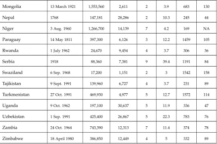
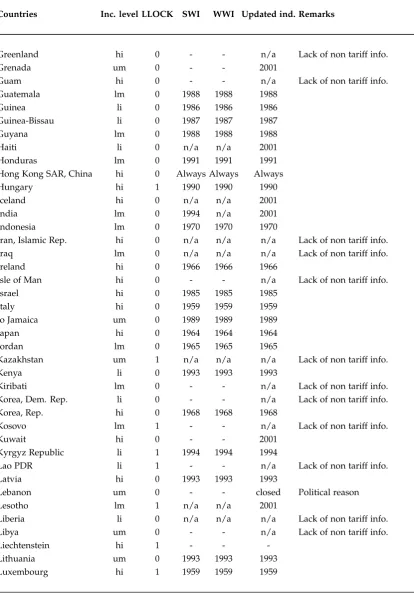
The LLDCs are scattered in different regions: two in East Asia and the Pa-cific (EAP), 12 in Eastern Europe and Central Asia (ECA), two in Latin America and the Caribbean (LAC), three in South Asia (SA), and 15 in Sub-Saharan Africa (SSA). Figure 1.1 shows the map of the landlocked countries in the World with some special differences among the landlocked countries (two countries, Uzbekistan and Liechtenstein are double landlocked, that is, locked by other landlocked countries; and two countries, Lesotho and San Marino each are locked by a country, that is,
3These nine countries are: Andorra, Austria, Switzerland, Czech Republic, Hungary, Liechtenstein,
Pacific Ocean Pacific
Ocean
Atlantic Ocean
Indian Ocean
Landlocked developed countries Landlocked developing countries Double landlocked countries
N
Liechtenstein
San Merino
Uzbekistan
Lesotho See inset map
Country Indpdc. Date Area
Sq.Km.
Population
(’000)
Nbrs. GDP
(US$
Bln.)
RGDPPC Trade /
GDP %
Afghanistan 19 Aug. 1919 652,230 28,259 7 9.7 NA 77
Armenia 23 Sep. 1991 28,480 3,072 5 9.2 1425 58
Azerbaijan 30 Aug.1991 82,620 8,581 6 33 1946 96
Belarus 25 Aug. 1991 202,900 9,702 5 45.3 2255 128
Bhutan 8 Aug. 1949 38,390 676 2 1.2 1178 103
Bolivia 6 Aug. 1825 1,083,300 9,524 5 13.1 1125 76
Botswana 30 Sep. 1966 566,730 1,892 4 12.4 4233 83
Burkina Faso 5 Aug. 1960 273,600 14,721 6 6.8 260 NA
Burundi 1 July 1962 25,680 7,837 3 1 110 NA
CA Republic 13 Aug. 1960 622,980 4,257 5 1.7 231 37
Chad 11 Aug. 1960 1,259,200 10,622 6 7 285 107
Ethiopia 2000 years 1,000,000 78,646 6 19.2 176 45
Hungary 1001 89,610 10,055 7 139 6168 159
Kazakhstan 16 Dec. 1991 2,699,700 15,484 5 105 2332 92
Kosovo 10 June 1999 10,887 1,785 4 4.7 1594 69
Kyrgyz Republic 31 Aug. 1991 191,800 5,234 4 3.8 353 133
Lao PDR 19 July 1949 230,800 6,092 5 4.3 451 87
Lesotho 4 Oct.1966 30,360 2,031 1 1.6 455 164
Macedonia, FYR 17 Sep. 1991 25,230 2,039 5 7.9 2077 126
Malawi 6 July 1964 94,080 14,439 3 3.5 152 62
Mali 22 Sep. 1960 1,220,190 12,408 7 7.2 292 62
Table 1.1 Continue
Mongolia 13 March 1921 1,553,560 2,611 2 3.9 683 130
Nepal 1768 147,181 28,286 2 10.3 245 44
Niger 3 Aug. 1960 1,266,700 14,139 7 4.2 169 NA
Paraguay 14 May 1811 397,300 6,126 3 12.2 1459 105
Rwanda 1 July 1962 24,670 9,454 4 3.7 306 36
Serbia 1918 88,360 7,381 9 39.4 1191 84
Swaziland 6 Sep. 1968 17,200 1,151 2 3 1542 158
Tajikistan 9 Sept. 1991 139,960 6,727 4 3.7 231 89
Turkmenistan 27 Oct. 1991 469,930 4,977 5 12.7 1572 114
Uganda 9 Oct. 1962 197,100 30,637 5 11.9 336 47
Uzbekistan 1 Sep. 1991 425,400 26,867 5 22.3 783 76
Zambia 24 Oct. 1964 743,390 12,313 7 11.4 374 78
Zimbabwe 18 April 1980 386,850 12,449 4 5 332 89
Note: Indpdc. Date refers to Independence date/ country foundation date where applicable taken from McLachlan (1998), Nbrs. refers to number of neighbouring countries, RGDPPC is real per capita GDP measured in US$ base year 2000, GDP also has the same base year, Lesotho is locked by South Africa.
Sources: Based on data compiled from World Bank (2010) and other sources as in the footnotes.
1
.
2
Purpose and Scope
among LLDCs that goes beyond inferring “average” results for all landlocked coun-tries. This is an important gap in the growth literature because there is great hetero-geneity in development experiences among landlocked developing countries. This thesis seeks to fill this gap. Understanding the divergences in economic performance among these countries and the underlying causes can greatly enrich the policy dis-course in these countries and in the international development community.
The purpose of this thesis is three-fold. Each of these is addressed in the three core chapters: first, to examine empirically the impact of landlockedness on eco-nomic growth through analysing the difference between LLDCs and non-landlocked developing countries; second, to examine the impact of landlockedness on export performance of developing countries by identifying the differences between LLDCs and non-landlocked developing countries group; and third, to examine the determi-nants of export performance of one LLDC, Nepal, as a case study.
1
.
3
Overview
Chapter 2, the first paper, makes a number of contributions. The primary contribu-tion of this chapter is the new strategies employed to identify the differences among LLDCs and other developing countries from country-level panel data. The estima-tions control for country-specific fixed and random effects follows the instrumental variable based technique as developed in Hausman & Taylor (1981) [HT]. As part of the empirical analysis of the chapter, I also updated the trade liberalisation index, originally developed by Sachs & Warner (1995), up to 2009 following Wacziarg & Welch (2008), thereby extending the number of countries covered from 141 to 197.
The results from this chapter confirm the findings of previous studies that landlockedness hampers economic growth, although the magnitude of the negative impact is sensitive to alternative estimation methods. In addition, there is evidence that a good governance system and sound policy initiatives can help lower the neg-ative impact of the constraints imposed by landlockedness. Openness is positively associated with economic growth in landlocked countries, suggesting that the more open a country is to foreign trade, the higher its growth prospects are. In addi-tion, the economic development of neighbouring countries is one of the major de-terminants of economic growth in LLDCs. It appears that coordinating the devel-opment tasks with neighbours’ infrastructure may be a useful means of improving the development prospects of LLDCs. There is also strong evidence that, in terms of economic growth performance, landlocked developing countries in Africa are not different from other LLDCs.
Pseudo Maximum Likelihood (PPML) which was found to be superior to pooled ordinary least square (POLS), Random Effect (RE), Fixed Effect (FE) and Hausman-Taylor (HT) estimations in terms of the standard tests.
The results suggest that, while landlockedness remains a specific constraint on export performance, LLDCs have opportunities to improve their export perfor-mance by creating a more trade-friendly environment through lowering tariffs, re-forming exchange rates and involving themselves in regional trade agreements. The results for the relative factor endowment variable confirm the Linder hypothesis, which suggests that trade links are much stronger among countries with similar income levels. Distance-related trade costs restrict export performance more in land-locked developing countries than in other developing countries. Having a common border with an influential trading partner is more important than having a common language with them for export performance in LLDCs. There is evidence to suggest that African landlocked countries’ export levels are at least 30 percent higher than the average level for other LLDCs.
for export competitiveness with third countries; and the differences in import tariffs between the two countries which create trade deflection in Nepal. The principal estimation technique used in this chapter is random effect (RE) which was found to be superior to pooled ordinary least square (POLS), Fixed Effect (FE) and Hausman-Taylor (HT) and Poisson Pseudo Maximum Likelihood (PPML) estimations in terms of the standard tests.
The results demonstrate that the high land transport costs, which are beyond the control of the country given its landlockedness, exert a significant constraint on Nepal’s export performance. Therefore, identification of specific product types that accelerate export growth is an important policy issue. Related to this, a major finding of this chapter is that value-to-weight ratio has a strong positive relationship with inter-product differences in export performance. This implies that Nepal has the potential to promote exports of high-value-to-weigh products such as tea, coffee, spices, and apparel.
Landlockedness and Economic
Growth: New Evidence
Summary
This chapter examines the determinants of economic growth, with emphasis on the experience
of landlocked developing countries. When landlocked countries are treated as a group within
the standard growth regression framework, the results confirm the findings of previous
stud-ies that landlockedness hampers economic growth, although the magnitude of the negative
impact is sensitive to alternative estimation methods. However, the country level analysis
suggests that good governance and openness to foreign trade can explain a significant aspect
of the inter-country differences among LLDCs. Contrary to the ’resource curse’ hypothesis,
the results suggest that natural resources contribute significantly to the economic growth of
landlocked countries. It appears that coordinating the development tasks with neighbours’
infrastructure may be a useful means to improve the development prospects of landlocked
2
.
1
Introduction
This chapter examines the determinants of economic growth in developing countries, with special attention being paid to the experience of landlocked countries (LLCs). Landlockedness has been widely identified as a constraint on economic growth in the empirical growth literature (Bowen 1986, Srinivasan 1986, Collier & Gunning 1999b, Collier & Gunning 1999a, Gallup et al. 1999, MacKellar et al. 2000, Dollar & Kraay 2003, Arvis et al. 2007, Sachs 2008 and Friberg & Tinn 2009). Most of these studies have examined the impact of landlockedness on growth within the multi-country growth regression framework using a binary dummy (1 if country is landlocked and 0 if a country is not landlocked) and found that when controlled for the other relevant determinants, on average the growth rate of landlocked countries is three and a half percentage points lower than that of other countries.
This chapter aims to broaden the understanding of the above issue in two ways. First, it examines the robustness of the findings of the previous studies on landlockedness to alternative estimation methods. Second, and more importantly, it probes the determinants of inter-country growth differentials among landlocked de-veloping countries. The focus of the analysis is to address the questions of whether or not the landlockedness is a root cause of economic backwardness, and whether ap-propriate economic policies can help to achieve faster growth within the constraints set by landlockedness. In order to address these questions, this chapter aims to de-lineates policy-related factors from other factors that explain differences in economic growth among landlocked countries.
countries) and the rest are low income and middle income countries (landlocked de-veloping countries, LLDCs)World Bank (2010).1 The majority of these countries are in
the “bottom billion” as defined by Collier (2007). In 2009, the average real per-capita gross domestic product of LLDCs was US$974, compared to US$2,392, the GDP of non-landlocked developing countries.2 The LLDCs’ share of world trade was a mere one percent compared to 27 percent for non-landlocked developing countries, and notably, both per capita trade and GDP are low in LLDCs. These data partly reflect the strong positive nexus of trade and growth in these countries. Not all landlocked developing countries are in a similar phase of economic development, some coun-tries have upper middle income levels and some are in the low income category. Noting this gap in the literature, this study examines how the main determinants of growth identified in the empirical growth literature play different a role in land-locked developing countries. To my knowledge, this is the first study to examine the determinants of inter-country differences in growth rates of landlocked countries. This study also updates the Sachs-Warner index of liberalisation, extending both the number of countries and time period covered in the index. The numbers of coun-tries were extended from 141 to 197; and the time coverage from 1999 to 2009. (see Table 2A.1 for details).
The empirical analysis is based on an unbalanced panel data set, for the period 1980 to 2009 for the “all developing countries” group (143 countries) and for the period 1996 to 2009 for the “landlocked developing countries” (34 countries). After testing alternative panel estimation techniques, the Hausman-Taylor estimator is the preferred method. The results confirm the findings of previous studies, that landlockedness hampers economic growth, but also reveal that the magnitude of the
1World Bank classification based on 2009 GNI per-capita measured in US$; low income countries
$995 or less (17 LLDCs); lower middle income $996 - $3,945 (10 LLDCs); upper middle income, $3,946
- $12,195 (7 LLDCs); and high income above $12,195 (9 LLDCs )World Bank (2010).
2Data reported in this chapter, unless otherwise stated, are from the World Development Indicators
negative impact is much larger than in the literature. Good governance and open-ness to foreign trade seem to explain inter-country differences in growth rates among LLDCs, suggesting that landlockedness is not destiny. The results also suggest that the African landlocked countries are not different to other landlocked developing countries in terms of economic growth. There is also evidence that the level of de-velopment of the neighbouring countries has a significant impact on the economic growth of a given landlocked country. Therefore, coordinating development tasks with the neighbouring countries’ infrastructure may be a useful means of improv-ing the development prospects of landlocked developimprov-ing countries. Contrary to the “resource curse” hypothesis, the results suggest that natural resources rents seem to contribute significantly to economic growth in landlocked developing countries.
The chapter is structured in six sections. Section 2.2 presents a brief lit-erature survey of landlockedness and economic growth. Section 2.3 provides an overview of landlocked economies to set the context for the ensuing analysis. Sec-tion 2.4 takes a closer look at neighbourhood impact on landlocked countries. SecSec-tion 2.5 discusses model specification, data sources and variable construction, and the es-timation method. Section 2.6 presents and interprets the results. The final section summarizes the key findings and draws policy inferences.
2
.
2
Brief Literature Review
There is a vast literature on the determinants of economic growth.3 This section
undertakes a selective survey of this literature. The selection is guided by the di-rect relevance for the model specification and variable construction in the ensuing
3Sala-I-Martin (1997), Barro (1999), and Acemoglu (2009)-Chapter 1 for detail surveys of his
empirical analysis.
Some studies have attempted to identify and analyse the impacts of land-lockedness. The cross country studies include Srinivasan (1986), Gallup et al. (1999), Collier & Gunning (1999a), MacKellar et al. (2000), Carrere & Grigoriou (2008) and Friberg & Tinn (2009). Hailou (2007) investigated the spatial constraints; however, more attention is given to the role of geographic conditions such as regional and tropical constraints on economic growth. These studies examine some aspects of the economic performance of landlocked countries using multi-country cross-sectional data. In the aggregate-level studies, most landlocked developing countries are not included and the methodology and data need to be updated. Many of the studies use a landlockedness dummy in the empirical literature, and conclude that this dummy variable has a statistically significant negative impact on economic growth.
So far only few country level studies are in the context of the economic growth of landlcoked developing countries, for example: Paudel & Shrestha (2006) studies on the role played of external debt, total trade and labour force in Nepal, a landlocked country, and found that trade openness is an important contributor to the economic performance of the country. Bird & Hill (2010) studies on Laos to evalu-ate reform’s impacts on economic development and concluded that neighbourhood effects have a favourable impact on Laos economy. But this not always the case, a cautious approach should therefore be taken. Allaro (2012) studies on the export-led growth strategy of another landlocked country, Ethiopia. Menon & Warr (2013) stud-ied on another landlocked country, the Lao PDR, analysing on how the exports of the natural resources can be linked to improve the living standard of its people. How-ever, these studies have simply presented a historical narrative and do not attempt a systematic empirical analysis to identify the impacts of landlokedness.
slows the growth process. However, none of the studies have covered all the land-locked countries in the sample to obtain more concrete results. In addition, these studies have not disaggregated the landlocked countries into developed and devel-oping countries, and many if not most of them use narratives rather than the quan-titative research methods . This chapter aims to bridge this gap in the literature by disaggregating the developing countries into landlocked and non-landlocked devel-oping countries so that the real impacts of landlockedness on poor countries can be identified.
The existing literature shows that the determinants of economic growth are not the same in all countries. The theory of economic growth has been developed through the contributions of many scholars. Solow (1956) contributed to the theory of economic growth emphasising the role of investment, saving and employment in the economy. A large number of studies attempted to identify the determinants of economic growth in different countries. The studies in the literature analyzed the determinants of economic growth with different focuses; Barro (1999) analyzed the determinants of economic growth and concluded that better maintenance of the rule of law, lower inflation, smaller government consumption, initial level of GDP, and the initial level political right influence growth but growth tends to become retarded after a moderate level of democracy is obtained.
& Williamson (2004), Kalirajan & Singh (2008), Awokuse (2008), Paudel & Perera (2009) and Dufrenot et al. (2010) concluded that trade has contributed substantially to economic growth in recent decades in many ways. The data show that the role of trade 50 years ago was not as important as it is today. Athukorala (2011) suggests that network trade helps towards faster integration and economic interdependence within the region, which is an important process benefitting from trade by creating employment and extending output in this era.
The price of investment goods, distances to major world cities, growth pro-moting policy strategies, quality of access to international markets, and institutional reforms are the determinants of economic growth as pointed by Moral-Benito (2009). The role of institutional quality is doubtlessly important to manage the resources in a meaningful way as argued by North (1987), Acemoglu et al. (2001), Glaeser et al. (2004), and recently Brunnschweiler (2008). Many scholars have further focused on the growth process; Temple (1998) attempted to identify the adverse effects of bad policy outcomes in African countries, considering initial conditions that account for more than half of the variation in developing countries’ growth rates, using the least trimmed squares method for cross country data. Temple concluded that developing countries with relatively low social capital have poor policy outcomes, resulting in low investment and growth.
government to invest in infrastructure; and the ability to adapt international tech-nology to local ecological conditions; macroeconomic stability; and the quality of governance are the key elements of economic development identified by Sachs.
Landlockedness and Economic Growth
Author (Year). Title Methodology /Data Findings/Conclusions
Friberg & Tinn (2009). “Land-locked Countries and Holdup”
GE modeling and gravity equation using the trade data of land-locked countries from 1950 to 2000.
Potential for holdup (the problem caused by the
landlockedness) reduces trade by more than 50 percent and free trade agreements with transit countries have only a weak effect on trade.
Arvis et al. (2007). “The Cost of being land-locked: Logistics Cost and Supply Chain Reliability”
Microeconomic quantitative description of logistic cost
Land-locked countries are affected by high costs of freight services, high degree of unpredictability of transport system.
MacKellar et al. (2000). “
Economic Development Problems of land-locked Countries”
Regression Analysis for 92 developing countries from 1980 to 1996.
Gallup et al. (1999). “Geography and Economic Development”
Empirical Analysis (AK Model-Harrod Domar Model) using some comparative data from different points in time from 1950 to 1990.
from coasts and ocean-navigable rivers have to bear heavy transport costs of international trade. Tropical regions are also disadvantaged because of disease burden. Geographically disadvantaged regions will have higher population growth over the next three decades. Coastal countries have higher incomes than land-locked countries.
Srinivasan (1986). “The Costs and Benefits of Being a Small, Remote, Island, Land-locked, or Mini state Economy”
Qualitative Analysis
Absence of economies of scale, vulnerability, remoteness, reduced access of capital markets, macroeconomic policy dependence are the major problems in small economies.
Determinants of Economic Growth (Selected Studies)
Dufrenot et al. (2010). “The Trade-growth Nexus in the Developing Countries: a Quantile Regression Approach”
Quantile regression analysis of cross-section annual data from 75 developing countries for the duration of 1980-2006.
Arora & Vamvakidis (2005). “How Much Do Trading Partners Matter for Economic Growth?”
Panel estimation for 101 industrial and developing countries from 1960 to 1999.
Trading partners’ economic growth plays a significant role in the economic growth of a country.
Rodrik et al. (2004). “Institutions Rule: The Primacy of Institutions Over Geography and Integration in Economic Development”
Instrumental variable (IV) estimation for institution and trade in income level in 79 and 137 countries for the year 1995.
Institution quality of a country is the most significant variable for its income level. If institutional quality of a country is controlled, geography and trade have less role to play in growth.
Dollar & Kraay (2003).
“Institutions, Trade and Growth”
Ordinary Least Squares (OLS) and IV estimation on large cross-section data for different periods from 1970s to late 1990s.
Investigation” economic performance.
Collier & Gunning (1999b). “Why
Has Africa Grown Slowly ?” Qualitative analysis.
Africa’s slow growth during 1970s-1990s is due to policies which reduced the region’s openness to foreign trade. Poor delivery of public services is the main hurdle of economic growth in the region, an investment-friendly environment needs to be initiated.
Frankel & Romer (1996). “Trade and Growth: An Empirical Investigation”
IV estimation with measure of geographic component of countries’ trade (OLS with IV estimation) using trade data for 63 countries.
Countries’ geographic characteristics have significant effects on their trade, and significant and robust effects on income.
Levine & Renelt (1992). “A Sensitivity Analysis of Cross-Country Growth Regressions”
Sensitivity Analysis for 119 countries covering the period 1960-1989
depending on data availability.
Economic Growth”
Barro (1991). “Economic Growth in a Cross section of Countries”
Used Regression Analysis of data on 98 countries covering annual data from 1960 to 1985.
Positive association between initial level of education and political stability, and growth. Negative
2
.
3
Landlocked Economies: An Overview
In terms of land area, Kazakhstan is the largest landlocked country, and Ethiopia has the largest population (almost 78 million) (Table 1.1 , Chapter 1). Different trends of population growth are seen, Niger has almost four percent annual population growth, while Belarus, Moldova, Serbia and Zimbabwe have negative population growth . Presumably because of high trade costs, LLDCs are not well integrated with the rest of the world to benefit from globalization. Most LLDCs have very low trade to GDP ratios. Azerbaijan has recorded the highest growth in recent decades while Turkmenistan and Afghanistan have an average of more than 10 percent growth; in contrast, Zimbabwe has had an average of negative six percentage growth rate for the same period. Afghanistan, Azerbaijan, Burkina Faso, Chad, Ethiopia, Mali, Niger, Serbia and Zambia are surrounded by more than five countries each, and Serbia has the maximum number (nine) of neighbours.
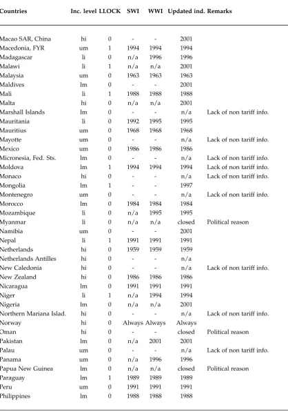
The differences in per capita GDP between landlocked and non-landlocked developing countries are illustrated in Figure 2.1. The average per capita GDP of the former in 2009 was less than US$1000, compared to well above US$2000 in the latter. The average per capita GDP of non-landlocked developing countries ramained consistently higher over the period from 1980 to 2009.
Figure2.1: Real per-capitaGDP- DevelopingCountries
0
2000
4000
6000
GDP per capita US$
1980 1985 1990 1995 2000 2005 2010
Year
Non−Landlocked Developing Countries Landlocked Developing Countries World
Source: Based on data compiled from WDI, World Bank (2010).
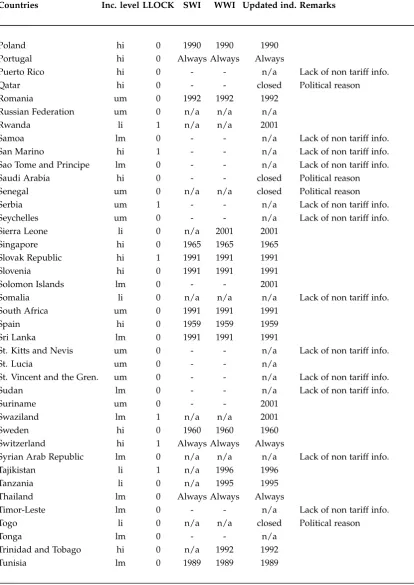
Figure2.2: Trade-Growth relationship-developing countries in2009
BRA CHL CHN GAB IND KNA LBN LCA MDV MEX MUS MYS PAN RUS TUR URY VEN ZAF ARM AZE BLR BWA KAZ MKD SRB SWZ TKM 0 5000 10000 15000
Per Capita Trade $
0 5000 10000 15000
Per Capita GDP $
Non−Landlocked Landlocked Fitted values
2
.
4
Neighbourhood Impact on Landlocked Economies
The ’neighborhood effect’, defined as the spillover effect of neighboring countries’ economic performance on a given country, has been used in some recent studies as a determinant of inter-country differences in economic growth (Easterly & Levine (1998), Arora & Vamvakidis (2005), Collier & O’Connell (2007) and Roberts & De-ichmann (2011)). Presumably this variable is much more important for the deter-mination of growth performance of landlocked countries compared to the other de-veloping countries for two reasons. First, trade cost faced by a landlocked country depends crucially on the quality of trade-related infrastructure of the neighbouring country through which it conducts international trade. Secondly, given this excessive trade cost, the geographic profile of trade of a landlocked country is likely to have a neighbourhood bias.
2.4.1 Market Size
MSNi,t= [ n
∑
j=1
βjXj,t] (2.1)
where,
MSN refers to market size in the neighbours of a landlocked developing countryi,
βrefers to the weight of neighbour country’s trade to world trade,
Xis the GDP of the neighbour country,
t is time period, and
jis the number of neighbours.
To remove the country size bias arising from neighbouring countries, I weighted the neighbouring countries GDP by their shares in total world trade. This index appropriately captures the market size of the neighbouring countries, as it takes into account the trading significance of each neighbouring country in addition to its economic size.
2.4.2 Market Access
Considering the role of international trade on economic growth, it is assumed that poor economic performance of landlocked countries is due to the distance from their nearest commercial port to the business capital city of the country. For this infras-tructure quality adjusted distance to port is constructed as follows:
MAi = PDi/[( n
∑
j=1
where,
MA refers to market access and is an index,
PD stands for distance to the nearest commercial port from the business capital city of landlocked country,
j refers to the number of neighbours of the landlocked country;
GDPPCR refers to the real per capita GDP of neighbours, a proxy for infrastructure quality and the phase of economic development, and
Years refers to the total number of years, which is 14 (this variable is used only for the landlocked countries group for 1996-2009).
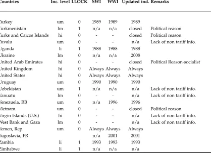
The relationship between port distance and neighbours’ economic develop-ment for landlocked countries is depicted in Figure 2.3. In this figure, X axis mea-sures the distance index constructed as pdistance= 1− (Distance to port−Minimum distance from port in the group)/(Maximum distance from port in sample−Minimum
dis-tance to port in the group); the Y axis measures the log of neighbours’ GDP in log
form as calculated in equation 2.1 above. The right top corner countries benefit most because they have very short distances to the nearest port and their neighbours have big size economies, that is, they are developed such as Andora, Czech Republic, Aus-tria, which have very favourable positions and benefits ( for reference, however, these countries are not the concern of this study). Most of the LLDCs are scattered on the other quartile. Azerbaijan is attached to a landlocked sea (Caspian Sea) and hence has more neighbours including Russia.
cor-ner suffer due to the long distance to the nearest port even though they are situated among rich neighbours such as Kyrgyz Republic, Kazakhstan, and Afghanistan.
Figure2.3: PortDistance and neighbours economies
ADO AFG ARM AUT AZE BDI BFA BLR BOL BTN BWA CAF CHE CZE ETH HUN KAZ KGZ KSV LAO LIE LSO LUX MDA MKD MLI MNG MWI NER NPL PRY RWA SMR SRB SVK SWZ TCD TJK TKM UGA UZB ZMB ZWE 15 20 25
Normalised GDP of Neighbours
0 .2 .4 .6 .8 1
Port Distance Index
Source: Based on data compiled from WDI, World Bank (2010) and http://www.findaport.com/
2
.
5
Methodology
2.5.1 Model
Solow-Swan model as specified in (2.3):
Yt =K(t)α(A(t)L(t))1−α (2.3)
where,
Yis output,
Kis capital, and
Lis labor
L and A are assumed to grow exogenously at rates n (population growth) andg(growth).
In the literature, the variables used to estimate the growth model are very diverse. Sala-I-Martin (1997) has estimated 62 explanatory variables, and identify variables (which he dubs ‘the fixed variables’) which are most relevant for growth model. I expanded the basic model (2.3) by adding these fixed variables. The full model, with the conventional notation for panel structure, takes the form:
Gi,t =γ1yt−1+γ2Capt+γ3Opent+γ4Edut+γ5Llock+γ6Nrest+ηt+µi+vi,t (2.4)
where,
yt−1= initial income, real per capita GDP int−1 to pick up convergence effects (-),
Cap =the ratio of capital formation to GDP (+),
Open= openness measured with trade as a percentage of GDP (+)
Edu=Education, mean years of schooling for the age 25 years or over (+),
Llock=Landlockedness, a binary dummy (-), and
Nres=natural resource rent to as percentage of GDP (+).
The last term vi,t is the error term and is assumed to have a normal
dis-tribution; η captures any common period-specific effect, such as general technical
progress; andµrepresents the time invariant variables. The dependent variable is in
percentage, initial income is in natural log, capital formation to GDP, trade to GDP and natural resource rent to GDP ratios are in percentages. Openness is measured with an alternative variable i.e. the updated Sachs & Warner (1995) index. This in-dex was updated following Wacziarg & Welch (2008) [SWWW inin-dex], and a binary variable. The signs ofγ1andγ5are expected to be negative, the others positive.
A second stage of analysis looks at growth rate differentials among the group of landlocked developing countries and includes three additional variables: Gov, MSN and MA:
Gi,t=γ1yt−1+γ2Capt+γ3Opent+γ4Edut+γ5Nrest+γ6Govt+γ7MSNt+γ8MA+ηt+µi+vi,t
(2.5)
where,
MSN=aggregate market size in neighbouring countries (equation 2.1) (+), and
MA=neighbours’ infrastructure-adjusted port distance (-) (equation 2.2) .
Two complementary measures are used to capture the neighbourhood effect: MSN in natural log form and MA as an index. The signs of γ1 andγ8 are expected
to be negative, the others positive. In the empirical application of equations (2.1) and (2.2), governance and market access are indexes. The sign given in the parenthesis of the variables detail are expected sign.
2.5.2 Data Sources and Variable Construction
For the econometric analysis, the data for most variables are collected from the World Development Indicators World Bank (2010). The data for port distance used to con-struct MA are accessed from www.findaport.com. The empirical tests for the locked countries are conducted only for the period from 1996 to 2009, as 14 land-locked countries were formed in the early 1990s.
Among the explanatory variables, landlockedness is measured with a binary dummy, equal to 1 if a country is landlocked and 0 if a country is non-landlocked. This way, in all countries group, landlockedness (Llock) is replaced by the dummy for landlocked developed countries, landlocked developing countries, and non-landlocked developing countries, thus allowing comparision of these three groups of countries with developed countries. In the developing countries group, landlockedness (Llock) is used as a variable to identify the differences between landlocked developing coun-tries and non-landlocked developing councoun-tries.
are available for every five years; they have been linearly interpolated into annual figures. Total trade percentage of GDP is the most widely used measure of trade openness in the empirical growth literature, but in its traditional calculation it has a major shortcoming as an indicator of the openness of an economy. Exports and imports are magnitudes measured in terms of production value, whereas GDP is a value added concept. The amount of GDP related to a unit of exports or imports varies between countries with different economic structures. For example, for a pri-mary goods producing country, the cumulated value added per unit of exports is generally much higher compared to that of an industrialized country. The propor-tion of import content in GDP varies with the economic size of the country. For these reasons, it is preferable to use a direct measure of the openness of the foreign trade regime (see Krugman 1995 and Athukorala & Hill 2010 for more detail). The ideal measure of openness would be the effective rate of protection (ERP) but these data are not available for many countries. Therefore, I use the updated Sachs & Warner (1995) index of trade liberalisation to see the sensitivity of the results.
The original Sachs and Warner binary index of trade liberalisation has been updated by Wacziarg & Welch (2008) for 141 countries for the period up to 1999, based on five major criteria. Thus, a country is liberalised when it has: average tariff rates not more than 40 percent; a black market premium rate not more than 20 percent; non-tariff barriers rates are not more than 40 percent; it does not have a state monopoly on major exports; and does not have a socialist economic system. I have updated the data for 197 countries and extended the period until 2009, using average tariff data from the World Bank. I then calculated the average for the period from 1999 to 2009. Black market premium data for the countries that are not listed in Wacziarg & Welch (2008), have been updated using Edwards et al. (2001) and the data from Global Financial data (GFDatabase 2011).4 The membership criteria of the
World Trade Organization (WTO) pave the way to proxy for non-tariff barrier data for the period after 1999. The provision is, if a country wants to become a member of the WTO, it has to virtually reduce its non- tariff barriers to zero, but if a country was a member of the General Agreement on Tariffs and Trade (GATT) prior to joining the WTO (in 1995), it was required to meet the membership conditions within a grace period of five years.5 The monopoly in the major export market was not the major determinant in the group. Based on these criteria, this index is a binary variable equal to 1 in each year after the country completes the liberalisation criteria and 0 for the period before that year.
To measure the impact of natural resources rent, natural resources rent as a percentage of GDP is used as an explanatory variable. A negative coefficient of this variable is consistent with the “Dutch Disease” theory, and a positive sign supports the hypothesis of Mehlum et al. (2006) that suggests the resource rent promotes growth.
Kaufmann et al. (2010) have developed six indices of the quality of gov-ernance, of these; the rule of law and control of corruption are considered more relevant than the other four as measures of the quality of governance in the process of economic development.6 The simple average of these two indicators is the variable used to measure the quality of governance in this paper. The simple average of the two is used instead of using the two indicators separately, because of the potential problem of high colinearity. The original data are for alternate years from 1996 to 2002. They are interpolated linearly to generate an annual series. The data for 2002 onwards are available annually.
only three countries, Afghanistan, Burundi and Zimbabwe, after 1999 in the group.
5Using this criterion, Rwanda, Tongo, Ukraine and Vietnam became liberalized after 2005, 2007, 2008
and 2007 respectively.
6These six indicators are: Voice and Accountability, Political Stability and Lack of Violence,
To capture the neighbourhood effect, previous studies used aggregate growth of the neighbouring countries (for example, Easterly & Levine (1998), Collier & O’Connell (2007) and Roberts & Deichmann (2011). As mentioned earlier in sec-tion 2.4, Roberts & Deichmann (2011) constructed an index for the spillover effect, with the weighted average growth rate of neighbours. However, neighbours’ average growth rate does not capture the development level of those neighbours, and the development level of the neighbours is more important to the growth of landlocked countries. The developed country with the highest growth rate in the neighborhood would be the best.
The neighbours’ infrastructure that matters most to a landlocked country is the access to world markets via neighbours’ ports. However, taking the average of growth in landlocked countries in this study creates a size bias in the empirical analysis and does not capture the effect of these two points, as explained in sec-tion 2.4. Hence, I calculated the variable to measure the neighbourhood effect as in equation (2.1). In addition, this paper emphasises the role of infrastructure quality in neighbouring countries with a port available for landlocked countries. For this, road and railway quality would be an important measure of infrastructure quality, but the data for road and rail service are not available for this period. Therefore, I have constructed an index of neighbours’ infrastructure quality adjusted for port distance, to measure the cost of transportation to access international markets. Equa-tions (2.1) and (2.2), respectively, show the calculaEqua-tions of the two variables related to the neighbourhood effects (see Section 2.4 for details).
2.5.3 Econometrics
& Taylor (1981). In this case, the POLS has a major problem as it ignores the panel structure of the data and assumes that the observations are serially uncorrelated (Johnston & DiNardo 1997). The FE estimator is not suitable, as the main explana-tory variable “landlockedness” is specified as a time-invariant variable in addition to the Africa dummy and market access. The RE estimator ignores the country-specific effects. The HT estimator is more effective than RE because it eliminates bias re-lated to lack of independence of the explanatory variables from the joint disturbance term. Moreover, the problem of heteroscedasticity is eliminated through the use of the general least squares method. For these reasons, the HT estimator is used as the preferred estimation method and alternative estimates using POLS, RE and FE estimations are reported for the purpose of comparison. The System Generalised Method of Moments (SGMM) developed by Arellano & Bover (1995) and Blundell & Bond (1998) is not suitable because the data set covers more than 15 years for the ’all countries’ and ’all developing countries’ group (Roodman 2009). To explain the properties of the HT estimator, consider the following stylized model:
yit=X1,itβ1+X2,itβ2+τ1β3+τ2β4+αi+εit
where, X1 and X2 are time varying regressors; τ1 andτ2 are time invarying
regressors of the model; αi is a country-specific effect, andεit is the error term. All
the regressors are assumed to be uncorrelated withεit. The relationship of regressors
with αi is assumed as cov. (αi, χ1 = 0) but cov. (αi, χ2 6= 0), cov. (αi, τ1 = 0)and
cov.(αi,τ26=0). The FE model cannot estimateβ3andβ4and the RE ignores the role
of country-specific effectαi .
address the endogeneity issue by setting the instrument as the difference between the regressor and mean of the regressor. i.e. χ1,it−χ1i (Verbeek 2008, Breusch et al.
1989, Hausman & Taylor 1981). The HT estimator gives more consistent and efficient results when more than one time invariant variables are used in the model (Cameron & Trivedi 2009). In sum, the advantage of employing HT estimation in this study are: first, it is suitable in case of time invariant variables such as landlockedness, second, it deals with endogeneity issue to make more reliable results, and third, it has the combine strength of both FE and RE.
2
.
6
Results
Descriptive statistics and the correlation matrix of the variables are presented in Ta-ble 2A.2 and TaTa-ble 2A.3 in Appendix 2A, respectively. The regression estimates are presented in Tables 2.2 to 2.12 classified into all countries, developing countries and landlocked developing countries groups. Table 2A.4 and Table 2A.5 in Appendix 2A present the results with POLS, RE, FE and HT for comparison. The post estimation statistics are presented in the lower panel of tables.
2.6.1 All Countries
Tables 2.2 to 2.4 present the growth equation estimated using the HT method for the all countries group with the base dummy of developed countries. All the estimations in these tables are compared with the developed countries disaggregated into land-locked developed countries, landland-locked developing countries and other developing countries. The main objective of doing this is to examine whether the landlocked developing countries are the most disadvantaged group in the sample. The results suggest that the level of growth is lower in all developing countries as a group com-pared to developed countries, but among the developing countries the subgroup of landlocked countries is the most disadvantaged group. The coefficient of the dummy variable for landlocked developed countries is not statistically significant; this result suggests that these countries are not different from the other developed countries. This supports the argument for focussing specifically on landlocked de-veloping countries in examining the impact of landlockedness on economic growth, as is done in this thesis. The results suggest that landlocked developing countries’ growth is lower by about 14 percentage points compared to that of developed coun-tries, holding other variables in the model constant.
of the potential endogenous variables, such as trade as percentage of GDP, gover-nance, natural resources rent as percentage of GDP, and education.
Table 2.2 presents the results for the period 1980 to 2009. The results for trade openness measured by trade as a percentage of GDP are highly significant suggesting that a ten percent increase in trade to GDP ratio increases the economic growth on average by 0.30 percentage points, holding other variables constant in the model. The coefficient of the Sachs-Warner index (SWWW) is highly statistically significant and suggests that on average the rate of growth of countries with a liber-alised trade grow two and a half percentage points faster than those with controlled trade regimes.
The results for education variable suggest that an additional year of school-ing results in an increase in the annual per capita growth rate by an average of one and a half percentage points. The coefficient of initial income variable is consistent with the growth convergence hypothesis. The coefficient for the Africa dummy is statistically significant, with the expected negative sign, only while controlled to the Sachs Warner index of trade liberalisation, and the results supports the findings of previous studies that is, on average, the annual growth rate of per capita GDP of an African country is two and a half percentage points slower than that of developed countries. The natural resources rents seem to contribute statistically significantly to growth, supporting Mehlum et al. (2006). The variable “capital formation” is also highly statistically significant, with the expected sign. The results in these tables show that the negative impacts of landlockedness are much bigger in the developing countries.
openness measured by trade as a percentage of GDP have maintained the same level of significance statistically. The Sachs Warner index coefficients are significant but the magnitudes are smaller than those shown in Table 2.2. The coefficients for education are also smaller. The results suggest that a country in Africa grows more slowly by about five percentage points on average compared to other developed countries, holding other variables constant.
Table2.2: GrowthDeterminants: AllCountries1980-2009
Hausman-Taylor Estimations,Dependent Variable: Growth of Per Capita GDP
Variables (1) (2) (3) (4)
Trade Openness (Trade% of GDP) 0.029*** 0.029***
(0.004) (0.004)
Trade Openness (SWWW) 2.446*** 2.445***
(0.253) (0.253)
Education (Edu) 1.461*** 1.461*** 1.210*** 1.209***
(0.098) (0.098) (0.103) (0.103)
Initial Income (Yt-1) in log -6.650*** -6.648*** -5.979*** -5.977***
(0.406) (0.406) (0.398) (0.398)
Capital Formation (Cap)% of GDP 0.185*** 0.185*** 0.195*** 0.195***
(0.014) (0.014) (0.014) (0.014)
Natural Resources Rent (Nres) % of GDP 0.056*** 0.056*** 0.077*** 0.077***
(0.013) (0.013) (0.012) (0.012)
Africa (Dummy) -2.176 -2.179 -2.268* -2.270*
(1.333) (1.339) (1.201) (1.204)
Landlocked Developed Economies -2.481 -1.821
(2.752) (2.463)
Landlocked Developing Economies -15.590*** -15.251*** -14.305*** -14.060***
(1.992) (1.959) (1.835) (1.803)
Non-landlocked Developing Economies -9.750*** -9.418*** -9.263*** -9.021***
(1.520) (1.475) (1.393) (1.352)
Number of observations 3,790 3,790 3,824 3,824
F Statistic 64.11 72.12 70.78 79.63
Sargan-Hansen statistic 0.12 0.20 0.12 0.17
Sargan-Hansen P- Value 0.94 0.91 0.94 0.92