Evaluation of EIT systems and algorithms for handling full void fraction range in two-phase flow measurement

This is a repository copy of

Evaluation of EIT systems and algorithms for handling full void

fraction range in two-phase flow measurement

.

White Rose Research Online URL for this paper:

http://eprints.whiterose.ac.uk/88898/

Version: Accepted Version

Article:

Jia, J, Wang, M and Faraj, Y (2014) Evaluation of EIT systems and algorithms for handling

full void fraction range in two-phase flow measurement. Measurement Science and

Technology, 26 (1). 015305. ISSN 0957-0233

https://doi.org/10.1088/0957-0233/26/1/015305

[email protected] Reuse

Unless indicated otherwise, fulltext items are protected by copyright with all rights reserved. The copyright exception in section 29 of the Copyright, Designs and Patents Act 1988 allows the making of a single copy solely for the purpose of non-commercial research or private study within the limits of fair dealing. The publisher or other rights-holder may allow further reproduction and re-use of this version - refer to the White Rose Research Online record for this item. Where records identify the publisher as the copyright holder, users can verify any specific terms of use on the publisher’s website.

Takedown

If you consider content in White Rose Research Online to be in breach of UK law, please notify us by

Evaluation of EIT Systems and Algorithms for Handling

Full Void Fraction Range in Two-phase Flow Measurement

Jiabin Jia

, Mi Wang

and Yousef Faraj

a _{School of Chemical and Process Engineering, University of Leeds, Leeds, LS2 9JT, UK} b

School of Engineering, University of Edinburgh, Edinburgh, EH9 3JL , UK [email protected], [email protected], [email protected]

Abstract: In the aqueous-based two-phase flow, if the void fraction of dispersed phase exceeds 0.25, the

conventional Electrical Impedance Tomography (EIT) produces a considerable error due to the linear approximation of Sensitivity Back-projection method, which limits the EIT’s wider application in process industry. In this paper, an EIT sensing system which is able to handle full void fraction range in two-phase flow is reported. This EIT system employs a voltage source, conducts true mutual impedance measurement and reconstructs online image with the Modified Sensitivity Back-projection algorithm. The capability of Maxwell relationship to convey full void fraction is investigated. The limitation of linear sensitivity back-projection method is analysed. The modified sensitivity back-projection method is used to derive relative conductivity change in the evaluation. Series of static and dynamic experiments demonstrate the mean void fraction obtained by this EIT system has a good agreement with reference void fractions over the range from 0 to 1, which will significantly extend the applications of EIT in process measurement.

Keywords: Electrical Impedance Tomography, Two-phase flow measurement, Full void fraction and Voltage

source EIT

1. INTRODUCTION

Gas-liquid two phase flow exists in many process industries. Electrical Impedance Tomography (EIT) is

an imaging technique providing both cross-sectional image of gas distribution and mean gas void fraction

of two phase flow. The gas void fraction in two phase flow was studied using different tomographic

modalities. Shaikh applied a single source -ray Computed Tomography on the 0.0162 m diameter bubble

column and the mean gas void fraction at ambient conditions was tested up to 0.32 [1]. The Wire-mesh

Sensor (WMS) was used to characterise the radial gas void fraction profiles on the 0.067 m diameter and

6 m length vertical pipe [2]. The maximum gas volume fraction presented on the centre of the pipe was

gas void fraction was measured up to 0.70. In the previous study of using EIT for two phase flow

measurement, the void fraction range managed by EIT was much narrower. For instance, the maximum

oil volume fraction was 0.23 on Li’s experiment [3]. The maximum gas void fraction in Jin’s study was

below 0.25 [4]. The gas void fraction reached 0.64 in Dong’s study [5], but the void fraction was

estimated based on the polynomial regression of measurement voltage values.

A comparison study between the Leeds FICA EIT system [6] and the Wire-mesh sensor (WMS) [7] was

conducted to validate the accuracy of EIT measurement for air void fraction in air-water two phase

upwards flows [8]. The image reconstruction algorithm used was Modified Sensitivity Back-Projection

(MSBP). As shown in Figure 1, the air void fractions obtained from two tomographic systems had very

good agreement when less than 0.25. However, compared with WMS, the EIT gradually underestimated

the air void fraction when beyond 0.25. The error trend for air void fraction higher than 0.45 was not

examined due to the limitations of the experimental flow loop, but a further underestimation was expected.

Therefore, it is worthwhile to investigate this phenomenon and expand the capability of EIT to handle full

void fraction range of dispersed phase from 0 to 1 in two phase flow.

Air void fraction from WMS

0.0 0.1 0.2 0.3 0.4 0.5

Air voi

d fra

ct

ion

from

EIT

0.0 0.1 0.2 0.3 0.4 0.5

Bubble flow Slug flow

Figure 1. Comparison of overall air void fraction between EIT and WMS [7].

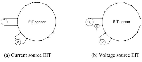
Electrical Impedance Tomography (EIT) was initially invented for medical imaging applications [9-10].

The alternating current source was applied to drive the electrodes, because the magnitude of current

injected into to human body can be controlled within the safety limit. Later, the applications of EIT

technique were utilized for industrial process measurement, but the majority of EIT systems still kept

current as excitation source and sensed voltages as shown in Figure 2 (a). The EIT with current source has

following disadvantages. When aqueous continuous phase is not very conductive, for example distilled

water, response voltages on the sensing electrodes could exceed the maximum input range of the analogue

voltage signal cannot reflect any change of two phase flow. When continuous phase is highly conductive

like sea water, the equivalent mutual impedance is in the order of ohm, only using large current drive

(hundreds mA) can increase the magnitude of response voltage on the electrodes for measurement.

However, it is difficult to design a current source having more than 75mA output in the typical EIT

frequency range 1kHz-1MHz. Moreover, the output of current source does not maintain constant while

the load varies. In SPICE simulation of an EIT’s current source [6], the load impedance is swept from 5

to 1255 and the output amplitude of the current source has 5.93% decrease, which brings in additional error for EIT measurement if this defect of current source is not taken into account. These limitations of

current source restrict the performance and accuracy of EIT.

A recently developed EIT system [11] applies voltage to electrodes as excitation source. The output

current of the voltage source and voltages across electrodes are monitored simultaneously to calculate

mutual impedance (Z=V/I) in the voltage source EIT, which is the variable of the image reconstruction

algorithm in section 3 rather than the voltage values in the current source EIT system. Figure 2 (a) and (b)

illustrate two structures of EIT. The mechanism of the voltage source EIT overcomes the limit of current

source associated with the conventional EIT systems.

V

EIT sensor I

V I

EIT sensor

(a) Current source EIT (b) Voltage source EIT

Figure 2. Schematic of EIT measurement

2. CAPABILITY OF MAXWELL RELATIONSHIP FOR FULL VOID FRACTION

In EIT, by solving the inverse problem, the tomographic image showing the electrical conductivity

contrast is reconstructed using N mutual impedance data acquired from all the impedance projections to

visualise the distribution of dispersed phase. A conductivity image consists of M square pixels, which are

316 in authors’ case. More information can be deduced from the conductivity image, for instance, the

local and overall void fraction of the dispersed phase. Different correlations were proposed to convert

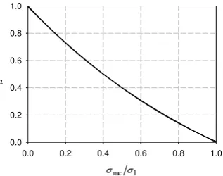
The Maxwell relationship [13] formulated in equation (1) is mostly used to derive void fraction from

conductivity.

_{2( )}

2 2 2 1 1 2 1 2 2 1                     mc mc mc mc

where 1 is the conductivity of aqueous continuous phase (water), 2 is the conductivity of dispersed

phase (air or oil), mc is the mixture conductivity obtained from EIT and is local void fraction. , 1, 2

and mc arethe vectors with M elements (M=316 in authors’ case) and each element represents the value in

the local area. If dispersed phase is non-conductive, 2 is assumed to be zero and equation (1) is simplified

as: 1 1 2 2 2         mc mc (2)

Rearrange equation (2), the conductivity ratio mc/ 1 becomes the only variable in equation (3) to

determine the void fraction .

1 1 2 2 2     mc mc   

Equation (3) describes the correlation between two vectors. Each individual element of mc/ 1 and will

satisfy the equation too. In air-water or oil-water two phase flows, the mixture conductivity mc must be in

the range of 0 ≤ mc≤ 1. Then, the conductivity ratio mc/ 1 is 0≤ mc/ 1≤1. On one extreme condition, if

the flow pipeline is full of non-conductive dispersed phase, like air or oil, the mixture conductivity mc

becomes 0 and the conductivity ratio mc/ 1 equals to 0. Therefore, in equation (3) is 1. On another

extreme condition, if the flow pipeline is full of aqueous continuous phase, like water, the mixture

conductivity mc is identical with 1, and the conductivity ratio mc/ 1 becomes 1 and in equation (3) is 0,

which means no dispersed phase presents in the mixture at all. For simplicity, Figure 3 graphically

illustrates the correlation between one element of mc/ 1 and the corresponding . Although mc/ 1 and

do not follow linear relationship with respect to equation (3), the void fraction obtained from equation (3)

falls in the range of 0~1, provided that the conductivity ratio mc/ 1 is known. Two algorithms of

calculating mc/ 1 will be compared in next section.

(1)

0.0 0.2 0.4 0.6 0.8 1.0 0.0

0.2 0.4 0.6 0.8 1.0

1



mc

Figure 3. Relationship between the conductivity ratio mc/ 1 and void fraction

3. IMAGE RECONSTRUCTION ALGORITHM

The process of image reconstruction in EIT is to determine the unknown electrical conductivity based on

the known voltage on the electrodes or mutual impedance in our case. In fact, this is a nonlinear process in

electrical tomography; moreover, the N number of the known mutual impedance is much less than the M

number of unknown conductivity. These challenges make finding the precise unknown electrical

conductivity very difficult. There are many image reconstruction algorithms were developed for EIT [14].

They are separated into two categories, qualitative non-iterative algorithms and quantitative iterative

algorithms. Non-iterative algorithms only involve the multiplication between a matrix and a vector.

Although the images reconstructed from these algorithms are not sharp and clear, their computational

speed is so fast that only non-iterative algorithm can be implemented in EIT to conduct on-line

measurement and control for multiphase flow. Iterative algorithms can deliver relatively better images but

in the cost of longer computational time. These algorithms are suitable for the applications requiring

higher quality to the off-line images for instance medical imaging. Since the targeted application in this

paper is dynamic multiphase flow measurement, only non-iterative algorithms are discussed.

Due to the addition of dispersed phase, the change of mutual impedance Z and the change of

conductivity in the medium are respectively defined as

ZZmcZ₁ (4)

where Z1 is the baseline mutual impedance measured from EIT sensor containing only single continuous

phase with conductivity 1. Zmc is mutual impedance after two phase mixture presents and conductivity is

altered to mc.

Computing the change of mutual impedance Z from the known conductivity change is a forward

process and described as

) (



Z F

(6)

where F is a forward operator and can be solved by the finite element methods.

An alternative approach to solve equation (6) is to use Taylor series in equation (7)

( ) (( )2)

   

  

Z F (7)

Based on the condition of  ₁, high order terms O(( )2) is omitted and equation (7) is linearized

into equation (8). If the condition of  ₁cannot be satisfied, large numerical error will occur.

  '

S

Z (8)

where ' _{1 1}

)

( 

  F

S is defined as sensitivity matrix and 1 is the baseline conductivity. The minus sign

of equation (8) indicates conductivity and mutual impedance have opposite change direction. The

normalised form of equation (7) is expressed as:

1 1        S Z

Z ₍₉₎

Where S is the normalised sensitivity matrix and formulated as equation (10), i is the location of

excitation-measurement projection, k is the pixel number and M is the total number of image pixels.



 _M

k ik j i s s S 1 , ' , ' (10)

To find the relative conductivity changes / 1 from the relative mutual impedance changes Z/Z1 is the

inverse process of equation (9), which still remains a challenge to find the exact inverse matrix of S in EIT

imaging. Kotre [15] developed the Sensitivity Back-Projection (SBP) algorithm based on the Linear

Back-Projection (LBP) principle, where inverse S-1 is approximated to its transpose matrix ST as shown in

equation (11), because S is not a square matrix. This approximation gives the best fit from the least square

1 1 1 1 Z Z S Z Z

S   T

   _   (11)

Substitute equation (4) and (5) into equation (11), the first method of calculating mc/ 1 is illustrated in

equation (12). 1 1 1 1 Z Z Z ST mc

mc    



 ₍₁₂₎

In equation (13), the modified Sensitivity Back-Projection (MSBP) based on the nonlinear approximation

[17] was proposed as an alternative approach to gain mc/ 1.

1 1 1 Z Z ST mc

mc     (13)

Substitute equation (12) and (13) into equation (3) individually, the ultimate correlations between void

fraction and mutual impedance ratio Zmc/Z1 are expressed in equation (14) and (15).

T mc T T mc T S Z Z S S Z Z S       1 1 3 2 2  (14) _{2 1} 2 1 1      Z Z S Z Z S mc T mc T  (15)

in equation (14) and (15) contains M elements representing the void fraction of dispersed phase in local

image pixel area. The overall cross-sectional void fraction A is the average of M element in .

M

A

M

i i



 1

(16)

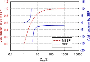
In order to visualise the correlation between mean void fraction A and mutual impedance ratio Zmc/Z1 in an

ideal and simply perspective, it is assumed that the vector Zmc/Z1 has N elements with the same value. Two

correlations are plotted in Figure 4. Thelogarithm scale is applied for the x-axis Zmc/Z1 to demonstrate a

wider Zmc/Z1 range. The red dashed curve in Figure 5 shows that in MSBP algorithm, the mean void

fraction does not exceed the range of 0~1 with respect to the variation of Zmc/Z1 from 1 to 1000, despite

the correlation is not in linear relationship. On the contrary, the blue solid curveindicates the correlation

range of 3.95~4.00. Figure 5 suggests the SBP algorithm only can present meaningful and valid results

when Zmc/Z1 is less than 2. Other values of Zmc/Z1 result in the mean void fraction beyond the range of 0~1.

Zmc/Z1

0.1 1 10 100 1000 10000

Vo id fractio n   by MSB P 0.0 0.2 0.4 0.6 0.8 1.0 1.2 Vo id fractio n   by SB P -20 -15 -10 -5 0 5 10 15 MSBP SBP

Figure 4. Correlation of mutual impedance ratio Zmc/Z1 and mean void fraction A

To compare two correlations only in the valid range of SBP algorithm, Figure 4 is re-plotted into Figure 5

only when the conductivity ratio Zmc/Z1 is from1 to 2.2. Both correlations output 0 void fraction when

Zmc/Z1 equals to 1, however, the divergence of SBP and MSBP is dramatically intensified once Zmc/Z1 is

larger than 1.6. It is concluded that the MSBP algorithm is a better correlation than the SBP algorithm. In

the next section, only MSBP algorithm is applied for the computation of void fraction.

0.8 1.0 1.2 1.4 1.6 1.8 2.0 2.2 2.4

Vo id fractio n   by MSB P 0.0 0.2 0.4 0.6 0.8 Vo id fractio n 

by SB

P 0.0 0.2 0.4 0.6 0.8 1.0 1.2 1.4 MSBP SBP

Figure 5. Valid Zmc/Z1 range of SBP in Figure 4

4. EXPERIMENTS

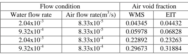
The experiment was conducted out in a Perspex flow loop with 0.058 m inner diameter of and 3.0 m

vertical section. The detailed schematic of the experimental flow loop is referred in literature [7]. The

mean air void fractions obtained from the voltage source EIT system [11] and Wire-mesh sensor (WMS)

are compared in Table 1. At the flow conditions with air void fraction range less than 0.30; the void

fraction delivered by EIT is close to that of WMS.

Table 1. Air void fraction measured by WMS and EIT

Flow condition Air void fraction

Water flow rate Air flow rate(m3/s) WMS EIT

2.04x10-3 8.33x10-5 0.04345 0.04432

9.32x10-4 8.33x10-5 0.05978 0.06828

2.04x10-3 8.33x10-4 0.22892 0.23263

9.32x10-4 8.33x10-4 0.29673 0.31884

4.2 Static EIT Vessel Experiment: Packed Particles

Due to the capability of the existing laboratory flow loop, it is difficult to create a flow regime with air

void fraction larger than 0.5. In order to create two phase mixture having larger void fractions, a number

of static setups with the packed particles were used. A 50.8mm diameter static EIT vessel was filled up

with 305.0mL tap water for the reference baseline taken by EIT. Later, non-conductive yellow spherical

particles with 6.00mm diameter were gradually poured into the vessel. At the same time, water was

carefully removed and collected from the vessel, until the mixture reaches the same water level as the

reference setup, to keep the total volume of mixture the same as 305.0mL. The volume of water repelled

by particle was 175.0mL. As shown in Figure 6(a), particles were randomly packed and the mixture was

regarded as homogenous. The true void fraction of particles was calculated as 0.5738 (175.0mL/305.0mL).

The measured void fraction of EIT using equation (15) was 0.5922. Since particles are homogenous

packed, the 2D cross-sectional void fraction measured by EIT can represent the real 3D void fraction

estimated by the volume ratio of particles and water.

To further increase the void fraction, the pervious experiment procedure was repeated. The only

difference was the second type of non-conductive blue particles with 0.72mm diameter were carefully

poured into the vessel as well when the 6.00mm particles were poured into the vessel as shown in Figure

6 (b). These fine purple particles filled in the space between the larger yellow particles, so a larger void

fraction was expected. At this time 222.5mL tap water was repelled. The actual void fraction of particles

(a) (b)

Figure 6. Spherical non-conductive particle randomly packed in the static EIT vessel

(a) 6.00mm (b) 6.00mm and 0.72mm.

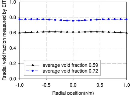
The radial void fraction profiles of two static experiments are demonstrated in Figure 7. Both black and

blue curves exhibit the uniform particle distribution and void fraction cross the centre to the boundary of

the tube. Because the particles are scattered into the tube manually, it might cause the minor fluctuation

on the void fraction profiles.

Radial position(r/m)

-1.0 -0.5 0.0 0.5 1.0

Rradia

l v

oid fract

ion measured by E

IT

0.0 0.2 0.4 0.6 0.8 1.0

average void fraction 0.59 average void fraction 0.72

Figure 7. Radial void fraction profile

4.3 Static EIT Vessel Experiment: Full and Empty

Two extreme conditions, void fraction 0 and 1, is tested in this experiment. When the vessel was full of

tap water in Figure 8(a), the void fraction shown from the EIT was 0.0006. Later, tap water was drained

(a) (b)

Figure 8. Full (a) and empty (b) EIT vessel.

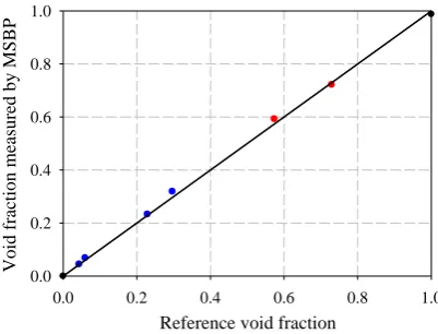
The void fractions of dispersed phase from all pervious experiments are plotted against reference void

fractions in Figure 9. The first and last black points are referred to the full and empty EIT sensor

respectively. Four blue points are from air-water flow measurement and referred to the Wire-mesh sensor

in the experiment 4.1. Two red points are referred to the volumetric ratio between particles and total

mixture in the experiments 4.2. A strong linear relationship between the measured void fraction by EIT

and reference void fraction presented in Figure 11.

Reference void fraction

0.0 0.2 0.4 0.6 0.8 1.0

Void fract

ion

measur

ed by MSBP

0.0 0.2 0.4 0.6 0.8 1.0

Figure 9. Void fractions presented by EIT from different experiments vs. reference void fraction.

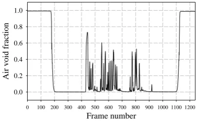
A qualitative dynamic air-water flow experiment was carried out on a 50.8mm water column mounted

with EIT sensors. The column was empty up to frame number 172. The EIT system showed 0.9918 air

void fraction. Tap water was perfused from the bottom of the column. From frame number 215 to 428,

there was full water in the column. The air void fraction dropped down to 0.0006. Then, air was freely

blown from the bottom into the water column until frame 922. The variation of the air void fraction was

recorded by the EIT system. From frame 923 to 1101, there was no air injection and the column remained

water only condition. Finally, water was drained out and the column was empty from frame 1129. Figure

10 shows the dynamic change of the air void fraction during whole process. Future work will involve

verifying the air void fraction through entire void fraction range using other sensing modalities,

particularly for the period of frame number 428 to 922. The author infers that the measurement accuracy

of the voltage source EIT system and MSBP algorithm depends on the flow regime. Homogeneous and

quasi-homogenous flow regime will be the ideal application scenario. If EIT electrodes lose electric

contact with the continuous phase, for instance horizontal stratified flow, the measurement error still

remains a challenge.

Frame number

0 100 200 300 400 500 600 700 800 900 1000 1100 1200

Air void fraction

0.0 0.2 0.4 0.6 0.8 1.0

Figure 10. Dynamic air void fraction recorded by EIT.

5. CONCLUSIONS

The conventional Electrical Impedance Tomography (EIT) with current source tends to underestimate the

void fraction of dispersed phase in two phase flow measurement when it is larger than 0.25. The EIT

system with the voltage source simultaneously measures voltage and current then calculates the mutual

impedance of two phase flow, which overcomes the limit of the conventional current source EIT. The

Maxwell relationship has the capability to represent the correlation between relative conductivity change

and void fraction in the full 0 to 1 range. The Sensitivity Back-Projection (SBP) algorithm works only

Modified Sensitivity Back-Projection (MSBP) algorithm is a better conversion from impedance to

conductivity. The performance of the voltage source EIT system over a full void fraction range is

evaluated. The experimental results demonstrate the full void fraction range of two phase flow can be

managed by the EIT system with voltage source.

REFERENCES

1. A. Shaikh, M. Al-Dahhan, “Characterization of the hydrodynamic flow regime in bubble columns via computed

tomography”, Flow Measurement and Instrumentation, Volume 16, Issues 2–3, April–June 2005, Pages 91-98 2. L. Szalinski, L.A. Abdulkareem, M.J. Da Silva, S. Thiele, M. Beyer, D. Lucas, V. Hernandez Perez, U. Hampel,

B.J. Azzopardi, Comparative study of gas–oil and gas–water two-phase flow in a vertical pipe, Chemical Engineering Science, Volume 65, Issue 12, 15 June 2010, Pages 3836-3848

3. H. Li, M. Wang, Y-X. Wu and G. Lucas, “Volume flow rate measurement in vertical oil-in-water pipe flow using

electrical impedance tomography and local”, 11th _{Int. Conf. on Multiphase Flow in Industrial Plants, Palermo,}

Italy, 200.8

4. H. Jin, Y. Lian, S. Yang, G. He and Z. Guo, “The parameters measurement of air–water two phase flow using the

electrical resistance tomography (ERT) technique in a bubble column”, Flow Measurement and Instrumentation, Volume 31, June 2013, Pages 55-60.

5. F. Dong, Z.X. Jiang, X.T. Qiao, L.A. Xu, “Application of electrical resistance tomography to two-phase pipe flow

parameters measurement”, Flow Measurement and Instrumentation, Volume 14, Issues 4–5, August–October 2003, Pages. 183-192.

6. M. Wang, Y. Ma, N. Holliday, Y. Dai, R. A. Williams, and G. Lucas, “A High-performance EIT System”, IEEE Sensors Journal 5(2): 2005, Pages. 289-299.

7. C. Olerni, J. Jia and M. Wang, “Measurement of Air Distribution and Void Fraction of an Upward Air-water Flow Using Electrical Resistance Tomography and Wire-mesh Sensor”, Measurement Science and Technology Volume 24, No. 3, 2013.

8. H. -M. Prasser, A. Böttger and J. Zschau, “A New Electrode-mesh Tomograph for Gas–liquid Flows”, Flow Measurement and Instrumentation, Volume 9, Issue 2, 1998, Pages 111-119.

9. Henderson, R.P.; Webster, J.G. (1978). "An Impedance Camera for Spatially Specific Measurements of the Thorax". IEEE Trans. Biomed. Eng. 25 (3): 250–254.

10. Barber, D.C.; Brown, B.H. (1984). "Applied Potential Tomography". J. Phys. E:Sci. Instruments 17 (9): 723– 733.A.

11. J. Jia, M. Wang, H. I. Schlaberg and H. Li, “A Novel Tomographic Sensing System for High Electrically Conductive Multiphase Flow Measurement”, Flow Measurement & Instrumentation. 21, 2010, Pages. 184-190. 12. V.S. Shirhatti, “Characterisation and Visualisation of Particulate Solid-liquid Mixing Using Electrical Resistance

13. J. C. A. Maxwell, “Treatise on Electricity and Magnetism”, Unabridged Third edition, Volume 1, Dover Publications Inc. New York, 1954.

14. W. R. B. Lionheart, “EIT reconstruction algorithms: pitfalls, challenges and recent developments”, Physiol Meas. Volume 25, 2004, pp. 125-142.

15. C. J. Kotre, “EIT Image Reconstruction Using Sensitivity Weighted Filtered Back-projection”, Physiol Meas. Volume 15, 1994, pp. 125–136.

16. T. Dyakowski, F. C. J. Laurent, A. J. Jaworski, “Applications of electrical tomography for gas-solids and liquid-solids flows -a review” Volume 112, Issue 3, 2000, Pages 174-192