Topography discretization techniques for Godunov-type shallow water numerical models: a comparative study

(1)

This is a repository copy of Topography discretization techniques for Godunov-type

shallow water numerical models: a comparative study.

White Rose Research Online URL for this paper:

http://eprints.whiterose.ac.uk/75383/

Article:

Kesserwani, G. (2013) Topography discretization techniques for Godunov-type shallow

water numerical models: a comparative study. Journal of Hydraulic Research , 51 (4). pp.

351-367. ISSN 0022-1686

https://doi.org/10.1080/00221686.2013.796574

[email protected]

Reuse

Unless indicated otherwise, fulltext items are protected by copyright with all rights reserved. The copyright exception in section 29 of the Copyright, Designs and Patents Act 1988 allows the making of a single copy solely for the purpose of non-commercial research or private study within the limits of fair dealing. The publisher or other rights-holder may allow further reproduction and re-use of this version - refer to the White Rose Research Online record for this item. Where records identify the publisher as the copyright holder, users can verify any specific terms of use on the publisher’s website.

Takedown

If you consider content in White Rose Research Online to be in breach of UK law, please notify us by

(2)

Topography discretization techniques for Godunov-type shallow water

numerical models: a comparative study

GEORGES KESSERWANI, Department of Civil and Structural Engineering, University of

Sheffield, Sheffield, UK

Email: [email protected] (Corresponding Author)

ABSTRACT

This paper compares various topography discretization approaches for Godunov-type shallow water numerical models. Many different approaches have emerged popular with Godunov-type water wave models. To date, literature lacks an investigative study distinguishing their pros and the cons, and assessing their reliability relating to issues of practical interest. To address this gap, this work reviews and assesses five standard topography discretization methods that consist of the Upwind, the surface gradient method (SGM), the mathematically balanced set of the SWE (Etta-SWE), the hydrostatic reconstruction technique (Hydr-Rec) and the RKDG2 model. The study further considers mix-mode approaches that incorporate wetting and drying together with the topography discretization. Steady and transient hydraulic tests are employed to measure the performance of the approaches relating to the issues of mesh size, topography’s differentiability, accuracy-order of the numerical scheme, and impact of wetting and drying.

Keywords: Godunov-type schemes, topography discretization methods, comparisons, wetting

and drying, steady and transient flows.

Preprint submitted to the Journal of Hydraulic Research

(3)

1. Introduction

Godunov-type shallow water models are featured with the inherent ability to accommodate

complex flow transitions within the numerical solution (Toro 2001, Guinot 2003, Toro and

García-Navarro 2007). In recent years, they have received applied improvements and have

been incorporated into water industry standard software (Lhomme et al. 2010), and used to

support flood risk management (Néelz and Pender 2010). In this context, applicable

Godunov-type water wave models are at most second-order accurate and require a topography

discretization technique and a wetting and drying condition (see Delis and Kampanis 2009 for

a comprehensive review).

In its simplistic view, a Godunov-type scheme provides a first-order accurate model

that is conceptually based (Godunov 1959). It employs the Finite Volume (FV) framework to

approximate the integral of the flow variables – relative to the shallow water equations (SWE)

cast in a conservative form – as piecewise-constant per local discrete element but with

inter-elemental discontinuities; these discontinuities are combined via the solution of the Riemann

problem to provide a sound approximation to the inter-elemental fluxes (Toro 2001). To

achieve a second-order accurate formulation in a Godunov-type framework, the MUSCL

interpolation approach is often employed (Van Leer 1979), which rests on (extrinsic)

reconstruction of piecewise-linear solutions from the initial local piecewise-constant data.

However, the MUSCL method compromises with larger and non-local calculation stencils.

More recently, with the establishment of the discontinuous Galerkin (DG), a local

second-order (or higher-second-order) accurate Godunov-type formulation may be intrinsically derived from

the conservation laws of the SWE, providing a more sophisticated formulation than the

traditional FV framework (Kesserwani and Liang 2011).

The incorporation of a topography discretization technique with Godunov-type SWE

numerical solvers has been an issue of extreme relevance to their practical development. In

respect of this, various discretization approaches have appeared, over the last two decades,

which are featured with the ability to maintain a correct discrete balance between topography

gradient and the spatial flux. Such a numerical model has been referred to be “well-balanced”

or to satisfy the “C-property” (Bermúdez and Vázquez-Cendón 1994, Greenberg and LeRoux

1996, LeVeque 1998). Among the popular topography discretization approaches, the

sophisticated Upwind approach is the eldest. It was derived by Bermúdez and

Vázquez-Cendón (1994) for a first-order accurate formulation and was then adopted to integrate the

topography within higher-order FV-based Godunov-type models (e.g. García-Navarro and

Vázquez-Cendón 1999, Vulovic and Sopta 2002, Crnjaric-Zic et al. 2004). However, the

Upwind approach is renowned for its complexity in implementation and its limitation to a FV

(4)

topography source term using a cell-centred pointwise approach. It was first reported in Nujic

(1995) for a first-order Godunov-type model, and formally formulated in Zhou et al. (2001)

for a second-order MUSCL scheme. Alternatively, Rogers et al. (2003) approached the SGM

mathematically providing a new well-balanced set for the SWE (referred hereafter to

Etta-SWE) that incorporates the free-surface elevation as a main flow variable, and with which the

topography source term discretizes in pointwise manner. The Etta-SWE approach was further

improved and verified for a MUSCL second-order scheme in the work of Liang and

Borthwick (2009). Another popular approach for constructing well-balanced shallow water

numerical model is the one established by Audusse et al. (2004), which is known as the

hydrostatic reconstruction approach (referred hereafter to Hydr-Rec). The Hydr-Rec method

reconstructs the free-surface elevation – likewise to the SGM – but acts differently to balance

the flux and topography gradients so that to further maintain the positivity of the water depth,

and as such provides the further ability to cope with wetting and drying. The Hydr-Rec

approach has been successfully applied– as a topography discretization technique – to various

high-order Godunov-type models such as WENO-FV and DG methods (Xing and Shu 2006,

Noelle et al. 2007), and further enhanced – as a wetting and drying condition – with both FV

and DG second-order Godunov-type models (Liang 2010, Kesserwani and Liang 2012). As to

the DG method, Xing and Shu (2006) demonstrated theoretically that it is by far the simplest

approach to obtain the well-balanced shallow water numerical model. In light of this,

Kesserwani et al. (2010) devised a second-order Runge-Kutta DG method (RKDG2) that is

effortlessly well-balanced in which the local discrete topography is taken as piecewise-linear

but globally continuous. This topography setting is particular to the RKDG2 framework

which is experienced to be more costly than FV-based Godunov-type model. Unquestionably,

this review is far from being complete and has only focused on the topography discretization

approaches that will serve the purpose of this investigation. Nonetheless, for a more detailed

review including the latest trends on the topic of source terms discretization within

Godunov-type models, the reader is referred, for instance, to the work of George (2008),

LeFloch and

Tanh (2011), and

Murillo and García-Navarro (2010, 2012).

Despite the notable progress in the design of topography discretization techniques,

literature, to date, lacks a study comparing between techniques that are commonly used within

Godunov-type shallow water models. From this perspective, the aim of this article to

diagnostically compare popular topography discretization techniques used within

Godunov-type numerical flow solvers. The selected candidates mainly consists of the five techniques

reviewed above; this study attempts to reveal their pros and cons while addressing questions

that are believed to be of interest to hydraulic modellers, software developers and potential

(5)

(i) To what extent of mesh-resolution and/or problem’s complexity each of the currently

existing topography discretization methods is reliably applicable?

(ii) What is the topography discretization technique that provides the best trade-off between

accuracy, efficiency, robustness for wider range of applications?

The study namely focuses on the Upwind, SGM, Etta-SWE and Hydr-Rec approaches taken,

respectively, with first- and second-order FV formulations, the RKDG2 second-order

formulation and combined approaches incorporating the Hydr-Rec within the different

second-order formulations. Herein, the key ingredient of each of the selected approaches will

be described, and a total of seven approaches will be investigated using various hydraulic test

cases with increasing level of complexity. The performance of each approach will be explored

and discussed in light of the questions (i) and (ii), and relating to effect of wetting and drying.

[image:5.595.93.541.311.646.2]

Finally, findings will be summarized and key-conclusions will be drawn.

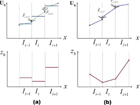
Figure 1.Local discretization of flow and topography data: (a) FV method using

piecewise-constant data, and with which MUSCL interpolation maybe (extrinsically) applied to produce

(6)

2. Depth averagedShallowWaterEquations(SWE)

From the principles of mass and momentum conservation, the 1D mathematical model of the

SWE can be cast in a conservative matrix form:

( )

t x

  

U

F U



S U

(1)

In which (

x

,

t

) are the space-time coordinates. U is the vector of the conserved quantities or

of flow variables, F(U) is the flux vector and S(U) is the vector containing the topography

gradient term:

h

q

 

  

 

U

, 2 2

2

q

q gh

h

 

 

 _ _ _

 

F and

0

x

gh

z





 

_

_







S

(2)

Where g (m2/s) is the constant gravitational acceleration, h (m) is the water depth, q = hu

(m2/s) is the unit-width discharge expressed in terms of the velocity u (m/s). By involving the

Jacobian matrix of the flux with respect to the flow vector (J = ∂F(U)/ ∂U), the system (1) can

be expressed in a quasi-linear form (i.e.

  

_t

U J U

_x



S

). J has two real eigenvalues 1,2 = u

± c (where c  gh is the wave celerity) and has a complete set of independent real

eigenvectors e1,2 = [1, 1,2]T.

3. Godunov typenumericalmethods

A 1D computational domain [xmin; xmax] is subdivided into N uniform cells, via interface

points xmin = x1/2 < x3/2 … < xN+1/2 = xmax, so that a random cell Ii = [xi-1/2; xi+1/2] is centred at xi =

0.5(xi-1/2 + xi+1/2) and of length x = xi+1/2 – xi-1/2. In what follow, the local approximate

solution of the flow variables will be denoted by Uh and, consistently, the local approximation

of topography function will be denoted by zh.

3.1. Finite volume (FV) approximation (first- and second- order)

In an FV framework, a Godunov-type transformation to the conservative form (1) represents

locally the flow variables as piecewise-constant, i.e. | [ ; ]

i

T I  i  hi qi

h

U U , and likewise for

the topography data, i.e. |

i

h I i

z z (see Figure 1a), yielding the semi-discrete formulation

below:



1 / 2 1/ 2



1

| |

i i

I i i I

d

dtUh  x F F Sh (3)

The fluxes, e.g. F_i__{1/ 2} at the interfaces xi+1/2 (shared by adjacent cells Ii and Ii+1), are obtained

(7)





2

1/ 2 1/ 2 1/ 2 1/ 2 1/ 2 1/ 2 1/ 2 1/ 2 1

1 ,

2

Roe p p p

i i i i i i i i

p





            







_





_







F



F



U



e



(4)

that is supported with the following entropy fix (to reinforce capturing of transcritical flows):













1 / 2 1 / 2 1 / 2

*

1 / 2 2

1 / 2 1 / 2 1 / 2

, ,

1 / 2 / 1 / 2 1 / 2 1 / 2

if

/(2 ) / 2 if

and min , max 0, 2

p p p

i i i

p i

p p p p p

i i i

p p p

i ci i i















              _          _  _       (5)

The mean eigenvalues _ip__{1 / 2}, associated eigenvectors e_ip__{1/ 2}, and pth wave strengths



_ip__{1/ 2} can be found via explicit formulae involving the Roe averages of the velocity and celerity,

and the flow variables involved in U_i__{1/ 2} and U_i__{1/ 2} (Roe 1981); where

1/ 2 | (i 1/ 2)

i I xi

 

  h 

U U and

1

1/ 2 |i ( 1/ 2)

i I xi

 

  h 

U U denotes the limits of the approximate

solution at the interface xi+1/2.

To obtain a second-order accurate scheme, these limits are often interpolated using

the MUSCL approach for reconstructing linear solution from the initial

piecewise-local constant approximation (van Leer B, 1979), as shown in Figure 1a:

 

1/ 2 |i 0.5

i I i



  h   h

U U U (6)

 

1

1/ 2 |i 0.5 1

i I i



  h   h

U U U (7)

Where

 

1





1 1

|

i i i i i i I I

i I I

I I   













_



_







h h

h h h

h h

U

(8)





( )r max 0, min(1, )r is the minmod limiter that controls the variation of the slope

components to avoid spurious oscillations that would possibly occur around discontinuities

(Toro 2001). Finally, time-discretization in (3) is achieved using the explicit two-stage

Runge-Kutta (RK) time stepping controlled by the Courant-Friedrich-Lewy (CFL) condition

with a CFL number equal to 0.75.

Alternatively, to obtain a first-order scheme, it suffice to: (a) zero the gradient

terms within (6) and (7), i.e. _{1/ 2} |

i

i I



  h

U U and

1

1/ 2 |i

i I



  h

U U , and (b) use only the first

stage of the RK discretization to lift the solution to the next time level.

3.2. Discontinuous Galerkin (DG) spatial approximation (second-order)

The DG method conceptually extends the local FV interpretation to higher than first-order

accuracy by integrating the Finite Element (FE) notion. The DG method is locally

(8)

DG discretisation (DG2), the sough solution is locally piecewise-linear (i.e. Figure 1b) and is

spanned by two time-evolving FE coefficients, i.e.

|



0

,

1



i

I



i i h

U

U U

. It expands locally as:

 

0 1









,

( )

/ 2

i

i i i

I

x x

x t

t

x

I

x







 



h

U

(9)

The semi-discrete local transformation of the conservative form (1) now produces two spatial

operators for the update of the two local FE coefficients, respectively:

0 0

1 1

( )

0

0 ( )

0

i i i i

t

d

dt

t



 







 





 



U

L

U

L

(10)

Where L0_i and L1_i are the DG2 local discrete representation to the flux and source terms

vectors in (1), which can be manipulated to give (Kesserwani and Liang 2011):





0

1/ 2 1/ 2

1 |

i

i i i I

x

 

 







h

L

F



F



S

(11)



















1 0 1 0 1

1/ 2 1/ 2

0 1 0 1

3 / 3

/ 3

3 / 3

/ 3

6

i i

i i i I i i I i i

I i i I i i

x

 

 















_

_





_





_



h h

L

F

F|

U

F|

U

S |

U

S |

U



(12)

Similar to the second-order version of the FV method, non-oscillatory solution around sharp

gradients is ensured using the minmod limiter. However, the DG method further requires

restricting the slope limiting process to the so-called troubled-slope components, which have

been identified according to the discontinuity detector of Krivodonova et al. (2004). The

fluxes, e.g. at the interface xi+1/2, are evaluated using the also the Roe Riemann solver (4) and

(5), but with a direct involvement of the limits defined by the local piecewise-linear solutions

at xi+1/2 (see Figure 1b). Finally, each of the local coefficients,

0

( )

i t

U and U1i( )t , is advanced

in time using the explicit double-stage RK time discretization, but with a CFL number equal

to 0.3 (Cockburn and Shu 2001).

4. Topographydiscretizationtechniques

This section briefly summarises the key ingredient(s) of the topography discretization models

that are commonly used within the Godunov-type methods presented in Section 3, and will be

compared later in Section 5. The described techniques are all featured by the ability to verify

the discrete balance with the flux gradient for unperturbed steady flows (i.e. satisfy the C

-property or provide a well-balanced scheme).

(9)

The SGM is widely used with FV Godunov-type schemes. It is credited to Zhou et al. (2001)

where a theoretical verification of the C-property is available. Within the scheme (3)-(8) the

operation of the SGM may be summarized as:

1. Reconstruct (h + z = ) limits at interface xi+1/2 from the variable h and the topography z:

1 / 2 ( ) 0.5 ( ) i hi zi i h z





      and



i1 / 2 (hi 1 zi 1) 0.5 i 1(h z)



        .

2. Evaluate the discharge limits at interface xi+1/2:

1/ 2 0.5 ( )

i i i

q_  q  q and q_i__{1 / 2} q_i_₁0.5_i_₁( )q

3. Set a single topography value at interface xi+1/2 defined by the average

1/ 2 ( 1/ 2 1/ 2) / 2

i i i

z_  z_ z_ where z_i__{1/ 2} z_i and z_i__{1/ 2} z_i_₁.

4. Redefine the Riemann states at xi+1/2 according to the averaged topography zi 1/ 2



 :

1 / 2 1 / 2 1 / 2

K K

i i i

h_ 



_ z_ and uiK_{1/ 2} qiK_{1/ 2}/hiK_{1/ 2} (where K   , ). From these, calculate

the flux F_i__{1/ 2} using equation (4), in which U_iK__{1 / 2} [h_iK__{1 / 2},q_iK__{1 / 2}]T

.

5. Repeat steps 1-4 to further evaluate flux at F_i__{1/ 2} interface xi-1/2.

6. Set h (h_i__{1/ 2}h_i__{1/ 2}) / 2 and  _xz (z_i__{1 / 2} z_i__{1 / 2}) /x and use them to evaluate

| i

I h

S in (3).

4.2 Mathematically balanced set of SWE (Etta-SWE)

Initially developed by Rogers et al. (2003) where all derivation details are presented. The

Etta-SWE uses an alternative mathematical form of the SWE, in which the free-surface

elevation becomes the main flow variable, instead of h, so as to mathematically verify the

C-property (Liang and Borthwick 2009). With this change of variables, the conservative

vectorial form (1) is described according to the expressions below:

q



 

  

 

U

, 2

2

( 2 )

2

q

q g

z



      _ _   _   

F and

0

x

g



z





 

_

_







S

(13)

For the scheme (3)-(8) the key-steps of the Etta-SWE may be summarized as:

1. Directly evaluate limits at interface xi+1/2:

1/ 2 0.5 ( )

i i i







    and



ii 1/ 2



i 1 0.5 i 1( )





    

2. Evaluate the discharge limits at interface xi+1/2:

1/ 2 0.5 ( )

i i i

q_  q  q and qi _{1 / 2} qi ₁ 0.5 i ₁( )q



    

3. Repeat the steps 3-5 of the SGM.

4. Set



(



i _{1/ 2}



i_{1/ 2}) / 2

 

 

  and xz (zi _{1 / 2} zi _{1 / 2}) / x

 

 

    , and evaluate |

i

I h

(10)

4.3 Hydrostatic reconstruction approach (Hydr-Rec)

Established by Audusse et al. (2004) and can further account for wet/dry fronts. Within the

scheme (3)-(8), the contribution of the Hydr-Rec may be described as follows:

1. Reconstruct (h + z = ) and evaluate the discharge limits at interface xi+1/2, i.e. do steps 1

and 2 of the SGM.

2. Record velocities at xi+1/2 obtained from the original topography data (i.e. zi 1/ 2 zi



  and

1/ 2 1

i i

z_ z_ ): h_iK__{1 / 2} 



_iK__{1 / 2} z_iK__{1 / 2} and K_{1/ 2} K_{1/ 2}/ K_{1/ 2}

i i i

u_ q_ h_ ; (where K   , ).

3. Topography discretization at interface xi+1/2 with wetting and drying:

a) Re-define numerically z_iK__{1 / 2},* 



_iK__{1 / 2} h_iK__{1 / 2}, (where K   , ).

b) Set a single z-value at xi+1/2 defined by the maximum, i.e.

,* ,* ,*

1/ 2 max( 1/ 2, 1/ 2)

i i i

z_  z_ z_ .

c) Preserve positivity of water at xi+1/2, i.e. h_iK__{1 / 2},*  max 0,



_iK__{1 / 2} z_i_,*_{1 / 2}



, (K   , ).

d) Find discharges incorporating the original velocities, i.e. q_iK__{1 / 2},* h_iK__{1 / 2},* u_iK__{1 / 2}, and

the free-surface elevations at xi+1/2, i.e. 1/ 2,* 1/ 2,* ,*1/ 2

K K

i hi zi





     , associated to the

positivity-preserving water depth the single value of the topography.

e) Ensure that step d) do not possibly cancel the actual water level at a wet/dry front, i.e.

i. Calculate



,*



1 / 2 max 0, 1 / 2 1 / 2

K

i i zi

  

    

  _   _, i.e. after Step 3-b).

ii. Adjust



_iK__{1 / 2},* 



_iK__{1 / 2},*  



_i__{1 / 2} and z_i_,*_{1/ 2} z_i_,*_{1/ 2} 



_i__{1/ 2}.

4. Find the flux F_i__{1/ 2} using h_iK__{1 / 2},* 



_iK__{1 / 2},* z_i_,*_{1 / 2}, and uiK_{1/ 2} qiK_{1/ 2},* /hiK_{1/ 2},* (after step 3).

5. Repeat steps 1-4 to evaluate flux at F_i__{1/ 2} interface xi-1/2.

6. Set h (hi ,*_{1/ 2} hi,*_{1/ 2}) / 2

 

 

  and xz (zi,*_{1 / 2} zi,*_{1 / 2}) / x

 

 

    , and use them to evaluate

| i

I h

S in (3).

4.4 Upwind decomposition (Upwind)

Developed by Bermúdez and Vázquez-Cendón (1994) and is more sophisticated than the

others. The Upwind approach projects, or decomposes, the source terms vector S onto the

characteristic basis using the parameters involved within the Roe flux upwinding (4). The

Upwind discretization is theoretically able to maintain the discrete balance among flux

gradients and the topography gradient; for instance see within Vázquez-Cendón (1999),

García-Navarro and Vázquez-Cendón (2000) for a demonstration of the C-property.

 For the first-order version of scheme (3)-(8), the involvement of the Upwind approach

(11)



1





1



1 / 2 1 / 2 1 / 2 1 / 2 1 / 2 1 / 2

1

| | | | |

2 i

I I Ji Ji i I Ji Ji i

 

     

 

 _    _

h

S   S   S (14)

where,

1

1 1/ 2

1/ 2 1/ 2 2 1/ 2

1/ 2

0

i

i i i

i

J



     







_

_





R



R



and 1/ 2



11/ 2 21/ 2



1 2

1/ 2 1/ 2

1

i i i

i i



    







_{ }

_





R

e



e



_

(15)

and,

  

1 1

1/ 2

2

0

i i i i

h h z z i

x

g   

          

S and

  

1 1

1/ 2

2

0

i i i i

h h z z i

x

g    

          

S (16)

 For a MUSCL second-order scheme (3)-(8), the Upwind approach also applies but

requires a preliminary incorporation of the SGM (i.e. Step 1) to soften the free-surface

gradients prior to the action of the slope-limiter (to ultimately produce reliable water

depth limits at the interfaces)

4.5 Local P1-topography projection within the RKDG2 framework (RKDG2)

In DG methods, the well-balanced property can be genuinely obtained by projecting the

topography function onto the same space of local polynomial approximation (Xing and Shu

2006). For the DG2 setting, the local P1-topography projection reads (Kesserwani et al. 2010):

 

0 1









/ 2

i

h _I i i i

x x

z

x

z

x

I

x



 

 



(17)

1/ 2

0

_{( )}

(

1/ 2

)

(

1/ 2

)

2

i i x i i i x

z x

z

z x dx















(18)

1/ 2

1

_{( )}

(

1/ 2

)

(

1/ 2

)

2

i

x

i i i

i x

x x

z x

z

z x dx

x

   









_

_











(19)

The local approximation of the topography gradient expresses as:





1

0 1 ( 1 / 2) ( 1 / 2)

( )

/ 2 / 2

i

i i i i

x h I x i i

x x z z x z x

z x z z

x x x

 



  

   _  _  

  

  (20)

And the continuity property holds across the entire domain, namely at the interface xi+1/2:

1

0 1 0 1

1 / 2 1 / 2 1 1 1 / 2

( ) | ( ) ( ) |

i i

h i I i i i i i h i I

z x_  z  z  z x_  z_  z_  z x_ _ (21)

The local RKDG2 method taken with the P1-projection of the topography verifies exactly the

C-property (Kesserwani and Liang 2011).

(12)

Among the possible blends, it is strategic to look at mix-mode approaches incorporating the

Hydr-Rec approach owing to its merit for representing wetting and drying. Therefore, the

foreseeable mix-mode approaches for possible study are:

 Etta-SWE & Hydr-Rec. Applies the Hydr-Rec after steps 1 and 2 of the Etta-SWE. It may be used to integrate wetting and drying into a shallow water model based on the

Etta-SWE model (Liang 2010, Wang et al. 2011).

 RKDG2 & Hydr-Rec. Applies the Hydr-Rec with the local RKDG2 solution to the

traditional SWE and the local P1-projection of the topography. However, it requires local

incorporation of the free-surface gradients to stabilize the slope-limiting process (Xing

and Shu 2006, Kesserwani et al. 2010).

 Etta-SWE & RKDG2 & Hydr-Rec. Applies the RKDG2 & Hydr-Rec using the Etta-SWE, which, in effect, implicitly stabilizes the slope-limiting process (Kesserwani and Liang

2012). In terms of performance, this merge is equivalent to the RKDG2 & Hydr-Rec

merge, and hence will not be further investigated in this work.

 Upwind & Hydr-Rec. This merge does not seem to be directly applicable as the Upwind approach requires keeping the original discontinuous topography limits at interfaces,

whereas the Hydr-Rec, contradictorily, needs to impose a single continuous topography

value of these two limits. Therefore, this prospective merge will not be further

[image:12.595.84.511.510.673.2]

investigated in this work.

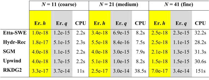
Table 1. Verification of the C-property (i.e. h + z = 6m and q = 0) for the case of the

differentiable topography (22); relative L2-errors (Er.) and CPU times produced by the

second-order Godunov-type models.

N = 11 (coarse) N = 21 (medium) N = 41 (fine)

Er. h Er. q CPU Er. h Er. q CPU Er. h Er. q CPU

Etta-SWE

Hydr-Rec

SGM

Upwind

RKDG2

1.0e-18 1.2e-15 2.2s 3.4e-18 6.9e-15 8.2s 2.5e-18 2.3e-15 32.2s

1.8e-17 5.1e-15 2.3s 5.5e-18 8.4e-16 7.5s 2.5e-18 1.1e-15 28.2s

4.0e-18 1.1e-15 2.2s 4.0e-18 3.0e-15 7.9s 2.1e-18 1.3e-15 31.3s

4.0e-18 1.7e-15 2.2s 5.1e-18 1.0e-15 8.2s 1.5e-18 1.5e-15 30.6s

3.3e-17 3.7e-14 11s 2.5e-17 3.0e-14 38.5s 7.0e-17 3.4e-14 151s

5. Resultsandcomparisons

This section assesses and compares the FV-based topography discretization techniques (i.e.

SGM, Etta-SWE, Hydr-Rec and Upwind), the RKDG2 method and two of the mix-mode

(13)

are implemented with the first-order and the second-order Godunov-type model; whereas the

mix-mode approaches are only considered with the second-order version. Steady analytical

tests are selected to numerically verify the C-property (i.e. h + z = constant and q = 0) and to

benchmark the models’ performance for more complex steady flows (i.e. ∂th = 0 and q =

constant ≠ 0). Unsteady dam-break flows over steps are introduced to elaborate further on the models’ behaviour for conceivable challenging flow scenarios. These particular tests are

mainly distinguished by the property of differentiability for the topography and the flow.

Several mesh sizes are used during the simulations and the relative L2-Errors with respect to

analytical solutions are measured (when applicable) and listed in Tables together CPU

runtime costs.

[image:13.595.91.509.259.495.2]

(a) (b) (c)

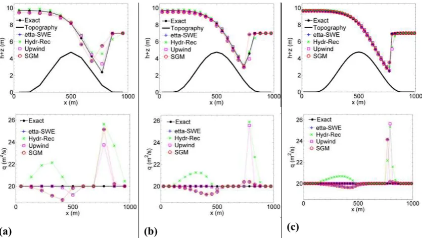
Figure 2. Comparison between the topography discretization models for the first-order FV

schemes; steady flow over differentiable topography: (a) N = 11, (b) N = 21, and (c) N = 41.

5.1 Steady flows over a differentiable topography

Two steady flow sub-cases are considered; the first for verifying numerically the C-property

and the second for assessing the ability to simulate flow with non-zero velocity. The channel

is 1000m long and the topography is featured by the differentiability property and follows a

hump-shape between x = 125m and x = 875m, i.e.

2

125 ( )

4.75

750 x

z x



sin



_







_





(22)

For the first sub-case, the initial conditions are h + z = 6m and q = 0 m2/s with no

external disturbance imposed during the simulations. Therefore the initial state should be

(14)

transmissive or reflective and do not affect the predictions. A series of simulations is carried

out on computational grids with N = 11, 21, 41 cells, respectively, and up to t = 2000s. The

relative L2-errors for the water depths and the discharges produced by the second-order

Godunov-type models are listed in Table 1. The errors are in the range of machine precision

and hence confirm that all the considered topography discretization techniques are able to

balance the numerical flux with topography gradient for a differentiable topography.

[image:14.595.90.510.201.438.2]

(a) (b) (c)

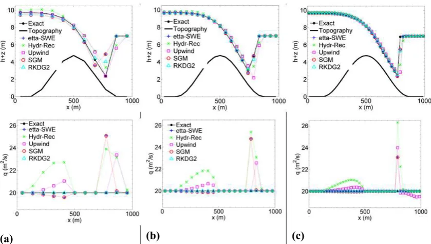
Figure 3. Comparison between the topography discretization models for the second-order

Godunov-type schemes; steady flow over differentiable topography: (a) N = 11, (b) N = 21,

and (c) N = 41.

For the second sub-case, a steady flow with moving water is assumed whereby the

flow undergoes a transcritical flow transition at the middle of the channel and a hydraulic

jump downstream of the hump. A steady inflow boundary condition of 20m2/s is imposed and

the outflow boundary is a water level of 7m. A simulation starts from an initial water height

of 8m, and stops after a relatively long time evolution (i.e. t = 2000s). Sets of simulations are

run, on the same meshes as before, and using the first- and second-order Godunov-type

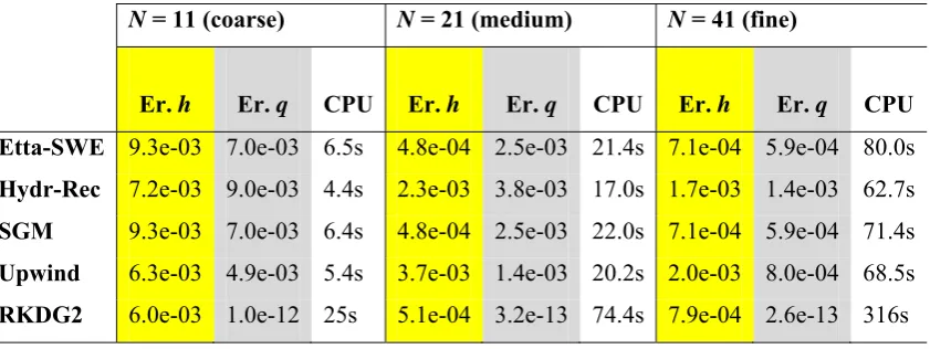
schemes, respectively. Figure 2 and Figure 3 present the respective predictions, where the

numerical depths and discharges realized by the different topography discretization methods

are compared with the analytical depth and discharge. The associated relative L2-errors are

listed in Table 2 and Table 3, respectively.

In the first-order model, as shown in Figure 2 and Table 2, the Upwind approach

outperform the other approaches for all meshes; for the coarsest and medium meshes, its

(15)

Etta-SWE and the SGM are seen to produce similar outcomes (quantitative and qualitative)

with an under-estimating tendency that is observed to reduce with the doubling and

quadrupling in the mesh density. The Hydr-Rec has generally delivered close performance

alike the others but showing a clear trend to over-estimate predictions; its good behaviour is

namely noted in the capture of the hydraulic jump where – together with the Upwind – it

surpasses the Etta-SWE and the SGM for the coarse and medium meshes.

Table 2. L2-error (Er.) for flow variables and CPU times produced using the first-order

scheme at t = 2000s; transcritical flow with shock over a differentiable topography.

Eta-SWE 1.1e-02 7.4 e-03 2.5s 3.2e-03 8.0e-04 7.8s 5.3e-04 8.0e-04 30.7s

Hydr-Rec 8.8e-02 1.0e-02 1.2s 1.2e-03 3.6e-03 5.3s 8.8e-04 1.2e-03 19.4s

SGM 1.1e-02 7.4e-03 1.9s 3.2e-03 8.4e-04 7.1s 5.3e-04 8.0e-04 23s

[image:15.595.91.512.433.591.2]

Upwind 4.2e-03 5.3e-03 1.3s 2.1e-04 9.7e-04 5.2s 8.8e-04 1.1e-03 20.1s

Table 3. L2-error (Er.) for flow variables and CPU times produced by the second-order

schemes at t = 2000s; transcritical flow with shock over a differentiable topography.

Etta-SWE 9.3e-03 7.0e-03 6.5s 4.8e-04 2.5e-03 21.4s 7.1e-04 5.9e-04 80.0s

SGM 9.3e-03 7.0e-03 6.4s 4.8e-04 2.5e-03 22.0s 7.1e-04 5.9e-04 71.4s

RKDG2 6.0e-03 1.0e-12 25s 5.1e-04 3.2e-13 74.4s 7.9e-04 2.6e-13 316s

With the second-order accurate models, as illustrates Figure 3 and Table 3, the Hydr-Rec

and Upwind are detected to comparatively underperform contrasted against the Etta-SWE and

the SGM that are noted to excel with the second-order scheme. For the coarse and medium

meshes, the Etta-SWE and the SGM errors – relative to the second-order scheme – are

observed to be one order-of-magnitude lower than their errors relative to the first-order model

(i.e. Tables 2 vs. Table 3). Moreover, their predictive capability notes drastic improvement

with mesh refinement. Consequently, it is worth commenting that among the FV-based

(16)

appropriate to the second-order MUSCL scheme. The RKDG2 model could mimic the

analytical profiles with an ideal accuracy. Remarkably, its level accuracy is noted to

reasonably match the Etta-SWE and SGM on the fine mesh; however in this setting, the

RKDG2 approach trades-off with an excessive runtime cost (Table 3). Overall, for steady

flow over a differentiable topography, all the FV-based topography discretization approaches

are applicable on reasonably fine meshes. However, these preliminary results suggest giving

preference to Upwind and Hydr-Rec within a first-order scheme and to SGM and Etta-SWE

within the second-order MUSCL scheme. The RKDG2 method, although provides the finest

capture to flow transition, seems to be opportune for very coarse meshes where its runtime are

[image:16.595.86.512.316.734.2]

relatively comparable.

Table 4. Verification of theC-property for a fully wet-domain involving a non-differentiable

topography; relative L2-error (Er.) for flow variables and CPU times.

Eta-SWE 5.9e-18 3.3e-14 3.4s 1.0e-17 5.0e-14 12.3s 1.7e-18 1.3e-14 47.3s

SGM 5.7e-18 1.9e-14 3.5s 7.2e-18 5.3e-14 11.5s 2.0e-18 3.0e-15 44.0s

RKDG2 4.0e-17 1.8e-14 16.9s 2.6e-17 1.2e-14 56.5s 5.8e-17 5.2e-14 210s

(17)

Figure 4. Comparison between the topography discretization approaches for the first-order

FV schemes; steady flow over a non-differentiable topography: (a) N = 11, (b) N = 21, and (c)

N = 41.

[image:17.595.89.512.144.386.2]

(a) _(b) (c)

Figure 5. Comparison between the topography discretization approaches for the second-order

Godunov-type schemes; steady flow over a non-differentiable topography: (a) N = 11, (b) N =

21, and (c) N = 41.

Table 5. L2-error (Er.) for flow variables and CPU times produced by the first-order FV

schemes at t = 2000s; steady smooth flow over a non-differentiable topography.

Eta-SWE 4.1e-04 3.0 e-02 1.4s 2.8e-04 1.4e-03 5.6s 1.1e-04 4.8e-04 21.6s

SGM 4.1e-04 3.0e-03 1.2s 2.8e-04 1.4e-03 4.4s 1.1e-04 4.8e-04 16s

Table 6. L2-error (Er.) for flow variables and CPU times produced by the second-order FV

schemes at t = 2000s; steady smooth flow over a non-differentiable topography.

(18)

SGM 3.6e-04 2.6e-03 3.8s 2.4e-04 1.2e-03 12.6s 8.0e-05 2.8e-04 45.5s

RKDG2 3.6e-04 1.7e-03 16s 1.6e-04 4.0e-04 60s 9.8e-05 2.3e-04 321s

5.2 Steady smooth flows over a non-differentiable topography

Similar aspects, as in Subsection 5.1, are studied herein for steady flows over the same spatial

1D domain but with a non-differentiable topography (e.g. see within Figure 4). Again, in the

first sub-case, the C-property is verified numerically for a quiescent flow conditions, defined

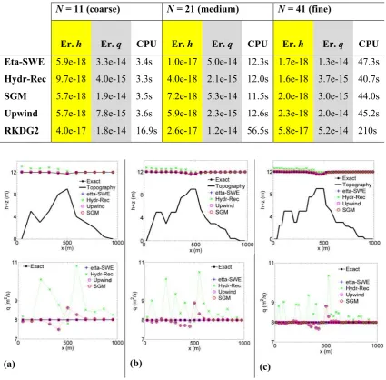
by h + z = 12m and q = 0 m2/s, using the same model configurations, meshes and output time

as in the previous test. As displays Table 3, for all the present topography discretizations have

led to L2-errors that are in the range of round-off. Hence, they all seem to (numerically)

satisfy the C-property irrespective of the mesh size, the accuracy-order of the numerical

scheme and the differentiability property of the topography.

The second sub-case considers a smooth steady subcritical flow where the constant

discharge is 8m2/s and the initial water level is h + z = 12m. Inflow discharge and water level

at the downstream are imposed as physical boundary conditions, which are completed by

transmissive numerical boundary conditions. The same mesh characteristics and output time

as before are used and similar series of simulations are undertaken using the first- and second-

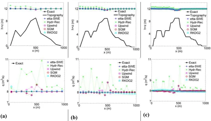
order models, respectively. The predicted depth and discharge produced by the different

topography discretization techniques are compared in Figure 4 and Figure 5, respectively, for

the first- and second-order schemes; Table 5 and Table 6 contain the associated L2-errors that

are measured with respect to the analytical solutions. From these tables, it is noteworthy that

the Upwind approach maintains the top position as being the best match to the first-order

scheme; in this framework, it generates the lowest discharge errors amid any other possible

configuration (including with the second-order schemes) and achieves depth errors with

similar order of magnitude as for the errors produced by the other techniques that performed

best with the second-order schemes (i.e. Tables 5 vs. Table 6). The Etta-SWE and the SGM

maintain the same behaviour noted in the previous test; they delivered similar predictions and,

again, seem to benefit most from the mesh refinement and the increase to second-order

accuracy generating eventually the smallest depth errors overall. The RKDG2 method does

not appear to predict the steady discharge with the same level of accuracy as for the case of

the differentiable topography; yet it provides a close performance to the Upwind, SGM and Etta-SWE approaches with the second-order FV scheme. The Hydr-Rec, in contrast to the

others approaches, fails to supply consistent predictions and hence exposes a clear disability

in handling steady flow over a non-differentiable topography irrespective of the

(19)

Consequently, Upwind, RKDG2, SGM, and Etta-SWE are observed to be reliably applicable

for flow simulation involving non-differentiable topography contrasted with the standard

Hydr-Rec, which its validity is questionable, so far.

[image:19.595.90.511.144.389.2] [image:19.595.92.508.465.702.2]

(a) _{(b) (c)}

Figure 6. C-property verification in a wet/dry domain involving non-differentiable

topography; results produced by the second-order Godunov-type models using a mix-mode

with the Hydr-Rec: (a) N = 11, (b) N = 21, and (c) N = 41.

(a) (b) _(c)

Figure 7. Comparison between the topography discretization approaches reproduced by the

second-order Godunov-type models and in a mix-mode with the Hydr-Rec: (a) N = 11, (b) N

(20)

[image:20.595.87.511.148.248.2]

Table 7. L2-error for flow variables and CPU times at t = 2000s for the smooth over a non-differentiable topography. Mix-mode approaches coupled with the Hydro-Rec within second-order accurate Godunov-type models.

Er. h Er. q CPU Er. h Er. q CPU Er. h Er. q CPU

Etta-SWE 3.6e-03 1.2e-02 3.9s 1.5e-03 4.6e-03 15.0s 7.3e-04 1.7e-03 55.5s

RKDG2 3.6e-04 1.7e-03 18s 1.6e-04 4.0e-04 66s 9.8e-05 2.3e-04 354s

Finally a third sub-case is introduced to further investigate the Hydr-Rec approach

and attempting to gain insight on possible reason(s) for its poor behaviour observed

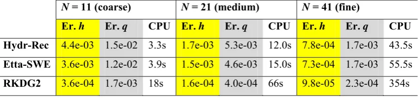
previously. For this purpose, the mix-mode variants Etta-SWE & Hydr-Rec and RKDG2 &

Hydr-Rec (see subsection 4.6) are herein considered –taken together with the second-order

MUSCL scheme. Their C-property ability of the Hydr-Rec variants is re-checked for a

wet/dry initial condition (i.e. h + z = 7m and q = 0m2/s) and they are re-applied to simulate the second sub-case. Figure 6 displays the steady state profiles of the free-surface elevation and

the discharge accomplished by the Hydr-Rec alternatives for the wet/dry C-property test, and

Figure 7 contains their results for the steady moving water over the non-differentiable

topography where their associated L2-Errors are listed in Table 7. As indicate Figure 6, all

Hydr-Rec variants maintain the initial free-surface condition after 2000s and reproduce zero

discharges; hence are able to balance flux and topography gradients for wet/dry domain with

complex topography. On the other hand, when resolving the smooth steady flow over the

non-differentiable topography (wet domain), the Hydr-Rec variants supply dissimilar results. In effect, the incorporation of the Etta-SWE is found to provide insufficient gain in terms of

accuracy, as reflects the depth errors in Table 7 and the discharges prediction displayed in

Figure 7. In contrast, the Hydr-Rec & RKDG2 merge supplies conservative predictions

without showing any signs of potential instability. These findings hence suggest that the

Hydr-Rec and the RKDG2 are supremely compatible for steady flows over non-differentiable

topographies as well as for the unsteady case as it is demonstrated subsections 5.3 and 5.4.

5.3 Transient discontinuous flow over steps

The transient dam-break flow over steps is considered to further explore the topography

discretizations configurations, explored in subsection 5.2, for an unsteady flow over a

(21)

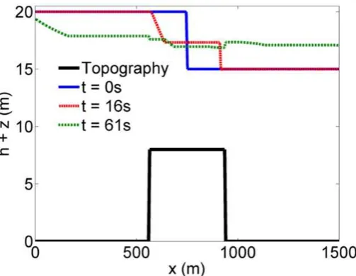
discontinuities and a large abrupt change in the topography level at the step (i.e. from 0m to 8m). The spatial domain is [0; 1500m] and the steps are represented by:

1500 1500

2 8

8 if ( )

0 otherwise

x

z x    

 (23)

The initial condition separates two still water levels as described below,

1500 2

20 ( ) if

( , )

15 ( ) Otherwise

z x

x

h x t

z x







 

_



(24)

Transmissive boundary conditions are used for the upstream and the downstream boundary

cells. Since no analytical solution is available for this test, alternative simulation results

produced by a third order well-balanced RKDG model on a grid with 500 cells are treated as

reference solutions (see Figure 8). Simulations are made on three meshes comprising 100, 200

and 400 cells, respectively. The results at t = 16s and t = 61s, i.e. before and after the

dam-break wave reaches the 8m gap in the bed level, are collected in Figure 9. The upper panel

within Figure 9 presents the zoom-in depth profiles at t = 16s achieved by the Etta-SWE,

SGM, Upwind, Hydr-Rec (with the second-order FV scheme), RKDG2, and the two

mix-mode variants Etta-SWE & Hydr-Rec, and RKDG2 & Hydr-Rec. At t = 16s, all models

delivered fairly similar predictions agreeing closely with the reference solution, namely for

the finest mesh where all the predicted depth profiles seem to overlap. For coarser meshes, the

RKDG2 approach seems also advantageous for the unsteady case as it delivers a more

[image:21.595.172.424.463.658.2]

accurate capture to flow transition than all the FV-based models.

Figure 8. Unsteady dam-break flow profiles over steps at t = 0s, 16s and 61s. Results

produced by the RKDG3 model on a fine grid of 500 cells (Kesserwani and Liang 2011).

At t = 61s, the corresponding zoom-in profiles of the water levels are presented in the

(22)

have closely reproduced the reference solution with the same characteristics as for t = 16s. In this case, however, the anticipated poor behaviour of the FV-based Hydr-Rec variants is seen

to expand leading to predictions that dissociate from the others. This further deterioration in

performance is suspected to occur due to the comparatively high and sharp variation in the

topography gradient at the steps (see next paragraph for the relevant analysis). On the other

hand, the RKDG2 & Hydr-Rec variant is observed to succeed, again, in achieving consistent

predictions in spite of the unsteadiness of flow and the largeness and sharpness of the

topography gradients.

[image:22.595.86.512.240.474.2]

(a) (b) (c)

Figure 9. Magnified numerical depth profiles for the unsteady dam-break flow over steps.

Upper panel: t = 16s, lower panel t = 61s; row (a) N = 100, row (b) N = 200, and row (c) N =

(23)

Figure 10. Action of the Hydr-Rec on the interface topography and relating to the velocity

components (wet case): (a) FV configuration and (b)RKDG2 configuration.

Supported by the present and past numerical experiments, it can be argued that the

Hydr-Rec approach is radically compatible with the RKDG2 framework. In fact, the

underlying reason for this compatibility rests on the continuity property provided by the local

P1-projection of zh within the RKDG2 method, which perfectly helps the Hydr-Rec to avoid

any artificial change in the topography, namely when intertwining with wetting and drying.

To explain this further, Figure 10 demonstrates the local behaviour of the Hydr-Rec at the

second step. As indicate Figure 10(a), the Hydr-Rec particularly records the original velocities

u– and u+ that are associated with original discontinuous values z– and z+, but are required later

for use with the new single topography value z±,* (i.e. obtained via the maximum; step 3-d in

subsection 4.3). Fortunately, the RKDG2 discrete representation to the topography is

continuous (i.e. z+ = z– = z±) and this property provides the Hydr-Rec no other option but to retrieve the original interface topography (i.e. used previously to calculate u– and u+). In

contrast, with the FV method, the Hydr-Rec must cancel the lower value of the topography z+,

to enforce continuity, and hence incompatibly associate its velocity value u+ for use with the

new value z±,*, see Figure 10(a). From the analysis, it appears that the performance of

FV-based Hydr-Rec variants may be exposed to decrease in proportion with an increase in the

height of a topographic step. Supported further by the past numerical experiments, it seems

that the RKDG2 method is, by far, the best complement to the Hydr-Rec to obtain a

second-order accurate and conservative water wave model for flow simulations with uneven

topographies with potential occurrence of wetting and drying.

5.4 Experimental dam-break flow over a step with wetting and drying

Another scenario of a breaking wave over a topographic step is assumed to further examine

the performance of the Hydr-Rec variants when wetting and drying may occur. The 1D

channel configuration is straight with one steep change in the bed level at the middle of

channel, where an imaginary dam is initially assumed. The computational domain is [-10m;

+10m] in which the bed level downstream of the dam is 0.071m and the height of the step is

0.12m. Upstream of the dam, the initial condition of water level is 0.399m. In a first sub-case,

a wet domain is assumed where the initial water level downstream of the dam is 0.075m. In a

second sub-case, the level downstream of the dam is 0m assuming that the wave breaks over a

dry zone. The Hydr-Rec variants are executed on a mesh with 100 cells. Figure 11 shows the

numerical depth profiles reproduced for both sub-cases after 1s and 4s from the dam’s

(24)

In the wet sub-case (Figure 11 – upper panel), the RKDG2 & Hydr-Rec provides the

closest agreement with experimental data providing, eventually at t = 4s, improved capture to

the shock induced by the step and the smooth zone thereafter than the two FV-based

Hydr-Rec variants. The Etta-SWE & Hydr-Hydr-Rec variant does not appear to function better than the

traditional Hydr-Rec, namely at t = 4s in the vicinity of the step where it achieves a poorer

capture to flow. However, in this test, the behaviour of the FV-based Hydr-Rec variants

remains quite satisfactory, contrasted with the observations in the previous test, and this is

likely because of very low height of the step. In the wet/dry sub-case (Figure 11 – lower

panel) all the Hydr-Rec variants are observed to perform globally well suggesting that the

Hydr-Rec approach is functional as a wetting and drying condition within both the FV and the

RKDG2 schemes. Nonetheless, taken as whole, the RKDG2 & Hydr-Rec merge is likely to be

favoured as the best alternative for multipurpose shallow water flow simulations as it does not

particularly risk collapsing in the wet cases in spite of the complexity of the flow and the

non-differentiability of the topography.

[image:24.595.88.512.355.714.2]

(a) _(b)

Figure 11. Experimental dam-break over a step; numerical depth profiles produced by the

second-orderGodunov-type schemes incorporating Hydro-Rec. Upper panel: wet case, lower

(25)

6. Summary,discussionsandconclusions

This work has presented, assessed and compared several topography discretization techniques

relevant to Godunov-type shallow water numerical models. Five different discretization

approaches that satisfy the C-property, i.e. theoretically valid for lake at rest hypotheses, have

been considered and their ability to resolve more complicated flows over topography has been

thoroughly explored. Of these approaches, four are attributed to the FV formulation (up to

second-order via MUSCL interpolation) in which the topography is locally represented as

piecewise-constant with discontinuities at interfaces; whereas the fifth approach is particular

to RKDG2 method (second-order) that locally integrates the topography as piecewise-linear.

The five approaches have been reviewed in their basic form together with alternative

mix-mode forms; they have effectively consisted of:

 The Upwind approach that locally decomposes, i.e. at interfaces, the topography source

term via the projection onto the linearized characteristic basis and thereby discretizes the

topography gradient term in harmony with the local upwinding of the flux.

 The SGM that uses a cell-centred pointwise approximation to the topography gradient. It

first reconstructs free-surface variable at interfaces (i.e. sum of actual depth components

and topography values) and then redefines equivalent Riemann states associated to a

locally-continuous topography at interface (i.e. averaged).

 The Etta-SWE in which the underlying mathematical form of the SWE incorporates the

free-surface component as a main variable. Technically, the Etta-SWE acts on flux and

topography similar to the SGM.

 The Hydr-Rec approach that lies on a depth-positivity-preserving condition to locally

redefine the flux and source term, at interfaces, while satisfying the C-property. It first

maintains the original velocities relative to discontinuous states of the discrete topography

at interfaces. Afterwards, it imposes locally-continuous topography at interfaces (takes

the maximum values) and accordingly redefines new depth components that preserve

positivity. Finally, it employs Riemann states relevant to the positivity-preserving depth

components and incorporating the original velocities to calculate flux, at interfaces, and

discretizes the topography gradient as local pointwise.

 The RKDG2 method that rests on a projection to the topography onto the local basis of

first-order polynomial. The topography projection is continuous, including at the

interfaces, and genuinely integrates the gradient term by a local pointwise manner.

 Mix-mode approaches related to the Hydr-Rec, i.e. Etta-SWE & Hydr-Rec and RKDG2