How does a low-mass cut-off in the stellar IMF affect the evolution of young star clusters?

How does a low-mass cut-off in the stellar IMF affect the evolution

of young star clusters?

M. B. N. Kouwenhoven,

S. P. Goodwin,

R. de Grijs,

M. Rose

and Sungsoo S. Kim

1_{Kavli Institute for Astronomy and Astrophysics, Peking University, Yi He Yuan Lu 5, Hai Dian District, Beijing 100871, China} 2_{Department of Astronomy, Peking University, Yi He Yuan Lu 5, Hai Dian District, Beijing 100871, China}

3_{Department of Physics and Astronomy, The University of Sheffield, Hicks Building, Hounsfield Road, Sheffield S3 7RH, UK} 4_{Harvard–Smithsonian Center for Astrophysics, 60 Garden Street, Cambridge, MA 02138, USA}

5_{Department of Astronomy and Space Science, Kyung Hee University, Yongin-shi, Kyunggi-do 446-701, Republic of Korea}

Accepted 2014 September 8. Received 2014 August 20; in original form 2014 July 22

A B S T R A C T

We investigate how different stellar initial mass functions (IMFs) can affect the mass-loss and survival of star clusters. We find that IMFs with radically different low-mass cut-offs (between 0.1 and 2 M) do not change cluster destruction time-scales as much as might be expected. Unsurprisingly, we find that clusters with more high-mass stars lose relatively more mass through stellar evolution, but the response to this mass-loss is to expand and hence significantly slow their dynamical evolution. We also argue that it is very difficult, if not impossible, to have clusters with different IMFs that are initially ‘the same’, since the mass, radius and relaxation times depend on each other and on the IMF in a complex way. We conclude that changing the IMF to be biased towards more massive stars does speed up mass-loss and dissolution, but that it is not as dramatic as might be thought.

Key words: stars: kinematics and dynamics – stars: low-mass – stars: luminosity function, mass function – open clusters and associations: general.

1 I N T R O D U C T I O N

Star clusters are used as tracers of stellar populations and past star formation in galaxies. A key ingredient of ‘reverse engineering’ an observed population to its initial conditions is knowing how rapidly clusters lose mass and are destroyed (see e.g. Lamers, Gieles & Portegies Zwart2005; de Grijs & Parmentier2007; Chandar, Fall & Whitmore2010; Karl, Fall & Naab2011; Bastian et al.2012; Baumgardt et al.2013).

If a star cluster survives the first few million years, then it will evolve as a result of two-body relaxation, stellar evolution, interac-tion with the Galactic tidal field, close encounters with molecular clouds and the effects of disc and bulge shocking. All these effects contribute to mass-loss and dissolution (e.g. Meylan & Heggie1997; Fukushige & Heggie2000; Heggie & Hut2003; Lamers & Gieles

2006). Numerous studies have investigated the long-term evolution and final dissolution of various types of star clusters under dif-ferent environmental conditions (e.g. Portegies Zwart et al.1998; Baumgardt & Makino 2003; Lamers et al. 2005; Gieles & Baumgardt2008; de Grijs & Anders2012; Shin et al.2013).

One issue that has received relatively little attention recently is the effect of different initial mass functions (IMFs) on the evolution

E-mail:[email protected]

of star clusters. Part of the reason for this lack of interest is the general feeling that the IMF is universal and does not vary among star clusters (e.g. Bastian, Covey & Meyer2010). However, as we shall describe below, there is possibly some evidence for variations, and variations in IMFs are often claimed, so it is worth investigating how star cluster evolution will change given different IMFs.

Previous studies have shown that the long-term survival of star clusters depends on the properties of the low-mass section (a few M) of their IMF. When a deficit of low stellar masses exists, or when the slope of the IMF is too shallow (i.e. when the stellar mass distribution is top-heavy), star clusters will likely disperse within a billion years of their formation (e.g. Chernoff & Shapiro1987; Chernoff & Weinberg1990; Goodwin1997; Smith & Gallagher

2001; Mengel et al.2002). Kim et al. (2006) compared the evolution of clusters with different lower mass cut-offs for the Arches cluster. They find that clusters with the same upper IMF but with two different mass cut-offs (0.1 and 1 M) do not give significantly different luminosity profiles for the Arches cluster at the current age.

Theoretical and observational arguments have been proposed suggesting that the IMF may depend on environment (for a re-view, see Bastian et al. 2010). For example, the upper mass limit of the IMF of a star cluster may depend on the environ-ment in which it forms (e.g. Reddish 1978; Vanbeveren 1982; Weidner & Kroupa 2006), although observational selection

C

effects can complicate the derivation of such a relationship (Parker & Goodwin2007; Maschberger & Clarke2008). Extragalactic stud-ies also suggest that the IMF may be more top- or bottom-heavy in different environments (e.g. Brewer et al.2012; Dabringhausen et al.2012; Dutton, Mendel & Simard2012; Spiniello et al.2012; Zaritsky et al.2012; Barnab`e et al.2013; Bekki2013; Ferreras et al.

2013; Geha et al.2013; Goudfrooij & Kruijssen2013; L¨asker et al.

2013; Smith & Lucey2013; Weidner et al.2013, and numerous others).

Several studies have claimed observational evidence for a top-heavy IMF or a lower mass cut-off in the IMF in young star clus-ters. McCrady, Gilbert & Graham (2003) suggest that MGG-11, a star cluster in the starburst galaxy M82, shows evidence of a top-heavy IMF, with a lack of low-mass stars (M < 1 M). McCrady, Graham & Vacca (2005) also discuss a possible lower mass limit in M82-F. They explain their observations using a top-heavy IMF with a lower mass cut-off at approximately 2 M. Smith & Gallagher (2001) claimed that M82-F has a lower mass cut-off at 2–3 M, but Bastian et al. (2007) show that this may be explained by differential extinction. Another example is NGC 1705-1, where Sternberg (1998) finds that the IMF must be flat or truncated be-lowM<1 M. Mengel et al. (2008) examine young star clusters in NGC 4038/4039 and find that their results can be explained by a significant range in possible IMF slopes or low-mass cut-offs. Greissl (2010), on the other hand, finds no evidence for a low-mass cut-off. Finally, Stolte et al. (2005) find that the present-day mass function in the Arches cluster near the Galactic Centre is truncated below 6–7 M, although Kim et al. (2006) attribute this result to a bump in the IMF around 6–7 M.

In summary, whilst there is no definitive evidence of variations in the IMF with environment (see Bastian et al.2012), there are many claims, and environments, where the observations are unclear. Therefore, the effect of IMF variations on the evolution of star clusters is worth studying, and even if the IMF is truly universal in all environments, this is still an interesting theoretical investigation. In this paper, we carry out numerical simulations of moderately sized star clusters, focusing on the first 200 Myr of their evolu-tion. This article is organized as follows. In Section 2, we describe our method and assumptions. In Section 3, we study how cluster evolution depends on the properties of the IMF, by comparing the evolution of star clusters with varying initial conditions. We dis-cuss the implications of our findings in Section 4 and finally we summarize our conclusions in Section 5.

2 M E T H O D

We simulate ensembles of moderate-mass star clusters (typically a few thousand solar masses) with different IMFs. An important point that we will keep returning to is that it is impossible to create two clusters with different IMFs that are actually ‘the same’ – at least one of the parameters mass, radius or relaxation time will differ between clusters with different IMFs, often significantly.

2.1 Initial conditions

We simulate clusters with typical masses of around 1500 M (al-though this varies from 27 to 17 700 Mfor reasons we will de-scribe below). Clusters are evolved with and without stellar evo-lution to discriminate the dynamical evoevo-lution from that driven by stellar mass loss. We vary the lower mass cut-off in the IMF be-tween 0.1 and 2 M. In order to compare ‘like-with-like’, we run various ensembles in which we keep any two of the cluster mass,

half-mass radius, half-mass relaxation time and the upper end of the IMF, constant.

We use the publicly availableNBODY6 package (Aarseth2003)

for our simulations. Stellar evolution and binary evolution are in-tegrated following the recipes of Eggleton, Tout & Fitchett (1989), Eggleton, Fitchett & Tout (1990), Tout et al. (1997) and Hurley, Pols & Tout (2000).

Each cluster starts as a Plummer sphere in virial equilibrium (following Aarseth, Henon & Wielen1974), and the most massive star allowed in any cluster is 20 M. The fundamental upper mass limit of the IMF may be as high as 300 M(Crowther et al.2010), but what we are effectively doing is ignoring the first few million years of the life of the cluster and starting with a population of clusters that have survived any initial gas expulsion phase, and relaxed into a bound cluster. Therefore, whilst we start our clusters at a formal age of zero, really the starting point for our simulations is an age of 5–10 Myr and any star>20 Mwill have evolved. This avoids complications from what are the true initial conditions from star formation (such as initial substructure; see Allison et al.2010). Also note that 20 Mis the maximum mass one would expect in our canonicalMcl≈1500 Mcluster, either by random sampling

(Parker & Goodwin2007) or from a cluster mass–maximum stellar mass relationship (Weidner & Kroupa2006). It should be noted that, observationally, it is impossible to tell the difference between these two scenarios (Cervi˜no et al.2013). We do not include primordial binaries, nor do we consider primordial mass segregation.

We define a canonical reference cluster with a mass of

Mcl = 1500 M, and a virial radius Rvir = 1 pc, with a

corre-sponding initial projected half-mass radiusRhm=0.59Rvirand an

intrinsic half-mass radius of 0.77Rvir(see e.g. Heggie & Hut2003).

These are typical sizes of young open clusters, although the ob-served spread in radii is large (e.g. Lada & Lada2003; Schilbach et al.2006; Portegies Zwart, McMillan & Gieles2010).

We sample a stellar mass distributionf(M) in the mass range

Mcut ≤M≤ Mmax, whereMcut is a varying low-mass cut-off in

the IMF. We sampleMcutwith values each separated by √

2, i.e. equally in logarithmic space:Mcut≈0.10, 0.14, 0.20, 0.32, 0.50,

0.71, 1.00, 1.41 and 2.00 M. The minimum value ofMcutis near

the hydrogen-burning limit, and the range ofMcutroughly brackets

the values claimed in observational studies. The properties of each of these models are listed in Table1.

We consider both a full Salpeter IMF (e.g. Salpeter1955; Oey

2011) and the Kroupa (2001) IMF. The Salpeter IMF is a power-law

f(M)∝Mαwithα= −2.35. Subsequently, we adopt the more real-istic Kroupa (2001) IMF, a three-part power-law mass distribution, which hasα= −2.3 at the high-mass end. Although the Salpeter IMF is unrealistic down to the hydrogen-burning limit, the effect of a low-mass cut-off is very prominent, and it can therefore be used to illustrate the general behaviour of clusters with a low-mass cut-off in the IMF. The Kroupa (2001) IMF is used to determine how much a low-mass cut-off affects more realistic clusters. For a simple power-law IMF,f(M)∝Mα, the average massM for the Salpeter IMF (withα= −2.35),Mmin=McutandMmax=20 M,

is

M S≈3.86

0.35−M−0.35 cut

0.0175−Mcut−1.35

M. (1)

For the Kroupa (2001) IMF, the average mass can be calculated numerically, and we find that the following expression is a good approximation:

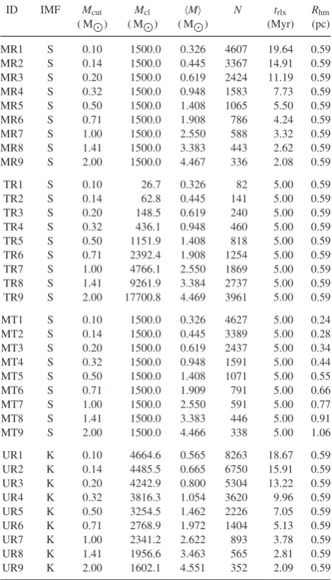
Table 1. Initial conditions of the models used in our analysis. Simulations of each model are carried out with and without stellar evolution. The first column lists the model ID (see Section 2.2). The adopted shape of the IMF (S=Salpeter, K=Kroupa) for each model is listed in the second column. The remaining columns list initial values of the cut-off massMcut, the total cluster massMcl, the average stellar massM, the total number of stars N, the half-mass relaxation timetrlxand finally the half-mass radiusRhm.

ID IMF Mcut Mcl M N trlx Rhm

( M) ( M) ( M) (Myr) (pc)

MR1 S 0.10 1500.0 0.326 4607 19.64 0.59

MR2 S 0.14 1500.0 0.445 3367 14.91 0.59

MR3 S 0.20 1500.0 0.619 2424 11.19 0.59

MR4 S 0.32 1500.0 0.948 1583 7.73 0.59

MR5 S 0.50 1500.0 1.408 1065 5.50 0.59

MR6 S 0.71 1500.0 1.908 786 4.24 0.59

MR7 S 1.00 1500.0 2.550 588 3.32 0.59

MR8 S 1.41 1500.0 3.383 443 2.62 0.59

MR9 S 2.00 1500.0 4.467 336 2.08 0.59

TR1 S 0.10 26.7 0.326 82 5.00 0.59

TR2 S 0.14 62.8 0.445 141 5.00 0.59

TR3 S 0.20 148.5 0.619 240 5.00 0.59

TR4 S 0.32 436.1 0.948 460 5.00 0.59

TR5 S 0.50 1151.9 1.408 818 5.00 0.59

TR6 S 0.71 2392.4 1.908 1254 5.00 0.59

TR7 S 1.00 4766.1 2.550 1869 5.00 0.59

TR8 S 1.41 9261.9 3.384 2737 5.00 0.59

TR9 S 2.00 17700.8 4.469 3961 5.00 0.59

MT1 S 0.10 1500.0 0.326 4627 5.00 0.24

MT2 S 0.14 1500.0 0.445 3389 5.00 0.28

MT3 S 0.20 1500.0 0.619 2437 5.00 0.34

MT4 S 0.32 1500.0 0.948 1591 5.00 0.44

MT5 S 0.50 1500.0 1.408 1071 5.00 0.55

MT6 S 0.71 1500.0 1.909 791 5.00 0.66

MT7 S 1.00 1500.0 2.550 591 5.00 0.77

MT8 S 1.41 1500.0 3.383 446 5.00 0.91

MT9 S 2.00 1500.0 4.466 338 5.00 1.06

UR1 K 0.10 4664.6 0.565 8263 18.67 0.59

UR2 K 0.14 4485.5 0.665 6750 15.91 0.59

UR3 K 0.20 4242.9 0.800 5304 13.22 0.59

UR4 K 0.32 3816.3 1.054 3620 9.96 0.59

UR5 K 0.50 3254.5 1.462 2226 7.05 0.59

UR6 K 0.71 2768.9 1.972 1404 5.13 0.59

UR7 K 1.00 2341.2 2.622 893 3.78 0.59

UR8 K 1.41 1956.6 3.463 565 2.81 0.59

UR9 K 2.00 1602.1 4.551 352 2.09 0.59

We include the external tidal field of the host galaxy, assuming that the cluster is on a circular orbit in the solar neighbourhood. The Jacobi radiusrJof a star cluster of massMclat a Galactocentric

distanceDGcan, to first order, be approximated by

rJ≈DG

Mcl

3MG

1/3

≈6.65

Mcl

1000 M

1/3

pc (3)

(Binney & Tremaine1987), where we adoptMG=5.8×1011M

as the mass of a Milky Way-like galaxy andDG≈8 kpc for the

Galactocentric distance. For star clusters of massMcl≈1500 M

(see Table1), the Jacobi radius is roughlyrJ≈7.6 pc.

As the clusters evolve, stars gradually escape through ejection or through interaction with the Galactic tidal field. Previous work has shown that simple escape criteria such as the binding energy and/or a distance beyond the Jacobi radius are not sufficient, as many stars satisfying these criteria can still spend a significant amount of time

near the cluster and interact with neighbouring stars, or even return to the star cluster (e.g. Terlevich1987; Ross, Mennim & Heggie

1997; Fukushige & Heggie2000). Loosening the escape criteria is a safer approach, but this also has the risk of retaining escaping stars for too long, which is problematic when the process of cluster mass loss is studied. Previous work has indicated that adopting an escaper criterion of twice the Jacobi radius (equation 3) is a practical compromise (e.g. Aarseth1973,2003; Portegies Zwart et al.2001), and this is also the approach we adopt in our study. The consequence of this choice is that we may identify escaping stars slightly too late. For example, when a star formally escapes the star cluster at a distancerfrom the cluster centre at a radial orbit with velocityv, then it will be identified as an escaper at a timet≈ (2rJ−r)/vlater. Our modelled star clusters typically

haverJ≈7.6 pc, and most stars escape with 1–10 km s−1, such that

t<1.5–15 Myr. Although the escape rate and cluster membership are correctly calculated over longer time-scales, caution should be taken when interpreting differences in star cluster membership over shorter time-scales.

The total integration time for each model is 200 Myr, which is substantially longer than the three time-scales that determine the global evolution of the star clusters studied: the stellar evolutionary time-scales, the crossing time and the relaxation time (see Sec-tion 2.2). Depending on the number of member stars in a cluster, we run between tens and thousands of realizations of each model (keep-ingNmultiplied by the number of realizations roughly constant at 1.5×105_{) to reduce statistical fluctuations, which is especially}

important in some cases with very smallN.

2.2 Dynamics and comparisons between clusters

The fundamental process we are interested in is the evolution of the cluster mass with time – i.e. how fast a cluster loses mass, and hence its lifetime. We expect two processes to be important in the evolution of our clusters.

First, and most obviously, stellar evolutionary mass-loss will be important. Stellar evolution will cause stars to lose a significant frac-tion of their mass at the end point of their evolufrac-tion. The time-scale at which stellar evolution becomes important roughly corresponds to 10, 20, 50, 100 and 200 Myr for stars of mass 17.5, 11, 6.8, 4.8 and 3.7 M, respectively: high-mass stars lose more mass, more rapidly than low-mass stars.

So, the greater the fraction of the initial mass of a cluster that is in higher mass stars, the more mass that cluster will lose, and the faster it will evolve.

The effect of stellar evolutionary mass-loss is to cause the cluster to become less massive (obviously), and also to expand. Expansion leads to two effects, one hastens destruction and the other slows it. Expansion causes the crossing time and the relaxation time to increase, so it slows down dynamical evolution and aids survival. But expansion due to mass-loss causes the cluster to fill more of a now smaller tidal radius and eases the loss of stars and hastens destruction. As we shall see, the balance between these effects is important.

In most cases, we take a Salpeter IMF between Mcut and Mmax=20 Mas our IMF. For a Salpeter IMF with a low-mass

cut-off atMcut=0.1 M, the cluster will lose approximately 10 per cent

of its mass in 100 Myr, and approximately 15 per cent by 200 Myr through stellar evolution alone. ForMcut=1 M, the percentages

are 28 and 35 at 100 and 200 Myr, and forMcut=2 M, 42 and

masses of clusters fall byat leastthis amount in 100 and 200 Myr. Any further mass-loss must be due to dynamics.

The other important process in cluster evolution is dynamics: interactions redistribute energy between stars and cause the loss of (preferentially low-mass) stars. This can occur in a violent close encounter, or simply by small perturbations (and the input of tidal energy) causing a star to reach the escape velocity and pass beyond the tidal radius (e.g. Heggie & Hut2003). In addition, scattering events can also result in high-velocity ejections of massive stars (and sometimes even binaries) that have sunk to the centre of the star cluster as a result of mass segregation (see e.g. Gualandris, Portegies Zwart & Eggleton2004), although the vast majority of massive stars evolve before this occurs, and leave the star clusters as stellar remnants (see Section 3).

Dynamical interactions are driven by encounters between stars/stellar systems and the fundamental time-scale for encoun-ters is the crossing time:

tcr=

R

σ, (4)

whereRis the size of the system, andσthe velocity dispersion. The half-mass crossing time in a virialized system is

tcr(half)=

2

G R3

hm

Mcl

, (5)

whereRhmis the half-mass radius,Mclthe total cluster mass andG

the gravitational constant.

Although we do not include primordial binaries, dynamical bina-ries may form through three-body encounters. If the cluster contains a binary system, then that binary can act as an energy sink: en-counters remove energy from the binary, making it ‘harder’ whilst decreasing (making less negative) the potential energy of the rest of the cluster. Close encounters with the binary can also cause ejec-tions. In a star cluster with a single energetically important binary (usually near its centre), the encounter rate with this binary system scales with the crossing time.

Two-body encounters between single stars in the cluster will cause both energy equipartition/mass segregation and evaporation. The global dynamical evolution of star clusters occurs at the time-scale of relaxation. The half-mass relaxation timetrlx for a star

cluster with a Plummer (1911) distribution is

trlx∼

N

8 lnN

tcr(half) (6)

(Heggie & Hut2003), whereNis the number of stars in the cluster (see e.g. Binney & Tremaine1987; Chernoff & Weinberg1990).

Therefore, there are three time-scales that determine the evolution of star clusters:

(i) the stellar evolutionary time-scale (the time-scale on which we lose a significant amount of mass through stellar evolution), which depends onM;

(ii) the crossing time, which depends onRhmandMcl; and

(iii) the relaxation time, which depends on the crossing time (i.e.

RhmandMcl), and also onN(which depends onMclandM ).

Stars also escape when they pass beyond the tidal boundary, which also depends onMcland therefore shrinks as stars evolve and escape

over time. All cluster parameters will evolve with time:MclandN

will always decrease (but not at the same rate) as stars evolve or are ejected, butRhmandM can increase, decrease or stay roughly

the same. Therefore, dynamical time-scales can evolve in complex ways.

2.2.1 Comparing clusters

When studying the effect of varying IMFs on the evolution of star clusters, one would ideally like to only vary one parameter:Mcut,

and henceM . However, as we have seen, changingM changes

N, which changes the relaxation time. Keeping the relaxation time constant then forces us to change other parameters, and so on.

Therefore, we run several different sets of simulations, for each of which we keep the initial conditions of several parameters constant while varyingMcut. The different sets of models, which we refer to

as models MR, TR, MT and UR, respectively, are as follows.

(i)Model MR: the initial total cluster mass and initial half-mass

radius are fixed (Section 3.1).

(ii)Model TR: the initial half-mass relaxation time and initial

half-mass radius are fixed (Section 3.2).

(iii)Model MT: the initial total mass and initial half-mass relax-ation time are fixed (Section 3.3).

(iv)Model UR: the upper part of the IMF and the initial half-mass

radius are fixed (Section 3.4).

The last model, UR, requires some further explanation. In this model, the numbers/masses of stars with masses above 3 Mare kept constant. This is in order to represent clusters that would ‘look’ similar to an observer (for more distant clusters, only the most massive stars can be observed). Therefore, a hypothetical observer looking at any cluster in model UR would see a cluster with the same half-light radius and the same higher mass stellar content. They might not be able to observe that the low-mass cut-off of the IMF varied among these clusters.

Theinitialproperties of each of the models are shown in Table1:

the identifier of the simulations, the initial mass function, the low-mass cut-offMcut, the total massMcl, the average stellar massM,

the number of starsN, the half-mass relaxation timetrlx and the

half-mass radiusRhm.

3 R E S U LT S

A reasonable expectation is that clusters with a highMcut(i.e. a lack

of low-mass stars) will lose mass more rapidly and be destroyed more rapidly that those with a lowMcut.

High-Mcutclusters inevitably lose more mass through stellar

evo-lution than low-Mcut clusters. But the key question of interest is

how this extra (evolutionary) mass-loss changes the rate at which dynamical mass-loss or tidal overflow occurs and so changes the rate at which the cluster is destroyed. In almost all cases we show that the extra evolutionary mass-loss does not have as significant an effect as one might expect.

3.1 IdenticalMclandRhm(model MR)

First, we consider model MR. In this model, we keepMclandRhm

constant. These could be considered the models in which the most basic cluster parameters are kept the same and might be argued to be those in which the clusters are truly ‘the same’. Note that the initial tidal radius is the same for each cluster we consider here.

In the MR models, the initial cluster masses are always

Mcl=1500 M, and the initial half-mass radii areRhm=0.59 pc.

SinceMcutchanges from 0.1 to 2 M,Ndecreases fromN=4607

(M =0.33 M) toN=336 (M =4.5 M). AsMclandRhmare

initially identical for each cluster, so are the crossing times. But as

Ndecreases, the relaxation time falls from 20 Myr (Mcut=0.1 M)

(a)

1 10 100

t (Myr) 0.5

0.6 0.7 0.8 0.9 1.0

N(t)/N(0)

(b)

1 10 100

t (Myr) 0.5

0.6 0.7 0.8 0.9 1.0

M(t)/M(0)

(c)

1 10 100

t (Myr) 1

Rhm

(pc)

Figure 1. Evolution of star clusters with constant initial mass and half-mass radii (model MR) without stellar evolution. (a) Fractional evolution of the number of stars,N. (b) Fractional evolution of the cluster mass,Mcl. (c) Evolution of the half-mass radii,Rhm. In each panel, the darkest curves are for IMF low-mass cut-offs of 0.1 M, becoming lighter as the mass of the low-mass cut-off increases to 2 M.

For model MR, we first consider simulations with no stellar evolution, shown in Fig.1. This paper contains several very similar figures, so it is worth describing them in some detail. Each panel contains several curves with different colours. Darker shades show lower values ofMcutfrom 0.1 M(darkest colour) to 2 M(lightest

colour). In each figure, panel (a) shows the evolution of the relative numbers of stars in each cluster with time. Panel (b) shows the evolution of the relative mass with time and panel (c) shows the evolution of the half-mass radii with time. All results represent the average of an ensemble of simulations.

When we ignore stellar evolution as we do in Fig.1, the evo-lution of clusters will be entirely a result of dynamics. One might expect two-body relaxation to dominate. This would mean that

Mcut=2 Mclusters should ‘evolve’ around 10 times faster than Mcut=0.1 Mclusters (see equation 6). By ‘evolve’ we mean that

the rates at which energy equipartition and ejections occur should be 10 times faster, but this will also be moderated by contraction of the core and expansion of the half-mass radius in response to ejec-tions and evaporation (note that ejecejec-tions can occur with positive energy owing to the tidal truncation).

However, examination of Fig. 1 shows that the evolution of

Mcut=0.1 Mclusters (darkest colour) andMcut=2 Mclusters

(lightest colour) are really quite similar and a significant expansion occurs in all cases. HigherMcutclusters evolveslightlyfaster (the

lightest colour curves are offset), but the difference is not as signif-icant as one might have expected, and certainly not a factor of 10 in the ‘speed’ of the evolution.

The reason for this is that in all of these clusters the dynamics is actually dominated by a massive central binary. The dynami-cal formation of a massive binary system in the centre of a star cluster is very common, and this binary is made of two of the most massive stars in the cluster (see e.g. Aarseth 2003; Heggie & Hut 2003). It acts to heat the cluster, causing the expansion seen in the half-mass radius (Fig.1c). This heating occurs on the time-scale of the crossing time, which is the same in each of these clusters. This shows that dynamics is not as simple as two-body relaxation and can be driven on different time-scales if binaries are present.

The situation we have simulated in Fig. 1is not particularly physical. Apart from the fact that stellar evolution occurs in reality, stellar evolution will be especially important for two other reasons. First, it will cause mass-loss and drive expansion, and secondly, it will also evolve the most massive stars, which are the stars that

tend to be in the dynamically important binary which drives the evolution.

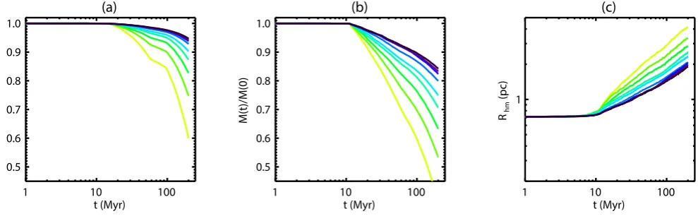
In Fig.2, we show the results of constantMclandRhmclusters withstellar evolution. Here, we have the basic result that one would expect: clusters with a higherMcutlose more mass more rapidly,

expand more rapidly and are destroyed more rapidly. In addition, we show in the bottom panels of Fig.2the results for the individual models in the ensemble of simulations, which give an indication of the spread resulting from stochasticity in the initial conditions and chaos afterwards.

What is particularly interesting is not that clusters with a higher

Mcutlose mass more rapidly (they cannot lose less mass), but that

their mass-loss is not as dramatic as one might have expected. In the very extreme case of a cluster withMcut=2 M, there is still a

surviving cluster after 200 Myr. And the evolutionary sequences of clusters withMcut=0.1–0.5 Mare very similar.

Fig.2(b) and Table2show that this mass-loss is not caused only by stellar evolution. The star clusters withMcut= 0.1 and 2 M

lose 15 and 55 per cent of their mass, respectively, in 200 Myr, only owing to stellar evolution. However, simulations including dynam-ics show that the mass-loss is 20 per cent in theMcut =0.1 M

clusters, and 72 per cent in theMcut=2 Mclusters.

In all cases, the mass-loss is dominated by the mass-loss as a result of stellar evolution, and ejections/tidal overflow only account for about a quarter to a third of the mass-loss.

It seems unexpected that the contribution of dynamical mass-loss is very similar in all cases. Not only do high-Mcutclusters lose more

mass through stellar evolution, but their initial relaxation times are much shorter, which would be expected to drive faster dynamical evolution as well.

However, the rapid and significant mass-loss due to stellar evo-lution causes high-Mcut clusters to expand significantly. This

ex-pansion increases their crossing times, and so significantly reduces their relaxation times, thus ‘slowing’ their dynamical evolution.

In Fig.2(c), we see that the half-mass radii of high-Mcutclusters

(lighter colour curves) expand by factors of several. Indeed, all clusters expand from their initial half-mass radii of 0.6 pc to between 2.4 pc (Mcut =0.1 M) to 5.3 pc (Mcut =2 M). Therefore, all

clusters have significantly longer relaxation times after 200 Myr than their initial values.

Crossing times scale asR3hm/2M− 1/2

cl ; so for theMcut =0.1 M

(a)

1 10 100

t (Myr) 0.5

0.6 0.7 0.8 0.9 1.0

N(t)/N(0)

(b)

1 10 100

t (Myr) 0.5

0.6 0.7 0.8 0.9 1.0

M(t)/M(0)

(c)

1 10 100

t (Myr) 1

Rhm

(pc)

(d)

1 10 100

t (Myr) 0.5

0.6 0.7 0.8 0.9 1.0

N(t)/N(0)

(e)

1 10 100

t (Myr) 0.5

0.6 0.7 0.8 0.9 1.0

M(t)/M(0)

(f)

1 10 100

t (Myr) 1

Rhm

(pc)

Figure 2. As Fig.1, but for the star clusters in model MR with stellar evolution (top panels). The bottom panels show the spread among the individual models in our ensemble of realizations.

by a factor of 50. This acts to help equalize the initial difference in which the initial relaxation times of theMcut=2 Mclusters was

10 times shorter (changingNalso plays a role here to decrease the relaxation times of theMcut =2 Mclusters more, but it is less

significant).

Binary heating can also play a minor role. Fig.2(c) shows that low-Mcut clusters keep expanding significantly, even at late times

when stellar evolutionary mass-loss becomes small (especially after 100 Myr). This expansion is driven by binary heating (although not to the extent that clusters without stellar evolution because of the lower mass of the binaries – compare Figs1c and2c).

An interesting feature is present in the evolution of the number of stars in the clusters in Fig.2(a). The number of stars in the high-Mcut

clusters falls sharply during the first 10–60 Myr, and then slows significantly before declining rapidly again after about 100 Myr. This feature is most prominent in the highestMcutclusters, reducing

in importance as smaller values forMcutare chosen.

The same feature is present in the fractional mass-loss shown in Fig.2(b), but to a much lesser extent (a slight change in the slope of the mass-loss line for highMcut). This feature is the result of

the supernovae of relatively large numbers of stars. The immediate effect of stellar evolutionary mass-loss is to reduce the mass of the cluster, but not the number of stars in the cluster: massive stars change from being 10–20 Mstars into being≈1.4 Mneutron stars. This has two effects.

First, neutron stars are given velocity kicks (for details, see Aarseth2003, andNBODY6), which most often leads to them

be-ing ejected from the cluster – this causes the number of stars to fall fairly rapidly. The production and rapid escape of neutron stars halts around 60 Myr, which explains the kink in Fig.2(a) at this

time. Lower mass stars that do not go supernovae evolve into white dwarfs. These white dwarfs do not get a high-velocity kick, and only escape at around 100 Myr, which explains the second kink in Fig.2(a).

Secondly, the very significant mass-loss caused by stellar evo-lution unbinds a high-velocity tail of stars in the initial velocity distribution. These newly unbound stars take some time to escape the cluster and so are associated with the cluster for some time. This is an effect very similar to that seen in simulations of gas expulsion from star clusters (see especially Bastian & Goodwin2006, who detail the ‘luminosity bump’ caused by slow escapers).

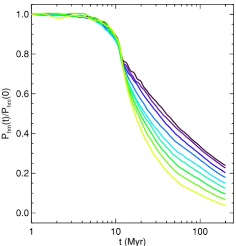
Therefore, we have three effects that cause thenumberof stars to decrease. First, velocity kicks on neutron stars which are responsible for low-mass objects to be lost. This is clearly seen in Fig.3, which shows the cumulative number of neutron stars that have escaped the star clusters over time. In fact, only 1–5 per cent of the stars with masses larger than 10 Mescape before they evolve, while all others experience mass-loss while still being a member of the star cluster. Secondly, the number of stars decreases following the unbinding of high-velocity stars due to the change in the gravita-tional potential from stellar evolutionary mass-loss and the resulting expansion of the star cluster. The potentialPhm(t) at the half-mass

radius, shown in Fig.4, exhibits a strong decrease around 10 Myr, which causes part of the stellar population (which at t= 0 Myr has the same velocity dispersion in all models MR) to escape, and this is most pronounced for the clusters with a highMcut. Thirdly,

the ‘normal’ process of two-body encounters and ejections. All of these processes lead to the loss of relatively low-mass stars in clus-ters with highMcut, leading to a different rate of change in mass-loss

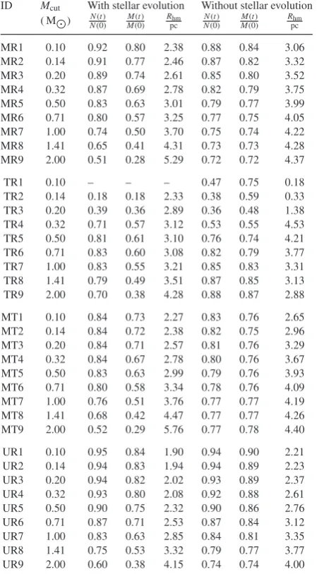
Table 2. Star cluster properties aftert=200 Myr for the initial con-ditions. The first two columns list the model ID and the cut-off mass Mcut. The remaining columns show, both for models with and without stellar evolution, the fraction of the initial number of stars remaining, N(t)/N(0), the fraction of the total initial mass remaining,M(t)/M(0), and the final half-mass radiusRhm. Note that the data for model TR1 (with stellar evolution) are missing, since the majority of these clusters dissolve beforet=200 Myr.

ID Mcut With stellar evolution Without stellar evolution ( M) _NN₍₀₎(t) _MM₍₀₎(t) Rhm

pc N (t)

N(0) M

(t)

M(0) Rpchm

MR1 0.10 0.92 0.80 2.38 0.88 0.84 3.06

MR2 0.14 0.91 0.77 2.46 0.87 0.82 3.32

MR3 0.20 0.89 0.74 2.61 0.85 0.80 3.52

MR4 0.32 0.87 0.69 2.78 0.82 0.79 3.75

MR5 0.50 0.83 0.63 3.01 0.79 0.77 3.99

MR6 0.71 0.80 0.57 3.25 0.77 0.75 4.05

MR7 1.00 0.74 0.50 3.70 0.75 0.74 4.22

MR8 1.41 0.65 0.41 4.31 0.73 0.73 4.28

MR9 2.00 0.51 0.28 5.29 0.72 0.72 4.37

TR1 0.10 – – – 0.47 0.75 0.18

TR2 0.14 0.18 0.18 2.33 0.38 0.59 0.33

TR3 0.20 0.39 0.36 2.89 0.36 0.48 1.38

TR4 0.32 0.71 0.57 3.12 0.53 0.55 4.53

TR5 0.50 0.81 0.61 3.10 0.76 0.74 4.21

TR6 0.71 0.83 0.60 3.08 0.82 0.79 3.77

TR7 1.00 0.83 0.55 3.21 0.85 0.83 3.31

TR8 1.41 0.79 0.49 3.51 0.87 0.85 3.13

TR9 2.00 0.70 0.38 4.28 0.88 0.87 2.88

MT1 0.10 0.84 0.73 2.27 0.83 0.76 2.65

MT2 0.14 0.84 0.72 2.38 0.82 0.75 2.96

MT3 0.20 0.84 0.71 2.57 0.81 0.76 3.29

MT4 0.32 0.84 0.67 2.78 0.80 0.76 3.67

MT5 0.50 0.83 0.63 2.99 0.79 0.76 3.93

MT6 0.71 0.80 0.58 3.34 0.78 0.76 4.09

MT7 1.00 0.76 0.51 3.76 0.77 0.77 4.19

MT8 1.41 0.68 0.42 4.47 0.77 0.77 4.26

MT9 2.00 0.52 0.29 5.76 0.77 0.78 4.40

UR1 0.10 0.95 0.84 1.90 0.94 0.90 2.21

UR2 0.14 0.94 0.83 1.94 0.94 0.89 2.23

UR3 0.20 0.94 0.82 2.02 0.93 0.89 2.37

UR4 0.32 0.93 0.80 2.08 0.92 0.88 2.61

UR5 0.50 0.90 0.75 2.32 0.90 0.86 2.76

UR6 0.71 0.87 0.71 2.53 0.87 0.84 3.12

UR7 1.00 0.83 0.63 2.85 0.84 0.81 3.35

UR8 1.41 0.75 0.53 3.32 0.79 0.77 3.77

UR9 2.00 0.60 0.38 4.15 0.74 0.74 4.00

Therefore, in Fig.2(a), we see significant loss by number during the first 10–60 Myr as a result of the violent early evolution. Subse-quently, there is a slowing of loss by number at 60–100 Myr once all the fast stars have passed over the tidal boundary and are ‘lost’ by the cluster. Then a speeding up of the loss of stars after around 100 Myr as the cluster starts to fill (its now-smaller) tidal radius.

An interesting aside with observational consequences is that the average mass of a star in any cluster remains roughly constant (to within a factor of 2) after around 20 Myr. The most massive stars evolve, but lower mass stars are ejected, causing only a very gradual decline in the average stellar mass in a cluster with time.

ChangingMcutmeans that even though clusters in the MR models

start at the same mass, their luminosities will be very different. Initially, clusters with a highMcutwill bemuchmore luminous than

those with a lowMcut. It might be thought that, as the high-Mcut

1 10 100

t (Myr) 0

10 20 30 40 50

Ncomp,esc

(t)

1 10 100

t (Myr) 0

2 4 6 8 10 12 14

Ncomp,esc

(t)/N(0)

Figure 3. Escaping compact objects for model MR with stellar evolu-tion (cf. Fig.1). The top panel shows thecumulativenumber of compact objectsNcomp, escthat have escaped over time. The bottom panel shows Ncomp, esc/N(0), whereN(0) is the initial number of stars (of all masses) in the star cluster (see Table1). Solid and dashed curves indicate the results for neutron stars and white dwarfs, respectively. All curves are averages for the ensemble of simulations. In each panel, the darkest curves are for IMF low-mass cut-offs of 0.1 M, becoming lighter as the mass of the low-mass cut-off increases to 2 M.

clusters lose so much more of their mass, they will become less luminous.

Let us take our two extreme values ofMcutafter 200 Myr.

Start-ing from initially 1500 M clusters, theMcut =0.1 Mclusters

have become 1200 M clusters with a mean stellar mass of ap-proximately 0.7 M. TheMcut=2 Mclusters have declined in

mass to only∼400 M, but the mean mass of a star is 2 M. So whilst theMcut=0.1 Mclusters have more than 10 times more

stars remaining, the stars that remain in theMcut=2 Mclusters

1 10 100 t (Myr)

0.0 0.2 0.4 0.6 0.8 1.0

Phm

(t)/P

hm

(0)

Figure 4. The evolution of the normalized gravitational potential Phm(t)/Phm(0) at the half-massRhmradius for model MR with stellar evolu-tion. All curves are averages for the ensemble of simulations. In each panel, the darkest curves are for IMF low-mass cut-offs of 0.1 M, becoming lighter as the mass of the low-mass cut-off increases to 2 M.

high-Mcutclusters have lost much more of their mass, they are still

more luminous than the low-Mcutclusters.

In summary, for clusters with the same initial mass and initial (half-mass) radius, those with a higherMcutdo lose more mass. But

this is only really significant in clusters with extremely high values ofMcut(>1 M). For low values ofMcut, the evolution of different

clusters is actually very similar, this is due to expansion slowing dynamical evolution and the equal importance of binary heating in different clusters. This results in a roughly equal importance and rate of dynamical mass-loss in all clusters, regardless ofMcut.

Comparisons of equal-mass and equal-size clusters appear the most sensible, but these would observationally be quite different. If the low-mass component is invisible (e.g. because of distance), then the clusters with a higherMcutwould appear much more luminous

(since more of their mass would be in higher mass stars). Therefore, saying what constitutes ‘the same’ is difficult.

3.2 IdenticaltrlxandRhm(model TR)

Another way of making clusters ‘the same’ is to compare clusters which initially have the same (dynamical) evolutionary time-scale, i.e. the same initial relaxation timetrlx. If the initial relaxation times

of all clusters are the same, then we are considering clusters with the

sameinitialdynamical time-scales – therefore, differences should

be solely due to different stellar evolutionary mass-loss.

Identicaltrlxcan be obtained using equation (6) with a fixedRhm

but varying the number of stars,N, and the total mass of the cluster,

Mcl. BecauseMcldepends on bothNandMcut, this is slightly

non-trivial. In the second block (model TR) of Table1, we can see how bothMclandNmust vary withMcutin order to keep a fixed initial trlx=5 Myr.

The potential problem with these models is clear when we com-pare the differentNneeded in different clusters to keeptrlxconstant

for a constantRhm. WhenMcut=2 M,N=3961, a reasonably

large number. However, whenMcut=0.1 M, we requireN=82

which is so low that we would expect the evolution to be driven by stochastic encounters rather than any statistically ‘smooth’ evolu-tion. Indeed,Mcut=0.1 Msimulations are so stochastic that we

do not illustrate them.

Also note that, by changing the initial cluster mass, we also increase the tidal radius by a factor of 8 betweenMcut=0.1 and

2 M. This allows the clusters with higherMcut to expand more,

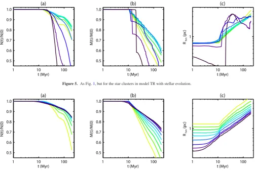
which decreases the time-scale at which they evolve dynamically. The final results of simulations after 200 Myr with stellar evolu-tion are again listed in Table2, and their evolution shown in Fig.5. Interestingly, the evolution withMcutis not simple and falls into two

‘regions’.

In all panels of Fig.5, the low-Mcutclusters (darker colour curves)

show rapid and stochastic evolution due to their smallNand low mass (and therefore small tidal radii). All evolve very rapidly and can form binaries that dominate their evolution (in the models with the smallestMcut, the core radius falls dramatically in a

core-collapse-type event before the star cluster is blown apart). It is difficult to draw any conclusion about evolutionary trends in the low-Mcutcases becauseNis so low. It is also unclear if such low-N

objects constitute a ‘cluster’ under any sensible definition (see e.g. Gieles & Portegies Zwart2011, for a discussion on this topic).

In the cases of highMcut(with reasonableN), we would expect

much less stochastic evolution and this is what we see. Given that each of the clusters has the same initial relaxation time, we might expect stellar evolution to dominate over all else, and this appears to be the case.

Fig.5(c) shows that each of the high-Mcut clusters expands by

approximately the same fraction and at roughly the same rate. This means that higherMcut clusters do not significantly increase their

relaxation times relative to low-Mcut clusters (although the total

mass plays a role).

The expansion is significant enough that in all cases clusters are starting to fill their tidal radii by 100–200 Myr and it is tidal overflow that dominates their mass-loss at late times. This effect is of roughly equal importance in all the high-Nclusters since even though the high-Mcutclusters have lost relatively more mass (thus

reducing their tidal radii), they were initially more massive and so started with larger tidal radii.

To summarize, in the case where we keep the relaxation time and the half-mass radius constant, we get the rather unexpected result that the clusters that survive the longest have intermediateMcut, and

those which are destroyed most rapidly have the lowestMcut.

However, at the low-Mcut end, this is due to low-N stochastic

effects in the dynamics. At the high-Mcut end, this is due to the

significant differences in cluster mass that we need to keep the relaxation times constant, leading to very different tidal boundaries. We would also argue that nobody would sensibly describe two clusters as being ‘the same’ if their masses differ by several orders of magnitude.

3.3 IdenticalMclandtrlx(model MT)

In order to avoid the problems introduced by low-Nstochasticity and large differences in tidal radii in the constanttrlxandRhmmodels

above, we can instead keepMclandtrlx constant and varyNand Rhm. In the third block of Table1(model MT), we can see that to

(a)

1 10 100

t (Myr) 0.5

0.6 0.7 0.8 0.9 1.0

N(t)/N(0)

(b)

1 10 100

t (Myr) 0.5

0.6 0.7 0.8 0.9 1.0

M(t)/M(0)

(c)

1 10 100

t (Myr) 1

Rhm

(pc)

Figure 5. As Fig.1, but for the star clusters in model TR with stellar evolution.

(a)

1 10 100

t (Myr) 0.5

0.6 0.7 0.8 0.9 1.0

N(t)/N(0)

(b)

1 10 100

t (Myr) 0.5

0.6 0.7 0.8 0.9 1.0

M(t)/M(0)

(c)

1 10 100

t (Myr) 1

Rhm

(pc)

Figure 6. As Fig.1, but for the star clusters in model MT with stellar evolution. Rhm=0.24 pc forMcut=0.1 M, andN=338 andRhm=1.06 pc

forMcut=2 M. Note that this is the opposite trend inNwithMcut

as previously, now asMcutincreases,Ndecreases.

Here, clusters are not too ‘different’ – their masses are the same, and their radii only differ by a factor of approximately 4, although the number of stars in each cluster can vary by a factor of over 10. Again, we summarize the final states in Table2, and show the evolution of the key cluster parameters in Fig.6.

In Fig.6, we again see the expected trend that clusters with higher

Mcutand in which stellar evolution is more important (lighter colour

curves) lose more mass than low-Mcut clusters. But yet again, the

differences in the evolution of clusters with differentMcutis not as

extreme as one might expect. By 200 Myr, clusters withMcut=0.1

and 1 Mhave only lost between 27 and 49 per cent of their initial mass, respectively – not a great difference for two such different low-mass cut-offs, both about twice that expected from stellar evo-lutionary mass-loss alone (15 and 28 per cent, respectively).

The reason that the differences are not as great as one might expect is that the evolution of the low-Mcut clusters is driven by

binary heating due to a dense initial state. Low-Mcutclusters have

more stars per unit mass, so in order to keeptrlxconstant,Rhmmust be

much smaller. ForMcut=0.1 M,Rhm=0.24 pc initially, compared

to 0.77 pc whenMcut = 1 M. This leads to central densities of

6×104 _{stars pc}−3 _{in theM}

cut =0.1 M clusters (compared to

approximately 50 stars pc−3_{in theM}

cut=2 clusters). As can be seen

in Fig.6(c), theMcut=0.1 Mclusters start expanding immediately

(and before stellar evolution has any effect). This is caused by rapid binary formation and heating.

Therefore, even though all clusters have the same trlx initially,

within just 10 Myr the Mcut = 0.1 M clusters have expanded

by a factor of approximately 4, decreasing their relaxation times and ‘slowing’ their dynamical evolution. The star clusters with

Mcut = 2 M, on the other hand, do not experience any

signifi-cant expansion during the first 10 Myr, and lose relatively fewer stars and less mass during this time than the clusters with smaller

Mcut. Beyond 10 Myr, stellar evolution sets in, driving expansion,

and loss of stars and mass, which is particularly important for the clusters with highMcut such that they overtake those with lower Mcutin terms of mass-loss. By 200 Myr, theMcut=0.1 M

clus-ters have expanded by a factor of 10, compared to a factor of 5 for theMcut= 1 Mclusters (in their case driven mainly by stellar

evolutionary mass-loss).

Thus, even though all these clusters have the same initial relax-ation time-scales, the low-Mcutclusters change so rapidly that this

initial similarity disappears almost immediately. One could stop the low-Mcutclusters evolving so rapidly by increasing their half-mass

radii by a factor of, say, 10. However, the same scaling would have to be applied to the high-Mcutclusters, giving ‘clusters’ of a few

hundred stars with half-mass radii of 10 pc. Even if such a ‘cluster’ were formally bound at formation, tidal forces would soon destroy it.

(a)

1 10 100

t (Myr) 0.5

0.6 0.7 0.8 0.9 1.0

N(t)/N(0)

(b)

1 10 100

t (Myr) 0.5

0.6 0.7 0.8 0.9 1.0

M(t)/M(0)

(c)

1 10 100

t (Myr) 1

Rhm

(pc)

Figure 7. As Fig.1, but for the star clusters in model UR with stellar evolution.

remain so for long because of processes that have nothing to do with stellar evolutionary mass-loss.

3.4 An identical upper IMF (model UR)

Finally, we describe a set of models in which the high-mass stellar content and the half-mass radii of each cluster are the same. By this we mean that there are the same number of stars with masses greater than 3 Min every cluster: such clusters would appear very similar to observers if seen at a significantly large distance that the low-mass population is ‘invisible’.

If the high-mass stellar content is the same, then for highMcut

there will be few other stars in the cluster, but for lowMcutthere will

be a significant low-mass population. We use the Kroupa (2001) IMF in the mass rangeMcut <M<20 Mand changeMcut. In

all cases, we ensure that there are exactly 200 stars with masses 3<M<20 M.

This means that forMcut =2 M the total number of stars is

only 352, and the total mass approximately 1600 M. But for

Mcut=0.1 Mthe total number of stars is 8263, and the total mass

approximately 4700 M. This means that the relaxation times vary from 2 Myr forMcut=2 Mto 19 Myr forMcut=0.1 M. The

properties of these models are listed in Table1. The results of the simulations are shown in Fig.7.

The high-Mcut clusters must lose much more mass via stellar

evolution than the low-Mcut clusters, and they have much shorter

relaxation times, and are less massive and so have smaller tidal radii. Given all of this, one would expect to see much more rapid and significant mass-loss from high-Mcutclusters.

There is a trend to greater mass-loss from higherMcutclusters

(especially in the extreme 2 Mcut-off), but it is probably not as great as one would expect. From previous arguments, one can see why this is the case.

First, low-Mcut clusters evolve ‘faster’ than one would think.

Fig.7(c) shows the rapid expansion of low-Mcutclusters (as we saw

earlier in Fig.6c). This is driven by the high number densities in these clusters causing binary formation and this driving expansion and ejections. Although difficult to see in Figs7(a) and (b), a handful of stars are ejected before 10 Myr for models with smallMcutbut

not for those with largeMcut, and this difference cannot possibly

be due to stellar evolution. The huge expansion of the low-Mcut

clusters decreases their relaxation times, but the binaries formed in the dense phase are efficient at ejecting stars and keep heating the clusters.

Also, the high-Mcutclusters evolve more ‘slowly’ than their initial

relaxation times would lead one to believe because the significant early stellar evolutionary mass-loss drives expansion and signifi-cantly decreases the relaxation times.

4 D I S C U S S I O N

A key evolutionary property of any star cluster is the rate at which it loses mass, and on what time-scale it is destroyed. Only by knowing these things can we start to ‘reverse engineer’ observed clusters and populations of clusters to their initial states.

The evolution of a star cluster is determined by two fundamental physical processes. First, by dynamics: stars will be ejected over the tidal boundary due to internal dynamics or external perturbations. Secondly, by stellar evolution: stars evolve and lose mass, so reduc-ing the mass of the cluster. But as we have seen, stellar evolution causes changes in the radius and energy of the cluster, which change dynamical time-scales, so these processes are not independent.

In this paper, we have investigated the effect of variations in the low-mass cut-off of the IMF on the evolution of clusters. We have simulated clusters in which the low-mass cut-off of the IMF varies between 0.1 Mand 2 M. For most cases, we have used a pure Salpeter power law over all masses which is not a particularly realistic IMF, but serves our purposes allowing for simple tests of the general effects of altering the IMF.

The expectation of what will happen when the IMF is varied (and these were certainly our expectations on starting this project) is that a higherMcutin the IMF will cause clusters to lose more mass more

rapidly and be destroyed much more rapidly. One would expect this as a cluster with a cut-off at 0.1 Mwill lose around 15 per cent of its mass in 200 Myr as a result of stellar evolution alone, while a cluster with a cut-off at 2 Mwill lose around 55 per cent.

A completely unsurprising result is that clusters with higher mass cut-offs in their IMFs lose more mass. This is unavoidable. However, the results we have described above show that changing the IMF has many important, but rather subtle, effects beyond simply altering the total amount of mass lost by stellar evolution and thus speeding destruction.

What is ‘the same’?An important, but subtle, effect of changing

in order to have any two of mass, radius and relaxation time kept constant, the third property must be changed significantly between different cut-offs (sometimes by orders of magnitude). We would argue that it is impossible and unphysical to ever have two clusters with different cut-offs in the IMF that can otherwise be described as ‘the same’. This is true in terms of the physical properties of a cluster (mass, radius, relaxation time). But it also impacts on the observable properties of a cluster such as the colour/luminosity evolution because the mass-to-light ratio evolves in very different ways. We do not consider these observation problems any further in this paper and concentrate on the underlying physical properties.

How does stellar evolution impact dynamical evolution?Stellar

evolution and dynamical evolution cannot be separated from one another. Stellar evolution causes mass-loss from a cluster which alters the mass and energy of the cluster. In responding to this, clusters will expand, which will increase their crossing times, and hence their relaxation times.

Clusters with a high-mass cut-off in their IMF will lose more mass through stellar evolution than those with a low-mass cut-off. Therefore, they will expand more, and reduce their relaxation times more, and hence dynamically evolve more ‘slowly’. The effect of this is to allow clusters with high-mass cut-offs to survive longer than one might think looking at their initial conditions. The interplay of these effects is rather complex since it depends on what two properties of the cluster were initially ‘the same’.

If a cluster initially has a large radius, then greater expansion can push a cluster towards overflowing its tidal limit thus greatly speeding up its destruction. Alternatively, clusters with very small initial radii can evolve significantly before stellar evolution becomes important because of binary formation and heating.

4.1 Future work

This rather idealized work has shown that the effects of changing the IMF on the evolution of star clusters are rather more subtle than one might have thought. Several interesting lines of enquiry could be followed from this work.

Our treatment of the IMF is rather simple, and a more compre-hensive study should consider changes to both low- and high-mass cut-offs as well as to the shape of the IMF.

A dynamical effect that can be very important is heating by bi-naries. In a number of simulations with very high initial central densities (104_–105_{stars pc}−3_{), binaries can form which heat the}

cluster causing expansion and increased ejections (because of the larger cross-section of a binary). Our simulations contain no primor-dial binaries, despite observational evidence that large fraction of stars in the Galactic field (e.g. Raghavan et al.2010), in young asso-ciations (e.g. Kouwenhoven et al.2005,2007), and in star-forming regions (e.g. Connelley, Reipurth & Tokunaga 2008; Chen et al.

2013; Duchˆene & Kraus2013; Reipurth et al.2014) are part of a binary or multiple system. It is therefore interesting and necessary to include them to investigate their effect(s).

We have touched upon the implications to the observed properties of clusters with different cut-offs in their IMFs but this is clearly something of great importance if one believes that the IMF does vary in some environments.

5 C O N C L U S I O N

We have performed simulations of ensembles of clusters character-ized by different mass cut-offs at the bottom of the IMF.

Our main result is that it is impossible to compare the effects of altering the IMF on two clusters that are otherwise ‘the same.’ If the IMF is changed, then this changes the number of stars per unit mass; therefore, only any two (or some complex combination of) mass, radius, and relaxation time can ever be ‘the same’ initially.

As well as not being ‘the same’ initially, different cut-offs in the IMF cause clusters to evolve differently. Clusters with more stellar evolutionary mass-loss will expand more and hence increase their relaxation times and ‘slow’ their dynamical evolution.

In conclusion, the effect of varying the IMF on the evolution of star clusters is rather subtle and complex. Star clusters that contain many more high-mass stars do lose more mass due to stellar evo-lution, but the impact this has on their destruction might not be as great as one might naively expect.

AC K N OW L E D G E M E N T S

We thank the anonymous referee for her/his insightful comments that helped to improve this paper. MBNK was supported by the Peter and Patricia Gruber Foundation through the PPGF fellow-ship, by the Peking University One Hundred Talent Fund (985) programme, by the National Natural Science Foundation of China (grants 11010237, 11050110414, 11173004) and by STFC under grant number PP/D002036/1. This publication was made possible through the support of a grant from the John Templeton Founda-tion and the NaFounda-tional Astronomical Observatories of the Chinese Academy of Sciences. The opinions expressed in this publication are those of the author(s) and do not necessarily reflect the views of the John Templeton Foundation or the National Astronomical Ob-servatories of the Chinese Academy of Sciences. The funds from the John Templeton Foundation were awarded in a grant to The University of Chicago which also managed the programme in con-junction with the National Astronomical Observatories, Chinese Academy of Sciences. RdG acknowledges partial research support through grants 11043006, 11073001 and 11373010 from the Na-tional Natural Science Foundation of China. We thank the British Council for networking funding through a ‘Research Co-operation grant’ between the University of Sheffield and Kyung Hee Uni-versity under the Prime Minister’s Initiative-2 (PMI2) programme. MR acknowledges funding from the Nuffield Foundation for a 2008 Undergraduate Summer Research Bursary, URB/35327, and STFC (grant number ST/G001758/1). SSK’s work was supported by the Mid-career Research Programme (no. 2011-0016898) through the National Research Foundation (NRF) grant funded by the Ministry of Education, Science, and Technology (MEST) of Korea.

R E F E R E N C E S

Aarseth S. J., 1973, Vistas Astron., 15, 13

Aarseth S. J., 2003, Gravitational N-Body Simulations. Cambridge Univ. Press, Cambridge

Aarseth S. J., Henon M., Wielen R., 1974, A&A, 37, 183

Allison R. J., Goodwin S. P., Parker R. J., Portegies Zwart S. F., de Grijs R., 2010, MNRAS, 407, 1098

Barnab`e M., Spiniello C., Koopmans L. V. E., Trager S. C., Czoske O., Treu T., 2013, MNRAS, 436, 253

Bastian N., Goodwin S. P., 2006, MNRAS, 369, L9

Bastian N., Konstantopoulos I., Smith L. J., Trancho G., Westmoquette M. S., Gallagher J. S., 2007, MNRAS, 379, 1333

Bastian N., Covey K. R., Meyer M. R., 2010, ARA&A, 48, 339 Bastian N. et al., 2012, MNRAS, 419, 2606

Baumgardt H., Parmentier G., Anders P., Grebel E. K., 2013, MNRAS, 430, 676

Bekki K., 2013, ApJ, 779, 9

Binney J., Tremaine S., 1987, Galactic Dynamics. Princeton Univ. Press, Princeton, NJ

Brewer B. J. et al., 2012, MNRAS, 422, 3574

Cervi˜no M., Rom´an-Z´u˜niga C., Luridiana V., Bayo A., S´anchez N., P´erez E., 2013, A&A, 553, A31

Chandar R., Fall S. M., Whitmore B. C., 2010, ApJ, 711, 1263 Chen X. et al., 2013, ApJ, 768, 110

Chernoff D. F., Shapiro S. L., 1987, ApJ, 322, 113 Chernoff D. F., Weinberg M. D., 1990, ApJ, 351, 121

Connelley M. S., Reipurth B., Tokunaga A. T., 2008, AJ, 135, 2526 Crowther P. A., Schnurr O., Hirschi R., Yusof N., Parker R. J., Goodwin

S. P., Kassim H. A., 2010, MNRAS, 408, 731

Dabringhausen J., Kroupa P., Pflamm-Altenburg J., Mieske S., 2012, ApJ, 747, 72

de Grijs R., Anders P., 2012, ApJ, 758, L22

de Grijs R., Parmentier G., 2007, Chin. J. Astron. Astrophys., 7, 155 Duchˆene G., Kraus A., 2013, ARA&A, 51, 269

Dutton A. A., Mendel J. T., Simard L., 2012, MNRAS, 422, L33 Eggleton P. P., Tout C. A., Fitchett M. J., 1989, ApJ, 347, 998 Eggleton P. P., Fitchett M. J., Tout C. A., 1990, ApJ, 354, 387

Ferreras I., La Barbera F., de la Rosa I. G., Vazdekis A., de Carvalho R. R., Falc´on-Barroso J., Ricciardelli E., 2013, MNRAS, 429, L15

Fukushige T., Heggie D. C., 2000, MNRAS, 318, 753 Geha M. et al., 2013, ApJ, 771, 29

Gieles M., Baumgardt H., 2008, MNRAS, 389, L28 Gieles M., Portegies Zwart S. F., 2011, MNRAS, 410, L6 Goodwin S. P., 1997, MNRAS, 286, 669

Goudfrooij P., Kruijssen J. M. D., 2013, ApJ, 762, 107 Greissl J. J., 2010, PhD thesis, Univ. Arizona

Gualandris A., Portegies Zwart S., Eggleton P. P., 2004, MNRAS, 350, 615 Heggie D., Hut P., 2003, The Gravitational Million-Body Problem: A Multi-disciplinary Approach to Star Cluster Dynamics. Cambridge Univ. Press, Cambridge

Hurley J. R., Pols O. R., Tout C. A., 2000, MNRAS, 315, 543 Karl S. J., Fall S. M., Naab T., 2011, ApJ, 734, 11

Kim S. S., Figer D. F., Kudritzki R. P., Najarro F., 2006, ApJ, 653, L113 Kouwenhoven M. B. N., Brown A. G. A., Zinnecker H., Kaper L., Portegies

Zwart S. F., 2005, A&A, 430, 137

Kouwenhoven M. B. N., Brown A. G. A., Portegies Zwart S. F., Kaper L., 2007, A&A, 474, 77

Kroupa P., 2001, MNRAS, 322, 231 Lada C. J., Lada E. A., 2003, ARA&A, 41, 57 Lamers H. J. G. L. M., Gieles M., 2006, A&A, 455, L17

Lamers H. J. G. L. M., Gieles M., Portegies Zwart S. F., 2005, A&A, 429, 173

L¨asker R., van den Bosch R. C. E., van de Ven G., Ferreras I., La Barbera F., Vazdekis A., Falc´on-Barroso J., 2013, MNRAS, 434, L31 McCrady N., Gilbert A. M., Graham J. R., 2003, ApJ, 596, 240 McCrady N., Graham J. R., Vacca W. D., 2005, ApJ, 621, 278 Maschberger T., Clarke C. J., 2008, MNRAS, 391, 711

Mengel S., Lehnert M. D., Thatte N., Genzel R., 2002, A&A, 383, 137 Mengel S., Lehnert M. D., Thatte N. A., Vacca W. D., Whitmore B., Chandar

R., 2008, A&A, 489, 1091

Meylan G., Heggie D. C., 1997, A&AR, 8, 1 Oey M. S., 2011, ApJ, 739, L46

Parker R. J., Goodwin S. P., 2007, MNRAS, 380, 1271 Plummer H. C., 1911, MNRAS, 71, 460

Portegies Zwart S. F., Hut P., Makino J., McMillan S. L. W., 1998, A&A, 337, 363

Portegies Zwart S. F., McMillan S. L. W., Hut P., Makino J., 2001, MNRAS, 321, 199

Portegies Zwart S. F., McMillan S. L. W., Gieles M., 2010, ARA&A, 48, 431

Raghavan D. et al., 2010, ApJS, 190, 1

Reddish V. C., 1978, International Series in Natural Philosophy. Pergamon, Oxford

Reipurth B., Clarke C. J., Boss A. P., Goodwin S. P., Rodriguez L. F., Stassun K. G., Tokovinin A., Zinnecker H., 2014, preprint (arXiv:1403.1907) Ross D. J., Mennim A., Heggie D. C., 1997, MNRAS, 284, 811 Salpeter E. E., 1955, ApJ, 121, 161

Schilbach E., Kharchenko N. V., Piskunov A. E., R¨oser S., Scholz R.-D., 2006, A&A, 456, 523

Shin J., Kim S. S., Yoon S.-J., Kim J., 2013, ApJ, 762, 135 Smith L. J., Gallagher J. S., 2001, MNRAS, 326, 1027 Smith R. J., Lucey J. R., 2013, MNRAS, 434, 1964

Spiniello C., Trager S. C., Koopmans L. V. E., Chen Y. P., 2012, ApJ, 753, L32

Sternberg A., 1998, ApJ, 506, 721

Stolte A., Brandner W., Grebel E. K., Lenzen R., Lagrange A.-M., 2005, ApJ, 628, L113

Terlevich E., 1987, MNRAS, 224, 193

Tout C. A., Aarseth S. J., Pols O. R., Eggleton P. P., 1997, MNRAS, 291, 732

Vanbeveren D., 1982, A&A, 115, 65

Weidner C., Kroupa P., 2006, MNRAS, 365, 1333

Weidner C., Kroupa P., Pflamm-Altenburg J., Vazdekis A., 2013, MNRAS, 436, 3309

Zaritsky D., Colucci J. E., Pessev P. M., Bernstein R. A., Chandar R., 2012, ApJ, 761, 93