promoting access to White Rose research papers
White Rose Research Online [email protected]
Universities of Leeds, Sheffield and York
http://eprints.whiterose.ac.uk/
This is an author produced version of a paper published in Regional Environmental Change.
White Rose Research Online URL for this paper:
http://eprints.whiterose.ac.uk/76571/
Paper:
Fleskens, L, Nainggolan, D, Termansen, M, Hubacek, K and Reed, MS (2013) Regional consequences of the way land users respond to future water availability in Murcia, Spain. Regional Environmental Change, 13 (3). 615 – 632.
1
Regional consequences of the way land users respond to future
1water availability in Murcia, Spain
23
Luuk Fleskens1, Doan Nainggolan1, Mette Termansen2, Klaus Hubacek3 and Mark S. Reed4 4
5
1
Sustainability Research Institute, University of Leeds, United Kingdom; 2 University of Aarhus, National
6
Environment Research Institute, Department of Policy Analysis, Frederiksborgvej 399, 4000 Roskilde,
7
Denmark; 3Department of Geography, University of Maryland at College Park, USA; 4Aberdeen Centre for
8
Environmental Sustainability and Centre for Planning & Environmental Management, School of Geosciences,
9
University of Aberdeen, United Kingdom.
10 11
Abstract
12
Agricultural development in the Murcia autonomous region, Spain has led to overexploitation 13
of groundwater resources and climate change will further increase pressures. Policy options 14
to tackle the current unsustainable situation include the development of inter-basin water 15
transfer (IBWT) schemes from wetter regions in the north and the introduction of taxation to 16
further control groundwater abstraction. Under these scenarios farmers with current access to 17
water could face higher water cost, whereas farmers in areas where water was previously not 18
available could see first time availability of water resources. In this paper we combine 19
discrete choice based interviews (DCI) with farmers in the Torrealvilla catchment, in which 20
they indicate how they would adapt their land use under different scenarios, with an input-21
output model to assess the aggregate effects of individual land use decisions on the economy 22
and water consumption of the Murcia region. The paper presents steps taken in the 23
development of an input-output table for Murcia, including disaggregation of the agricultural 24
sector, accounting for sector water use, and consideration of back- and forward linkages. We 25
conclude that appropriate taxation can lead to better water use efficiency, but that this is 26
delicate as relatively small changes in prices of agricultural products can have significant 27
impacts on land use and water consumption. Although new IBWT schemes would enable 28
water to be used more efficiently, they would considerably increase regional water 29
consumption and the regional economy’s dependence on water. As this is not sustainable 30
under future climate change, water saving development pathways need to be explored. 31
32 33
1. Introduction
34 35
Provision of freshwater is one of the most important ecosystem services, which has in many 36
areas of the world been compromised by unsustainable land management practises (MA, 37
2005). Water resources are limited and need to be carefully managed to satisfy and safeguard 38
continuous multiple needs of consumers, the economy and environment. Water scarcity, the 39
temporal or spatial imbalance between available water resources and demand has been, and 40
will increasingly become, a serious concern, exacerbated by overexploitation, environmental 41
degradation, pollution and climate change (Hubacek and Sun, 2005). 42
43
The Spanish Region of Murcia (Figure 1), despite being hot and dry, has witnessed 44
remarkable agricultural development over the last decades. However, its agricultural sector is 45
premised on heavy overexploitation of groundwater resources and reliance on the Tagus– 46
Segura inter-basin water transfer (IBWT) scheme, which was inaugurated in 1979 (Garrido et 47
al., 2006; Grindlay et al., 2011) and is for 56 ± 15% used for irrigation (CREM, 2011) . The 48
region has become known as a major producer of fruits and vegetables. This is reflected in 49
2
regional gross added value against 4.5% and 2.6% at the national level, respectively), but 51
most significantly by the fact that agricultural exports make up 35.4% of Murcia’s total 52
exports (CREM, 2011). The paradoxical issue of the embedded ‘virtual’ water exports from a 53
water-scarce region has drawn attention from many scholars (Ma et al., 2006; Velázquez, 54
2006; Dietzenbacher and Velázquez, 2007; Downward and Taylor, 2007; Guan and Hubacek, 55
2007; Chapagain and Orr, 2009; Zhao et al., 2009). For the past thirty years, regional water 56
demand in the Segura basin has surpassed availability of renewable water resources as a 57
combined effect of increased irrigation (87% of current water demand) and rapid urbanization 58
(7%) (Grindlay et al., 2011). As a result, ironically, the IBWT scheme has only further 59
aggravated the region’s chronic water shortage. 60
61
Past and present perspectives on the region’s water shortage are well-documented by 62
Grindlay et al. (2011). Oñate and Peco (2005) address the role policies have played in 63
transforming land management in Murcia over the years, particularly how they are perceived 64
to have driven land degradation processes in the Guadalentín basin, both in irrigated and 65
rainfed areas. The water thirst of the region is stressed by many authors, with Garrido et al. 66
(2006, p.347) classifying the Segura basin as ‘one of the most interesting cases of water
67
conflicts in Spain, and perhaps worldwide’. The governance of the Tagus–Segura IBWT is
68
based on the early summer water level of reservoirs in the headwaters of the Tagus, but does
69
not take into account water needs in the conceding basin. Roughly 60% of the natural flow of
70
the upper Tagus is committed to the Tagus–Segura IBWT, and as a consequence the
71
minimum discharge is now less than 6 m3/s compared to 30 m3/s before the IBWT became
72
operational (Hernández Soria, 2003). The rationale for developing the IBWT was that cities
73
and tourism on the Mediterranean coast needed water to grow and irrigated agriculture in the
74
sub-tropical zones of southern Spain achieves higher water productivity than in the interior
75
regions. However, due to reduced flow levels, the Tagus is now among the most polluted
76
European rivers (Hernández Soria, 2003), and growing water needs in the conceding region
77
have led to bitter disputes. Ambitious but similarly highly contested plans for a further Ebro– 78
Segura IBWT scheme have for the time being been put on hold. Instead, desalinisation has 79
been embraced as an alternative way forward as the capital and energy expenses have come 80
down in recent years (Downward and Taylor, 2007). Simultaneously, the European Water 81
Framework Directive (WFD) prescribes that water should be priced at full-cost recovery and 82
water resources and fluxes should be systematically monitored. The WFD further stresses 83
institutionalising environmental water demands at par with societal and economic water 84
demands. As a consequence, the Tagus–Segura IBWT may be limited by allocating more 85
water within the conceding basin (Martínez-Santos et al., 2008), and prices of groundwater 86
extraction would also rise (Garrido et al., 2006). In this context, water users generally have 87
great uncertainty over water availability and regulations governing its use. 88
89
Whereas much research has focused on potential policy options to decrease water 90
dependency, these options and the likely responses of individual land managers have rarely 91
been analysed at both the farm and regional scale. These interconnections are important as 92
policies will affect different farm types differently – with social and environmental 93
consequences (e.g. de Graaff et al., 2008); studies focusing at the regional scale can only 94
assume how farmers will react. As the agricultural sector is embedded in the regional 95
economy, shifts in competitiveness of land uses can have important knock-on effects on other 96
sectors; exclusively farm scale studies cannot take these effects into account. In this paper, 97
we combine discrete choice based interviews (DCI) with an input-output model to attempt 98
such integration. This combination not only allows assessing the direct aggregate effects of 99
3
associated water use. In the remainder of this paper, we first introduce the methods used in 101
the study. Subsequently, results are presented and discussed, and conclusions drawn. 102
103
<<<Figure 1 about here>>> 104
105 106
2. Methodology
107 108
Two methods are used to assess regional effects of local responses: an input-output (I/O) 109
model and discrete choice based interviews (DCI). The former requires several intermediate 110
steps which are explained in more detail in the first seven sub-sections (2.1-2.7). Data 111
requirements and assumptions are indicated in various places, but have also been brought 112
together in a data appendix (provided as supplementary material). The DCI were obtained 113
from a farm survey among farmers in the Torrealvilla catchment (Figure 1). The definition of 114
DCI scenarios and upscaling procedure are provided in sub-sections 2.8 and 2.9. After these 115
procedures, the effects of the DCI-elicited land use change scenarios can be assessed with the 116
I/O model. Sub-section 2.10 explains how virtual water multipliers in an I/O framework will 117
be used to triangulate the DCI responses. 118
119
2.1. Input-Output model
120 121
I/O analysis, initially developed by Wassily Leontief (1936) and still widely used today, is a 122
method to analyse interrelations between sectors of an economy. To perform I/O analysis, 123
one needs to construct an I/O matrix (usually provided by national statistical offices) which 124
represents the intersectoral flows of products (usually in monetary terms and for a specific 125
time period – i.e. a year) from each of the sectors (producer) to each of the sectors 126
(purchaser) (Miller and Blair, 2009). These intersectoral flows are relatively stable: e.g. to 127
produce a unit worth of margarine a more or less fixed quantity of oilseeds is needed. The 128
stability of unitary intersectoral flows, which have become known as inter-industry technical 129
coefficients, is a fundamental assumption of the I/O model. In addition to flows between 130
industries there are sales to exogenous purchasers (e.g. household, government and foreign 131
exports – together indicated as final demand). In the production process, a sector also pays 132
for elements that are not purchased from other sectors (e.g. labour, capital and imports – the 133
total of which is referred to as value added). Once an I/O matrix is constructed, I/O modelling 134
entails the analysis of changes in final demand, inter-industry coefficients or value added 135
through a system of linear equations. For a fuller introduction to I/O analysis, the reader is 136
referred to Miller and Blair (2009). Subsequent developments to IO analysis have included 137
social and environmental extensions and applications (Leontief and Ford, 1970). Guan and 138
Hubacek (2008) review the application of input-output models to water resources, and 139
present a body of research that has developed since the 1980s. 140
141
The general structure of an input-output model is given by: 142
143
X= (I-A)-1f (1)
144 145
Where: 146
X = n x 1 vector of gross outputs 147
I = n x n identity matrix 148
A = n x n matrix of inter-industry technical coefficients 149
4 151
Matrix A consists of elements aij (the technical coefficients) which characterise the
152
percentage of sector j’s inputs that are provided by sector i. In the above model, (I-A)-1 is 153
commonly known as the Leontief inverse matrix. The sum of each column in the Leontief 154
inverse matrix represents the output multiplier for that sector. Leontief multipliers consider 155
the combined effects of direct sector output and any indirect effects generated by increased 156
demands for inputs from all sectors of an economy which are required to meet an increase of 157
one unit in final demand for that sector. Leontief multipliers are thus demand-driven and 158
quantify the backward linkages of a sector. 159
160
It is also possible to quantify forward linkages using a supply-driven specification of the 161
economy: 162
163
X= (I-B)-1pi (2)
164 165
Where: 166
B = n x n matrix of inter-industry distribution coefficients 167
pi = n x 1 vector of primary inputs 168
169
The matrix (I-B)-1 is the so-called Ghosh inverse matrix. Matrix B is made up of distribution 170
coefficients bij representing the percentage of sector i’s gross output that is sold to sector j.
171
Matrices A and B and their inverses can be calculated from an I/O table of intersectoral 172
transactions.The remainder of the methodology will focus on the Leontief I/O model variant. 173
The relation between matrices A and B and Leontief (L) and Ghosh (G) inverses is 174
straightforward (Dietzenbacher, 2002): 175
176
1
ˆ ˆ
X B X
A and L Xˆ G Xˆ1 (3)
177 178
Where the hat symbol (^) denotes that the vector X is diagonalized. 179
180
A symmetrical set of I/O tables is available for Spain for 2005. It is produced by the National 181
Statistics Institute (INE, 2009). The set of tables contain 73 x 73 sectors and report on total 182
production, domestic production and import data respectively. Also calculated are technical 183
coefficients and inverse matrix coefficients, both based on domestic and total inputs 184
respectively. 185
186
I/O tables have been constructed for many Spanish autonomous regions, but not for Murcia. 187
Therefore we needed to construct a regional I/O table based on the national one. A well-188
known problem in constructing regional I/O tables is that inter-industry technical coefficients 189
are prone to be exaggerated as the propensity of sectors to import is inversely related to the 190
size of the economy considered (Boomsma and Oosterhaven, 1992; Harris and Liu, 1998; 191
Flegg and Tohmo, in press). We applied the method described by Flegg and Tohmo (in 192
press), building on earlier work by the same author(s), which takes this issue into account. 193
We subsequently tested the method by comparing the output multipliers from non-survey I/O 194
tables based on various location quotient approaches with those from survey-based I/O tables 195
which are available for the neighbouring autonomous regions Valencia and Andalucía. 196
197
The following sections briefly explain the steps followed in constructing the regional I/O 198
table. 199
5
2.2. Aggregating the 73-sector national level I/O table into 26 sectors
201
The regional statistics office has data for 2005 on the Gross Domestic Product (GDP) of the 202
regional economy subdivided in 26 sectors: 2 primary sectors (agriculture and fisheries), 15 203
secondary sectors (comprising 14 industrial sectors and construction), and 10 tertiary service 204
sectors (CREM, 2011). By relating the national I/O table to the CNAE93 system of accounts 205
(INE, 2009) it was possible to produce a national I/O table considering the same 26 sectors as 206
used for the regional economic accounts. 207
208
2.3. Constructing regional I/O table based on location quotients
209
The method described by Flegg and Tohmo (in press) requires the subsequent estimation of 210
the local inter-industry technical coefficients using several location quotient approaches: 211
SLQ, CILQ, FLQ and AFLQ. 212
213
SLQ (Simple Location Quotient) is defined as (Miller and Blair, 2009): 214
N N
i R R i i V V V V SLQ / / (4) 215
Where ViRand VRrepresent employment in sector i in region R and total employment in 216
region R respectively, while ViN and VN are employment in sector i in the whole country 217
and total employment in the whole country. 218
219
If theSLQi is greater than or equal to one (SLQi ≥1), it implies that sector i is at least as 220
concentrated in region R as in the nation as a whole. In this case, the SLQi is not used to 221
update the national coefficient. Hence, for row iof the regional table (Miller and Blair, 222
1985): 223
224
) ( iR N ij N ij R ij SLQ a a a if if 1 1 R i R i SLQ SLQ (5) 225 226 227
CILQ (Cross-Industry Location Quotient) is a variant of the SLQ which takes into account 228
the relative sizes of sectors i and j (Miller and Blair, 1985): 229 230 N j R j N i R i j i ij V V V V SLQ SLQ CILQ / /
(6)
231
232
In analogy to the SLQ, CILQ is only used when smaller than one: 233
234
) ( ijR
6 236
237
The FLQ (‘Flegg LQ’) proposed by Flegg et al. (1995) and refined by Flegg and Webber 238
(1997) uses the SLQ and CILQ calculated as follows: 239 240 * ij ij CILQ
FLQ fori j (8a)
241 * i ij SLQ
FLQ fori j (8b)
242 243 Where: 244
N tot R tot V V log 1* 2 , with 0
1 (9)245 246
This method combines the CILQ and SLQ approaches and adds a scaling factor * to take 247
into account the relative size of regional purchasing and supplying sectors and the relative 248
size of the region compared to the national level when determining the adjustment for 249
interregional trade. The parameter δ is an unknown influencing the degree of convexity of the 250
scaling factor
* (Flegg and Webber, 1997). CILQ is used everywhere in the matrix but on 251the diagonal (where the CILQ scaling factor equals to 1); here the SLQ is used instead as a 252
more realistic approximation. 253
254
Another modification can be made; this is the augmented FLQ (AFLQ) described in Flegg 255
and Webber (2000), and evaluated in Flegg and Tohmo (in press). This method adds a 256
specialization term to Equation (8a), allowing regional input coefficients to surpass the 257
corresponding national coefficients in case of regional specialization: 258
259
j
ij
ij CILQ SLQ
AFLQ *log21
for
1 j SLQ j i (10) 260 261
The national level inter-industry coefficients are multiplied by the quotients obtained by 262
employing the various approaches (SLQ, CILQ, FLQ, AFLQ) as discussed above to arrive at 263
regional coefficients. 264
265
2.4. Selecting the most appropriate location coefficient-based I/O approach
266
Different theoretical considerations and empirical evidence exist to evaluate available 267
approaches (Flegg and Tohmo, in press). Given the sometimes conflicting conclusions, and 268
the fact that we cannot validate the approaches in absence of a survey-based I/O table for 269
Murcia, we opted to apply the same methods described above to neighbouring Spanish 270
autonomous regions Andalucía and Valencia for which I/O tables do exist: IEA (2010) and 271
IVE (2008), respectively. We evaluated the approaches based on their relative success in 272
estimating regional output multipliers using the following two methods: 273
274
j mj mj mj
n ˆ 100 1 (11) 275 276
j mj mj mj
n ˆ 100 2 (12) 277 278
Where mˆ is the estimated output multiplier for sector j j using the various location quotients, 279
j
7
number of sectors in the symmetrical regional I/O table (n = 63 for Andalucía and 67 for 281
Valencia). 282
283
The measure 1 can identify whether a multiplier is systematically under- or overestimated
284
but may average out (large) positive and negative errors. The measure 2 accounts for all
285
(positive and negative) deviations but cannot identify the direction of a possible bias. Note 286
that we are interested in the best approximation of each multiplier, not a comparison of 287
average estimated and survey-based multipliers for which a paired t-test would be 288
appropriate. 289
290
2.5. Disaggregating the agricultural sector of the regional I/O table
291
We are interested in the effects of agricultural land use changes and therefore need to 292
subdivide the single agricultural sector into a series of agricultural subsectors. These are 293
defined based on importance of land use, extent of recent changes and differences in water 294
use and economic dissimilarity: 1) grains and other annual field crops; 2) horticulture and 295
fruit trees; 3) grapes; 4) olives and almonds; and 5) livestock. Various regional agricultural 296
statistics were used to achieve this in the following steps: 297
First, the technical coefficients for sectors i supplying inputs to the agricultural sector 298
were multiplied with the total value of agricultural output. 299
Second, total output from the newly defined 5 agricultural sectors was calculated from the 300
aggregation of different individual agricultural enterprises and groups of enterprises. 301
Third, a list of quantities of the most important intermediate consumption categories was 302
available (CREM, 2011). Items such as feed (36.8%), seedlings (2.8%) and veterinary 303
costs (2.4%) could easily be attributed to specific subsectors. In other cases, agricultural 304
statistics and secondary data (CARM, 2005; 2007; Fleskens, 2005) were employed to 305
distribute intermediate consumption items such as fertilizer (8.5%), phytosanitary 306
products (7.4%) and energy/lubricants (6.6%) over relevant subsectors. 307
Fourth, for smaller categories of intermediate consumption for which no further data was 308
available, with a known value of total agricultural output (from step 1), the regional I/O 309
table with a single agricultural sector was (with some assumptions, i.e. proportionate 310
allocation) used to balance remaining expenditure on intermediate consumption in the 311
five subsectors. 312
Fifth, using subsector total output, the quantities of inputs were converted into technical 313
coefficients. 314
Finally, constructing input to non-agricultural sectors from the 5 agricultural subsectors 315
was relatively straightforward as the sum of subsector technical coefficients was required 316
to remain equal to that of the non-disaggregated agricultural sector technical coefficient 317
for each column. The distribution over subsectors for key-sectors with high volumes of 318
agricultural inputs (i.e. agro-food, textile and leather, lumber and cork, and paper 319
industries, and hotels) was informed by a comparison with data for the neighbouring 320
Valencia autonomous region. The sub-matrix of distribution coefficients was used to 321
balance the inter-industry input coefficients. 322
2.6. Estimating regional final demand and sector output
8
Most required final demand data for Murcia were obtained from CREM (2011). National 324
sector final demand scaled down using employment data was used to fill regional data gaps. 325
For example, regional household final consumption was found to correlate very well (r2 = 326
0.996; µ1= 0.8%; µ2= 3.8%) with national data for an aggregated number of consumption
327
goods and services. Therefore, disaggregated household final demand could be obtained from 328
the scaled down national data. One exception is the sector hotels and restaurants where the 329
significantly lower regional household expenditure data was inserted. Similarly, capital 330
formation for industries was derived from the scaled national data, and the entire expenditure 331
structure of national public administration was used in deriving individual sector totals from 332
the regional aggregate total. Importantly, good regional data on exports were available. As 333
expected, the regional and national level data bear little relation, both in overall size (regional 334
exports were 20 times larger than the scaled national data) and structure (r2=0.07). After 335
deciding on the location quotient method to employ, the regional total final demand vector (f) 336
was entered in Equation (1) to estimate total regional output. Incomplete sector output data 337
was available from CREM (2011), but appeared to be inconsistent in its definition of sectors 338
and in relation to final demand. Agricultural sector output data was an exception, and these 339
were used in further analyses (Equations 13-19) together with simulated output for industrial 340
and service sectors. 341
342
2.7. Creating water I/O table
343
Some regional water statistics were available as a basis to calculate sectoral water use 344
(CREM, 2011). Water statistics for agriculture were available for 2005, breakdown of 345
industrial water use was only available for 1999, and specified water use of the service sector 346
could not be found at all. To circumvent these incomplete data, data for 2007 from the piped 347
water distribution network used in economic sectors yielded some piecemeal information, 348
and the available statistics were used together with equivalent data from Andalucía 349
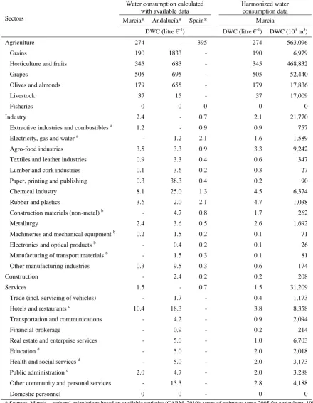
(Consejería de Medio Ambiente, 1996) and Spain (INE, 2010) to calculate Direct Water 350
Consumption (DWC) and to harmonise sectoral water consumption (Table 1). 351
352
j j x
w
DWC
(13) 353
354
Where wj is the quantity of water directly used in sector j and xj the total output of sector j.
355 356
Agricultural water productivity in Murcia is high in comparison with Andalucía and Spain. In 357
the case of Murcia, grains and olives and almonds are hardly irrigated. The bulk of water is 358
used in producing high value fruit and vegetable crops. The high DWC in Andalucía may 359
stem from significant water use in low value crops (grains) and relatively wasteful irrigation 360
techniques: 45% of irrigation is by gravity (Dietzenbacher and Velázquez, 2007). In contrast, 361
in Murcia 85% of water is supplied to crops by drip irrigation (CREM, 2011). The exception 362
to relative water use efficiency is the livestock sector which is intensive in Murcia and 363
presumably less so in Andalucía (also note that the latter figures are considerably older). 364
365
Data for industrial sectors for 1999 was updated by estimation of the 2005 level output using 366
the input-output model. Total sectoral water use was subsequently updated where sector 367
growth (positive or negative) had been such that DWC calculated with the 1999 water use 368
9
the agro-food and chemical industries, although DWC is equally high in rubber and plastics 370
and metallurgy. At the national level, DWC’s for industrial sectors are generally lower, 371
although electricity, gas and water stands out as a relatively heavy water user. The very high 372
DWC’s of the paper (including publishing and printing), chemical, and other manufacturing 373
industries reported for Andalucía were not found in Murcia. 374
375
Water use of the service sectors was redistributed according to the relative importance of 376
water consumption of these sectors in Andalucía, while respecting the total service sector 377
consumption for Murcia. Like with industrial sectors, the DWC’s thus obtained are lower 378
than those in Andalucía. Water consumption is largest in the hotel and restaurants and real 379
estate sectors, with the former having the largest DWC amongst the service sectors. 380
381
A matrix Q is defined with water inter-industry input coefficients qijcalculated as:
382 383
ij j j
i i
ij a
x w
x w
q
(if wj > 0) (14)
384
385
In analogy to Equation (1), the column totals of the inverse matrix (I-Q)-1 give the backward 386
linkages water multipliers. Forward linking water distribution coefficients lij are calculated
387
as: 388
389
ij i i
j j
ij b
x w
x w
l
(if wi > 0) (15)
390
391
The elements lij constitute matrix L; the row sums of the inverse matrix (I-L)-1 give the
392
forward linkages water multipliers. Backward linkages water multipliers represent how much 393
water is used indirectly in a given sector by considering the water consumption for its 394
intermediate consumption in relation to direct water use. Forward linkages water multipliers 395
represent the ratio of additional water use in purchasing sectors relative to the direct water 396
consumption ‘embedded’ in output from the supplying sector considered. 397
398
<<Table 1 about here>> 399
400
2.8. Water scarcity scenarios and farmers’ land use responses in Torrealvilla catchment
401
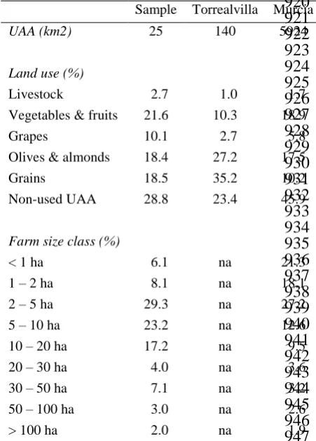
Interviews were administered with farmers within the Torrealvilla catchment (266 km2) of the 402
Guadalentin Basin in Murcia. In total 110 interviews were carried out but in the end 11 403
responses were discarded as they were incomplete. Sampling was done using the snowball 404
method, making sure all land uses were covered and an endeavour was made to represent the 405
heterogeneity of farmers in the area (Table 2). In terms of land use, in the sample livestock, 406
vegetables and fruits, and grapes are overrepresented relative to Torrealvilla and the Murcia 407
region as a whole. Small farms (< 2 ha) are heavily underrepresented, and medium farms (5-408
20ha) and fairly large farms (30-50 ha) overrepresented. Any bias in the sample is thus 409
towards viable farms which could serve the purpose of this research well given that the 410
10
final number of respondents was 7 for grains, 24 for almonds and olives, 32 for grapes, 24 for 412
horticulture and fruits and 12 for livestock. If we take agricultural census data of the Murcia 413
region as a basis for estimation, the total number of farmers in the Torrealvilla catchment 414
(which is unknown) could be 810. As extensive land uses are over- and intensive land uses 415
underrepresented in the catchment relative to the region the average farm size is likely larger 416
and the number of farmers smaller. The average farm size of our sample is 25 ha, against 17 417
ha across the Murcia region. Using this figure, the total number of farms in Torrealvilla 418
would be lower, around 560. Our sample of 99 farmers interviewed thus represents at least 419
12% and perhaps 18% of the total population. 420
421
In part, the interviews were intended to capture farmers’ responses to hypothetical scenarios 422
that reflect future uncertainty of water availability. The scenarios were developed based on 423
insights gained through discussions with farmers in the area during preliminary site visits. On 424
the one hand, concern over groundwater depletion overshadows the future of the irrigated 425
farming community. On the other hand, there have been a lot of discussions about farmers in 426
the region desperate for more water to be transferred from the North. As such, different 427
scenarios were presented to farmers who currently have access to water and those who do 428
not. The former group of farmers was asked how the following will affect the future of their 429
current principal land use: 430
Scenario A – No access to water for agricultural use (total water depletion – this could 431
occur as a physical lack of water locally, or as water quality deteriorates beyond 432
maximum tolerable salinity levels); 433
Scenario B – Government imposes tax on groundwater abstraction resulting in a water 434
price higher than maximum willingness to pay for water (WTP – lowest €0.20 m-3; 435
highest €0.60 m-3; average €0.31 m-3; standard deviation €0.08 m-3
) by individual 436
farmers; and 437
Scenario C – Government imposes tax on groundwater abstraction resulting in a water 438
price of up to the individual farmer’s maximum WTP. 439
The tax on water in scenarios B and C was presented as implying a higher price of water, a 440
situation that could also be brought about without government intervention as farmers may 441
need to pay more to obtain water in sufficient quantity and of sufficient quality. In the context 442
of this paper the maximum WTP refers to a threshold beyond which the maintenance of 443
present farming activity is perceived by individual farmers as no longer viable, making 444
drastic change such as agricultural abandonment is highly likely. Individual WTP was used as 445
cut-off point to avoid presenting multiple (fixed) price scenarios to each farmer and is 446
justified by the fact that our purpose was not to elicit farmer WTP, but to explore potential 447
land use change along a gradient of physical water scarcity (Scenario A), economic water 448
scarcity (Scenario B) and economic water insecurity (Scenario C). Farmers’ responses were: 449
1) no change; 2) conversion to other agricultural land uses; and 3) stop farming/abandonment. 450
At this point it is important to note that respondents have an incentive to understate their 451
WTP for water and/or to overstate land use changes (Carson and Groves, 2007; Schläpfer, 452
2008). As stated above, eliciting the WTP itself is not an objective of this paper, and is not 453
critical in the analysis. The fact that we ask farmers to state their hypothetical land use 454
change decisions relative to self-declared WTP minimizes the risk of exaggeration 455
(Schläpfer, 2008). Although the incentive to exaggerate may be more pronounced for water 456
price than for land use change effects of scenarios, we cannot rule out that (some) responses 457
are exaggerated; therefore the results presented should be regarded as potentially extreme 458
land use change effects. 459
460
11
agricultural land use may alter if water became available, e.g. through IBWT. This led to a 462
fourth scenario (D): 463
Scenario D1 – Water becomes available to previously non-irrigable areas. 464
At this stage, we found that grain farmers demonstrated little dynamism as compared to olive 465
and almond farmers. This is counter-intuitive, as conversion costs are considerably lower for 466
the former group. As grain farmers may have been underrepresented in the sample, we 467
therefore also defined an adjusted hypothetical scenario: 468
Scenario D2 – as Scenario D1, but for the grain farmers we adopted weights of 469
conversion to irrigated farming as elicited from olive and almond farmers (resulting in 470
increasing propensity of grain farmers to change). 471
The responses registered in Scenarios D1 and D2 were: 1) no change; 2) increase production 472
(expansion); and 3) conversion to irrigated agriculture. Note that for the purposes of 473
expansion we assumed scrubland and fallow to be available, but not forest and other land 474
uses. The effective area within the Torrealvilla catchment is thus reduced to the 140 km2 of 475
UAA. Further details about the study area and the interviews can be found in Nainggolan et 476
al. (in this issue). 477
478
<<<Table 2 about here>>> 479
480 481
2.9. Upscaling local scenario responses to the Murcia region
482
As all interviews were conducted within the Torrealvilla catchment area, we must take into 483
account the relative shares of each land use when upscaling to the Region of Murcia. We 484
thereby assume that there are no differences in the agricultural production structure of 485
subsectors between the local and regional area. 486
487
A matrix of land use changes from land use i to land use j, is constructed with elements Sji
488
defined as: 489
490
INIT i ji
ji P S
S
(16) 491
492
Where Pji is the expected probability of a change of current land use i to future land use j and 493
INIT i
S is the initial area under that land use. 494
495
The new area under land use j is subsequently obtained by summing over columns: 496
497
j ji NEW
j S
S
(17) 498
499
A vector of agricultural subsector output change as a consequence of stated land use change 500
can then be obtained by multiplying the difference in area with the output per area unit xi*:
501 502
*i INIT i NEW i
i S S x
x
(18) 503
504
Regional effects of the DCI-elicited responses to water uncertainty scenarios can now be 505
assessed with the I/O tables. We use equations (1) and (2) with vector X given by elements 506
Δxi . Total regional effects are defined as the sum of direct effects (i.e. X) and the combined
507
12 509
(f – X) + (di – X) (19)
510 511
An analogous procedure (Equations 18-19) is followed to assess the direct and indirect 512
effects of the changed total sector water demands Δwi .
513 514
2.10. Effect of increased water cost on sector unitary output prices
515
With the preceding steps, we can now simulate the impact of increased water costs on sector 516
unitary output prices. We will assume that increased costs for water only apply to agricultural 517
water use, assuming that other sectors already pay more for water (e.g. twice as much in 518
neighbouring Almería province – Downward and Taylor, 2008). 519
520
VWM’ = DWCp’ (I-A)-1 (20)
521 522
Where the vector VWM is the Virtual Water Multiplier (the accent (’) indicates transposition) 523
found by multiplying the vector DWCp – consisting of DWC for sectors where the water 524
price will be raised (i.e. agricultural subsectors) and 0 for other sectors – with the Leontief 525
inverse matrix. The VWM can subsequently be used to calculate a price increase by simple 526
multiplication (the VWM can directly be interpreted as representing a price increase of €1). 527
We will present the effects of a price increase of €0.10 m-3 – equal to the average incremental 528
WTP (€0.04 m-3) plus one standard deviation (€0.06 m-3
) to account for possible 529
understatement (the range of incremental WTP was €0.00–0.25 m-3). The cumulative effects 530
of the water price increase, through water input-output relations, on product prices can help to 531
understand farmer responses to the discrete choice scenarios. 532
533 534
3. Results
535 536
3.1. Regional I/O Table for Murcia
537
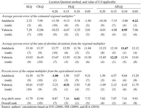
The regional I/O table constructed for Murcia was evaluated by applying the same method to 538
neighbouring autonomous regions for which survey-based I/O tables were available: 539
Andalucía and Valencia. Table 3 shows the results of different methods. The average regional 540
multiplier is overstated by the SLQ and CILQ methods (in line with findings by others – 541
Boomsma and Oosterhaven, 1992; Flegg and Tohmo, in press), but more so for Valencia than 542
for Andalucía. In contrast, FLQ and AFLQ methods lead to a general understatement except 543
at low values of δ. The absolute average deviations from the regional multiplier show an error 544
of 13.2-16.5% for SLQ and CILQ. FLQ and AFLQ methods with appropriate scaling factor δ 545
can moderately reduce this error to about 12%. Contrary to findings by Flegg and Tohmo (in 546
press), the AFLQ outperforms the FLQ in these two cases, although overall error reductions 547
are not as large as these authors suggest. When zooming in on the accuracy of predicting the 548
regional output multiplier for the agricultural sector, the overstatement errors of the 549
conventional SLQ and CILQ approaches are larger than for the total regional economy. Both 550
the FLQ and AFLQ can greatly reduce errors in estimating the agricultural output multiplier, 551
to about 1%. Higher values of the scaling factor δ attain largest error reductions, whereby 552
AFLQ is more prone to exaggerating the multiplier than FLQ. Taking into account: a) the 553
need to have a low average absolute deviation of the average regional multiplier; b) a 554
preference for a slight underestimation of the average regional multiplier; c) the trend 555
observed in literature that smaller regions (such as Murcia) have a higher propensity to have a 556
lower optimal value for δ; and d) that such a trend would place an optimal δ for Murcia’s 557
13
percent error for the six data rows in Table 3 is lowest for FLQ with δ = 0.10 (see overall 559
rank), we applied FLQ with δ = 0.10 to develop a non-survey based regional input-output 560
table for Murcia. 561
562
<<<Table 3 about here>>> 563
564
3.2 The regional I/O Table with disaggregated agricultural sector
565
Table 4 shows details about the disaggregation of agriculture in five subsectors at the regional 566
scale. All subsectors except livestock occupy sizeable shares of the region’s agricultural area 567
(11-36%). However, in terms of output value, grains (2%), grapes (5%) and olives and 568
almonds (5%) contribute only modestly compared with livestock (22%) and especially 569
vegetables and fruits (66%). As a result, productivity per area unit ranges widely. Production 570
structures of the subsectors are therefore also expected to vary considerably. The backward 571
output multipliers of individual subsectors of the disaggregated I/O table varied between 1.22 572
for vegetables and fruits and 1.86 for livestock (Table 5). The first reflects that relatively little 573
economic activity is generated by producing an Euro worth of horticultural produce, whereas 574
the opposite holds for livestock. The disaggregated I/O table was also tested for its similarity 575
with the aggregated version: when scaling the five subsectors, its combined agricultural 576
sector backward output multiplier is in both cases 1.38. Similarly, the forward output 577
multiplier of the current (2005) sector configuration is 1.60. Individual agricultural sectors 578
have forward multipliers of 2.11-2.28, which demonstrates that much of their produce is sold 579
to upstream industries. The vegetables and fruits subsector (1.31) is an exception, as produce 580
is not processed in agro-industries but marketed to consumers and – importantly – exported. 581
For all agricultural subsectors, forward linkages are higher than backward linkages. Agro-582
food industries and construction are sectors with high backward linkages, whereas 583
construction materials and lumber industries have high forward linkages. 584
585
<<<Table 4 about here>>> 586
<<<Table 5 about here>>> 587
588
3.3. Regional I/O Table of water use
589
Agriculture consumes about 80% of total (‘blue’) water use in Murcia: households consume 590
about 15%; and other economic sectors together account for only 5%. Not surprisingly, 591
technical coefficients of water use are a fraction of the technical coefficients based on the 592
monetary value of intermediate consumption (cf. Equation 14). The water multipliers (both 593
backward and forward) of the agricultural subsectors are thus low in comparison to output 594
multipliers (Table 5). Livestock is the subsector with the highest backward water multiplier 595
(1.65): its intermediate consumption relies on water-intensive inputs. Grains have the highest 596
forward multiplier (1.28): the sectors grains are supplied to use a considerable amount of 597
water, whereas water needs for grains are relatively low. Similarly, vegetables and fruits have 598
the lowest non-zero forward water multiplier (1.03). Very little additional water is used to 599
produce output in processing sectors (which moreover absorb only a limited part of total 600
vegetables and fruits output). 601
602
The modest water multipliers for agricultural subsectors contrast with some of the water 603
multipliers in industries and services. Backward multipliers are very high for lumber and cork 604
industries (33.71), agro-food industries (13.60), and paper, printing and publishing (10.74). 605
These sectors thus require water-intensive inputs totalling several times their direct water 606
demand. Machineries and mechanical equipment (23.06) and financial brokerage (18.46) 607
14
amounts of water, but the output of purchasing sectors requires a multiple factor total water 609
input. 610
611
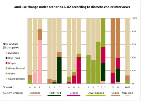
3.4. Discrete choices and land use change scenarios in Torrealvilla
612
When farmers with current access to water were asked what their strategy would be if water 613
resources would be completely depleted, the vast majority would give up farming (Figure 2, 614
Scenario A). A sizeable minority (43%) of olive and almond farmers would not change land 615
use, a strategy also followed by 3% of vineyard managers (these crops can be grown without 616
irrigation, obviously with reduced productivity; for vineyards a change from table to wine 617
grapes may be involved, as well as introduction of supplementary drip irrigation). Remaining 618
farmers would resort to rainfed cropping. A similar pattern emerged when the same group of 619
farmers was confronted with high (perceived) water taxation (Scenario B); again the most 620
common response was abandonment. Continuation of the current land use was the preferred 621
strategy of 36% of olive and almond farmers, 17% of livestock farmers, 12% of vineyard 622
managers and only 2% of horticulturalists and fruit growers. Some vineyards and fruit 623
orchards would convert to olive and almond groves and grains, respectively. Under low 624
(perceived) water taxation (Scenario C) the majority (67% and 64%) of livestock and olive 625
and almond farmers would continue current land use. However, 54% of vineyard managers 626
and 52% of horticulturalists and fruit growers stated that they would abandon their 627
enterprises. In both cases, 40% would continue. Some 17% of livestock farmers and 8% of 628
horticulturalists and fruit growers would opt for a change to grains, and 5% of vineyard 629
managers would switch to olives and almonds. These three discrete choice scenarios show 630
that water availability and affordability is a crucial factor for all with current access to water. 631
Horticulture and fruit growing, vineyards and livestock farming are the least likely to flourish 632
under physical or economic water scarcity. 633
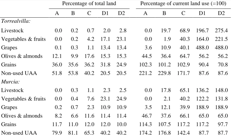
Figure 2 also shows scenarios presented to farmers who currently do not have access to 634
water. If a new IBWT project would be realized, some unused land would start to be 635
cultivated to grains (8%) and olives and almonds (5%). Olive and almond groves would see 636
considerable conversion to horticulture and fruit growing (24%) and vineyards (21%). 637
Moreover, 14% of grain fields would be developed to vineyards. Overall, olive and almond 638
farmers demonstrated the most dynamic choices. If the changes expressed above were to 639
occur, land use in the Torrealvilla catchment would change as shown in Table 6. 640
641
<<<Figure 2 about here>>> 642
<<<Table 6 about here>>> 643
644
3.5. Regional effects of land use change scenarios
645
When we simulate the effects of the discrete choice scenarios in the input-output model, the 646
land use change scenarios driven by uncertainty in water supply result in diverging effects on 647
regional economy and water demand (Figure 3). The total water depletion scenario almost 648
eradicates the agricultural sector, and when taking into account forward and backward 649
linkages leads to a shrinking of the regional economy of 14%. As all irrigated agriculture 650
disappears in this scenario, this scenario reduces the demand for water to about 18% of the 651
current level. A high water tax has just slightly lower impact. A low water tax impacts the 652
regional economic output by 7% while reducing water demand to almost half the current 653
level. A new water transfer may lead to 4-5% economic growth while requiring 23-30% more 654
water compared to current regional demand. The ratio of economic impact to water demand 655
reveals interesting results. When left to abandonment because of a total depletion of water, 656
15 high water tax this ratio is reduced to €5.36 per m3
, whereas a low water tax results in a loss 658
of €4.85 per m3
. Increased water availability similarly augments regional economic output by 659
€5.63-5.86 per m3 . 660
661
<<<Figure 3 about here>>> 662
663
3.6 Water price effects
664
Table 7 shows the effects of ‘acceptable’ agricultural water price increase on the product 665
price of each sector. Although the horticulture and fruits subsector uses more water, it 666
produces more output per unit of water and hence the effects of water price increases are not 667
as pronounced as for grapes and olives and almonds. The ‘acceptable’ water price increase 668
represents almost 50% of the currently paid average price and leads to agricultural product 669
price increases between 0.6 and 5.6%, with three out of five subsectors being affected by over 670
3%. Agro-food (0.4%) and lumber and cork (0.1%) industries are the two non-agriculture 671
sectors where a price effect is notable. 672
673
<<<Table 7 about here>>> 674
675 676
4. Discussion
677 678
The I/O table for Murcia needed to be constructed first in order to enable subsequent scenario 679
analyses. We evaluated several location quotient methods: SLQ, CILQ, FLQ and AFLQ. Our 680
results concur with other studies that find conventional SLQ and CILQ methods to 681
overestimate multipliers. Because the agricultural sector in Murcia and – to lesser extent – 682
neighbouring regions is so dependent on exports, extra prudence proved to be required, and 683
the appropriate scaling method (value of parameter δ = 0.10) for FLQ was well below the 684
usual range (0.25 ± 0.05) reported by Flegg and Tohmo (in press), supporting their remark 685
that individual cases need special scrutiny. Without availability of survey-based I/O tables for 686
neighbouring regions, we would probably have run a high risk of substantially overstating 687
impacts of scenarios. The methods described for disaggregating the agricultural sector and 688
constructing the water I/O table can, given similar data availability, more confidently be 689
applied in other contexts. 690
691
The ratio of economic impact to water demand (Figure 3) can be interpreted as follows: when 692
confronted with high barriers to water use (total depletion, high water tax), farmers tend to 693
give up farming. In these cases the economic consequences are high in relation to changes in 694
regional water demand. However, the introduction of a low water tax prompts a significant 695
number of farmers to change land use instead of abandonment. As a consequence, reductions 696
in water use are obtained, resulting in about 10% lower impact on the regional economy per 697
unit of water saved than under a higher water tax scenario. Potential water savings are 698
impressive: a low water tax can reduce total water demand by almost 50% (note this is only 699
considering responses by agricultural agents) at a 7% cost to the regional economy. Tax 700
revenues could be used to stimulate further water savings, or to develop economic activities 701
with a low water use. Important gains can be achieved in setting the water tax level right: our 702
study suggests that significant water savings can be achieved at relatively low expense to the 703
regional economy by incentivising self-organizing capacity of the agricultural sector – i.e. 704
through land use changes as described above. Stronger intervention (through higher taxation) 705
fails to take advantage of this self-organizing capacity and although it may generate higher 706
16 first place.
708 709
There may however be limits to the capacity of the system to self-organize and adapt to 710
groundwater scarcity if this scenario is combined with future climate change. Increased 711
temperatures would increase evaporation and evapotranspiration rates and hence further 712
increase water demand. If climate change leads to reduced rainfall inputs, this would not only 713
reduce groundwater recharge rates, perhaps hastening groundwater scarcity, but also limit the 714
viability of switching from irrigated to rainfed agriculture. 715
716
Given the questionable sustainability of groundwater extraction rates, it is of particular 717
concern that agriculture in Murcia has become so heavily dependent on this finite and 718
dwindling resource. Our results show that without groundwater and IBWT, about two-thirds 719
of the region’s agricultural area would be abandoned. Agricultural output would be 720
decimated to less than 5% of its current value. Even the introduction of a low water tax would 721
still lead to about 35% of the agricultural area being abandoned, with an associated loss of 722
more than half of the current output. Whereas our farmer survey using discrete choice 723
scenarios may have led to exaggerated responses, this clearly illustrates how vulnerable 724
respondents feel to uncertainty in water supply. Our data do not show margins on crops 725
grown, but the intermediate consumption of the five subsectors we distinguished varied 726
between 16% (horticulture and fruits) and 50% (livestock) of output value. When adding 727
labour costs and imports, margins may be narrow. Any water taxation (or scarcity, for that 728
sake) can under these circumstances lead to heated debate. Surprisingly, results of increased 729
water prices (Table 7) have the highest impact on grapes and almonds and olives. This 730
contrasts with the land use decisions elicited from DCI interviews, where horticulture and 731
fruits are the first to be abandoned or switched. Although our results are not conclusive, this 732
could indicate that the latter crops are perceived by farmers as more sensitive to water 733
shortages. 734
735
Additional water supply through IBWT may lead to a 10% expansion of the agricultural area, 736
with an associated increase in agricultural output of 26-35%. Given the high export 737
orientation and strong regional agro-food industry it is not unreasonable to assume this 738
additional produce could be effectively handled (cf. Sánchez-Chóliz and Duarte, 2000). The 739
ratio of economic impact to increased water demand of such an expansion is high (€5.63-5.86 740
per m3), suggesting that additional water will be used efficiently and an accelerated growth 741
may result. The economic multiplier is, at 1.75, higher than currently obtained, reflecting the 742
combined effect of water and extra land as production factors. Although this sounds 743
promising, it further increases water-dependency of the regional economy. It should be noted 744
though that the assumption of stable technical coefficients inherent to input-output models 745
might be too optimistic here as the best land is probably already irrigated and land onto which 746
irrigation can be expanded may not be as productive as the currently irrigable area. 747
Strikingly, the farmers’ discrete choices may reflect this fact, with only a minority of grain 748
farmers and slightly over half of olive and almond farmers envisioning land use changes to 749
horticulture and fruits or vineyards. 750
751
We can also take a closer look at the currently operational Tagus–Segura IBWT scheme 752
(Figure 4). In 1994/5 and 2005-7, the amount of water transferred was greatly reduced as a 753
consequence of the distribution rules in place to cap transfer if the conceding basin 754
experiences water shortage. In the latter period, the contribution of the IBWT to total 755
irrigation dropped to 8% from 54% in 2002/3. This massive reduction is partly compensated 756
17
exploited. The drop in total irrigation may point at a number of potential issues: a) pumping 758
capacity installed is too low to fully compensate for significant reductions in IBWT water; b) 759
not all areas benefiting from the IBWT can switch to groundwater resources if required; or c) 760
the economic cost of pumping exceeds (€0.12 – €0.54 m-3) by far the price (€0.09 m-3 ) paid 761
for IBWT water (Tobarra González, 2002). Although a mix of these issues may have 762
occurred, and farmers may also have adapted in anticipation of lower water availability, the 763
clear peak of local irrigation (levelling off since 2008) clearly suggests that a sizable number 764
of farmers have been willing to pay an additional €0.03 to €0.36 per m3
water. This is in good 765
agreement with our field data. Alternative mobilisation of additional water resources is more 766
expensive: the most cost-effective desalinisation plants may produce water at a cost of €0.45 767
m-3, and the Ebro–Segura IBWT would charge an average of €0.31 m-3 along the pipeline, 768
rising to an expected €0.75 m-3 in Almeria (Downward and Taylor, 2008). Desalinisation 769
could be partly subsidised by the government as it can relieve social and environmental 770
problems associated with the current IBWT and groundwater overexploitation. However, 771
average energy demands of desalinisation are more than a factor of 3 higher than for the 772
Tagus-Segura IBWT and lead to an increased environmental cost of CO2 emissions of €0.07 773
per m3 of desalted water (Melgarejo and Montano, 2011), as well as increased coupling of 774
water to volatile energy prices. 775
776
<<<Figure 4 about here>>> 777
778
As most of the additional output resulting from IBWT will leave the region with exports as 779
virtual water, it is from an environmental perspective a questionable development pathway. 780
Currently, the economy of Murcia produces €39.26 per m3 of water used – over 8 times as 781
efficient as would be achieved with new IBWT development. As a consequence, the regional 782
economic output per cubic metre of water would drop below €30. Compare that with the over 783
€90 per m3
that results from the low water tax and it is clear that better alternatives are 784
available. Admittedly, the first option leads to regional economic growth of 4.4% while the 785
latter to a contraction of 6%, but intermediate solutions should be available that warrant 786
growth while improving water use efficiency. 787
788 789
5. Conclusion
790 791
Agriculture in the Region of Murcia has increasingly become dependent on blue water 792
resources. Current water availability for irrigation is threatened by continuous 793
overexploitation of groundwater resources, increased competition from non-agricultural (and 794
in some cases illegal) uses, and conflicts over inter-basin water transfer – all in the context of 795
global environmental change. The regional government has a tremendous challenge to reduce 796
overexploitation of water resources and reduce vulnerability of the regional economy to water 797
scarcity. At the same time, the region’s farmers feel trapped in water-dependent productivity 798
and fear any reform that negatively affects their resource base. We evaluated the effects of 799
farmers’ responses to discrete choice scenarios on the regional economy and water demand 800
by means of input-output modelling. Our results confirm that agriculture is heavily dependent 801
on blue water resources, and farmers see no option to continue farming if confronted with 802
complete water depletion (physical water scarcity) or high levels of water taxation (economic 803
water scarcity). These scenarios would lead to very large reductions in water use by 804
agriculture, but also result in a contraction of the regional economy by more than 13%. A low 805
water tax scenario indicated that some farmers may change land use as a result. Although still 806