Comparison and development of machine learning tools in the prediction of chronic kidney disease progression

RESEARCH

Comparison and development of machine

learning tools in the prediction of chronic

kidney disease progression

Jing Xiao

_{, Ruifeng Ding}

_{, Xiulin Xu}

_{, Haochen Guan}

_{, Xinhui Feng}

_{, Tao Sun}

_{, Sibo Zhu}

and Zhibin Ye

Abstract

Background: Urinary protein quantification is critical for assessing the severity of chronic kidney disease (CKD). How-ever, the current procedure for determining the severity of CKD is completed through evaluating 24-h urinary protein, which is inconvenient during follow-up.

Objective: To quickly predict the severity of CKD using more easily available demographic and blood biochemical features during follow-up, we developed and compared several predictive models using statistical, machine learning and neural network approaches.

Methods: The clinical and blood biochemical results from 551 patients with proteinuria were collected. Thirteen blood-derived tests and 5 demographic features were used as non-urinary clinical variables to predict the 24-h urinary protein outcome response. Nine predictive models were established and compared, including logistic regression, Elastic Net, lasso regression, ridge regression, support vector machine, random forest, XGBoost, neural network and k-nearest neighbor. The AU-ROC, sensitivity (recall), specificity, accuracy, log-loss and precision of each of the models were evaluated. The effect sizes of each variable were analysed and ranked.

Results: The linear models including Elastic Net, lasso regression, ridge regression and logistic regression showed the highest overall predictive power, with an average AUC and a precision above 0.87 and 0.8, respectively. Logistic regression ranked first, reaching an AUC of 0.873, with a sensitivity and specificity of 0.83 and 0.82, respectively. The model with the highest sensitivity was Elastic Net (0.85), while XGBoost showed the highest specificity (0.83). In the effect size analyses, we identified that ALB, Scr, TG, LDL and EGFR had important impacts on the predictability of the models, while other predictors such as CRP, HDL and SNA were less important.

Conclusions: Blood-derived tests could be applied as non-urinary predictors during outpatient follow-up. Features in routine blood tests, including ALB, Scr, TG, LDL and EGFR levels, showed predictive ability for CKD severity. The developed online tool can facilitate the prediction of proteinuria progress during follow-up in clinical practice.

© The Author(s) 2019. This article is distributed under the terms of the Creative Commons Attribution 4.0 International License (http://creat iveco mmons .org/licen ses/by/4.0/), which permits unrestricted use, distribution, and reproduction in any medium, provided you give appropriate credit to the original author(s) and the source, provide a link to the Creative Commons license, and indicate if changes were made. The Creative Commons Public Domain Dedication waiver (http://creat iveco mmons .org/ publi cdoma in/zero/1.0/) applies to the data made available in this article, unless otherwise stated.

Background

Chronic kidney disease (CKD) is associated with an increased risk for adverse clinical events, which makes it

a major public health problem worldwide [1]. Although it is well recognized that CKD is independently associated with increased risks for end stage renal disease, cardio-vascular events, and all-cause mortality, the prognosis for individual patients still lacks sufficient information [2]. Clinically usable strategies for the risk stratification of each outcome are important for making treatment deci-sions [3, 4].

Renal prognosis predictive models in CKD patients may be helpful in identifying those at high risk who may

Open Access

*Correspondence: [email protected]; [email protected] †_{Jing Xiao and Ruifeng Ding contributed equally to this study} 1 _{Department of Nephrology, Huadong Hospital Affiliated To Fudan} University, Shanghai 200040, China

4 _{MOE Key Laboratory of Contemporary Anthropology, School of Life} Sciences, Fudan University, Shanghai 200438, China

benefit from more intensive management, such as higher doses of RAAS (renin–angiotensin–aldosterone system) inhibitors, anticoagulation therapy, and intensive blood glucose, blood pressure, urate and lipid-lowering medi-cations [5]. In addition, how to screen outpatient CKD patients who should have intensive and quick examina-tions is of great clinical and economical significance. With the use of such models, most patients with risks of having proteinuria less than 1  g/24  h can be strati-fied as low risk and can potentially be treated solely by their primary outpatient follow-up, whereas those at high risk (proteinuria more than 1  g/24  h) can be referred to urgent care by an inpatient management registra-tion. Similarly, models predicting renal progression may identify patients at low risk for renal failure in the next 5 years, for whom advanced treatment may be inappro-priate [6]. Proteinuria has always been recognized as the most important risk factor [7]. A recent study improved the prediction efficacy by using proteinuria to estimate the glomerular filtration rate [8]. However, models using proteinuria need to collect the 24-h urine, which is inconvenient, especially in outpatient clinics.

Studies have been conducted to try to use routinely obtained laboratory tests without proteinuria to predict renal progression. Models including age, sex, estimated GFR, albuminuria, serum calcium, serum phosphate, serum bicarbonate, and serum albumin can accurately predict the progression to kidney failure in patients with CKD stages 3–5 [4]. More recently, artificial intelligence approaches have been proven to solve real problems, including rule-based and gold standard oriented diag-noses or progdiag-noses. To help clinicians select prediction tools for predicting the severity of CKD, we established and compared nine prediction models using statistical, machine learning and neural network approaches with blood-derived outpatient clinical features and demo-graphic features. Based on the results, we further estab-lished an online tool for patient follow-up urinary protein severity prediction.

Methods and materials Patients and data pre‑processing

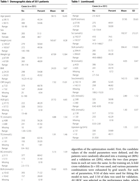
A total of 551 pathologically confirmed CKD patients with 24-h urinary protein were recruited from August 2015 to September 2018 at the Department of Nephrology in the Shanghai Huadong Hospital Affiliated to Fudan Univer-sity. None of the patients were diagnosed with METS, can-cers or cardio- and cerebrovascular diseases. The detailed demographic characteristics of the cohort are listed in Table 1. In this study, urine protein > 1 g/24 h was used as the outcome variable to classify the progress and severity of proteinuria in patients with kidney disease. Our study was approved by the Clinical Ethics Review Committee of the

Shanghai Huadong Hospital Affiliated to Fudan University, and clinical consent was obtained from all patients. We first cleaned and formatted the data before model fitting. Then, in the pre-processing stage, we transformed categorical variables into binary dummy variables. Finally, we scaled the data as most models are affected by the difference in the scale of the variables. We performed power analysis over urinary protein values to determine if the sample size was suitable for further statistical process (alpha = 0.05). All val-ues were normalized to reduce the dimension-introduced bias using Z-score standardization as previously described [9–13]: (Eq. 1).

where μ is the average of the features across all samples, and α is the standard deviation.

Establishment of a predictive model

In this study, nine predictive models were established to predict the progression of urinary protein in patients with chronic kidney disease, and model selection was based on several currently and frequently adopted predictive model types. For the linear model, the logistic regression model (LR) [14, 15], the elastic network model (Elastic Net) [16–

18], the lasso regression model (Lasso) [19], and the ridge regression model (Ridge) were selected [20–22]. The neu-ral network model (NN) [23] was chosen because it is an important class of nonlinear prediction models [24] and has been reported to predict CKD. For the kernel-based model, a support vector machine (SVM) with a Gauss-ian kernel (RBF) has been widely adopted in many clini-cal applications, such as coronary artery disease prediction [25, 26]. For the decision tree approach, the random forest (RF) model [27–29] and the XGBoost model [30–32] have also been used in clinical research. Finally, a basic predic-tion technique [33], k-nearest neighbor algorithm (k-NN) was built [34]. The model was fitted using the method described above for each set of parameters, which were adjusted to obtain the average performance index. The log-loss was calculated to indicate the confidence of the model. The lower the log-loss value is, the more confident the model is for its classification results [35, 36]. The technical parameters of the selected prediction models are listed for the optimization of the equations (Table 2). Model estab-lishment and brief illustrations are described in Additional file 1.

Assessment of models in CKD severity prediction

In this study, we have improved the method of the data resampling technique [37] considering the overfit-ting problem caused by the empirical risk minimization

(1)

z₌ x−µ

algorithm of the optimization model. First, the candidate values of the model parameters were defined, and the patients were randomly allocated into a training set (80%) and a validation set (20%), where the two class propor-tions in each set were the same. In the training set, k-fold cross-validation (k = 10) was used, and various parameter

combinations were exhausted by grid search. For each set of parameters, 9/10 of data were used for fitting the model in turn, and 1/10 of data was used for validation. AU-ROC was selected as the performance index, which Table 1 Demographic data of 551 patients

Cases (n = 551)

No Percent Mean SD

Age (years) 58.15 16.45

≤ 58.15 251 45.54

> 58.15 300 54.46

Range 18–90

Sex

Male 283 51.3

Female 268 48.7

Height (cm) 165.67 8.28

≤ 165.67 279 50.64

> 165.67 272 49.36

Range 145–190

Weight (g) 67.09 12.84

≤ 67.09 286 51.91

> 67.09 265 48.09

Range 39–118

BMI 24.33 3.67

≤ 24.33 298 54.08

> 24.33 253 45.92

Range 16.23–41.32

CRP (mg/L) 7.32 15.01

≤ 7.32 379 68.78

> 7.32 147 26.68

Missing 25 4.54

Range 0–190

ALB (g/L) 37.72 6.65

≤ 37.72 222 40.29

> 37.72 328 59.53

Missing 1 0.18

Range 13–66

TC (mmol/L) 4.88 1.54

≤ 4.88 310 56.26

> 4.88 231 41.92

Missing 10 1.81

Range 1.30–12.93

TG (mmol/L) 1.91 1.46

≤ 1.91 348 63.16

> 1.91 193 35.03

Missing 10 1.81

Range 0.4–18.2

BG (mmol/L) 5.13 1.59

≤ 5.13 377 68.42

> 5.13 173 31.40

Missing 1 0.18

Range 2.3–17.5

BUN (mmol/L) 10.42 8.35

≤ 10.42 393 71.32

> 10.42 157 28.49

Missing 1 0.18

Table 1 (continued)

Cases (n = 551)

No Percent Mean SD

Range 2.5–62.0

EGFR (ml/min) 57.95 35.63

≤ 57.95 275 49.91

> 57.95 276 50.09

Range 1.0–154.4

Scr (umol/L) 192.57 212.21

≤ 192.57 410 74.5

> 192.57 141 25.5

Range 41.9–1460.7

SUA (umol/L) 394.41 110.63

≤ 394.41 285 51.72

> 394.41 266 48.28

Range 49.0–808.0

SK (mmol/L) 4.03 0.47

≤ 4.03 306 55.54

> 4.03 241 43.74

Missing 4 0.72

Range 2.7–5.6

Sna (mmol/L) 142.13 3.08

≤ 142.13 289 52.45

> 142.13 258 46.82

Missing 4 0.72

Range 108.2–152.0

LDL (mmol/L) 2.80 1.12

≤ 2.80 325 58.98

> 2.80 226 41.02

Range 0.42–8.95

HDL (mmol/L) 1.30 0.37

≤ 1.30 317 57.53

> 1.30 233 42.29

Missing 1 0.18

Range 0.53–2.81

Uprotein (g/24 h) 1.55 2.21

≤ 1.0 330 59.89

> 1.0 221 40.11

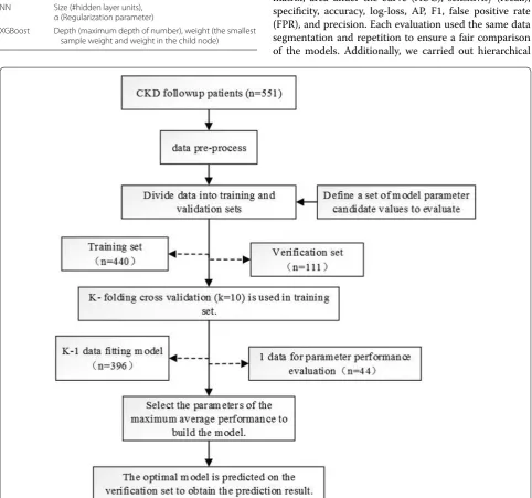
was calculated 10 times, and its average performance was calculated as the parameter score of the current param-eter combination. The average value of the paramparam-eter value grid was selected as the best performance adjust-ment parameter of the current iteration and was finally executed on the test set. A forecast flow chart is shown in Fig. 1. This step was repeated 20 times randomly, i.e., 20 resampling iterations were defined. This study used the same resampling to evaluate different models. For each model, the evaluation indicators used were the confusion matrix, area under the curve (AUC), sensitivity (recall), specificity, accuracy, log-loss, AP, F1, false positive rate (FPR), and precision. Each evaluation used the same data segmentation and repetition to ensure a fair comparison of the models. Additionally, we carried out hierarchical Table 2 Tuning parameters of the predictive models

Models Tuning

LR α (Regularization parameter) Elastic Net γ (Mixing percentage),

α (Regularization parameter) Lasso α (Regularization parameter) Ridge α (Regularization parameter) SVM γ (Gaussian kernel), C (Cost) RF n_estimators (#subtrees)

k-NN k (#Neighbors)

NN Size (#hidden layer units), α (Regularization parameter)

XGBoost Depth (maximum depth of number), weight (the smallest sample weight and weight in the child node)

clustering analysis over methods based on false positive (FP) and false negative (FN) values. In this study, Python (version 3.7.0) and R (version 3.5.1) were used to build and evaluate the models.

To better evaluate the performance of the models, we further compared the AU-ROC from each resampling calculation using a paired t test. P < 0.05 was regarded as significant. In addition to performance comparisons, this study also analysed the importance of variable fac-tors in the predictive models. For each model, the relative effect size was quantified by assigning a weight between 0 and 1 for each variable. The models XGBoost and RF allowed the importance of variables to be derived during model training; the coefficients of the Elastic Net, Lasso, and Ridge models were used as the importance factor. For models, such as kNN and SVM, wherein the impor-tance of variables was difficult or impossible to extract,

the mean decrease accuracy was obtained by directly measuring the effect of each feature on the accuracy of the model. Briefly, the model was fitted, and parameter adjustment was performed to predict the validation set to obtain the model performances. Then, the feature values were disturbed to establish a new disturbance prediction set. Obviously, for the unimportant variables, the scram-bling order has little effect on the accuracy of the model, but for the important variables, the scrambled order will reduce the accuracy of the model. Finally, the relative importance ratio of all the eigenvalues was given a weight between 0 and 1 according to the overall proportion, thereby obtaining the effect sizes.

Establishment of web tools for CKD severity prediction

the above models whose predictive precision, sensitiv-ity and specificsensitiv-ity were highest. The proteinuria predic-tor was embedded in the web tool. User data interaction and visualization of analysis results were displayed using HTML5, JavaScript, and PHP. Source codes for model establishment by Python and web tools by PHP are pro-vided in Additional file 1.

Results

Patients and variables

This study recruited 551 patients with CKD from the Department of Nephrology, Huadong Hospital, Shang-hai Fudan University Affiliated Hospital who had patho-logically confirmed 24-h urine protein. The training dataset included 330 mild CKD patients (urinary pro-tein ≤ 1 g/24 h) and 221 moderate/severe CKD patients

(urinary protein ≥ 1  g/24  h). Through statistical power

analysis of the urinary protein values, the sample size in

our study was competent for further procedures with power at 1. The following non-urine indicators of 13 outpatient blood biochemistry tests and 5 demographic features were used as predictive variables: CRP, ALB, TC, TG, BG, BUN, EGFR, Scr, SUA, SK, Sna, LDL, HDL, sex, age, height, weight, and BMI. Urine protein (g/24 h) was considered an outcome variable to judge the status of CKD patients.

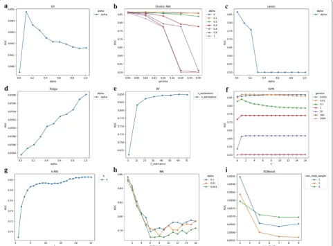
Tuning of parameters

The average AU-ROC for different models and their parameters are listed (Fig. 2). The SVM was not sensi-tive to cost choice C, and the kernel smoothing param-eter σ of 0.01 was optimal. For k-NN, a relatively large number of k = 24 was optimal; for RF, a relatively large

sample weight (min_child_weight) of 1 achieved optimal performance.

Validation of the training set

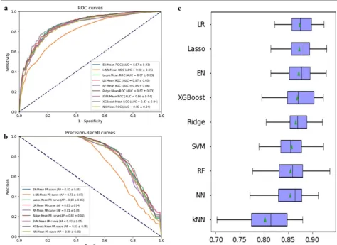
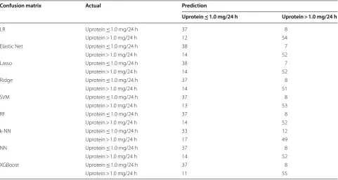
The average ROC curves and PR curves during the 20-fold data resampling process are shown in Fig. 3a, b. Most models had AUC values above 0.85, but the value of k-NN was lower (0.80). We used the AP value as the criterion for the PR curve [38]. The APs of the Elastic Net, Lasso, LR, Ridge, SVM and XGBoost models were all above 0.82. The confusion matrix (rounding) was also calculated for the nine models (Table 3). As shown in

Table 3, k-NN generated a large amount of FNs (= 12) and FPs (= 17) during the prediction process, while the other models had the same number of FNs, which could be controlled within 10, where the Lasso and Elastic Net models produced the least amount of FNs (= 7). The model XGBoost produced the minimum number of FPs (= 11).

The nine methods were clustered based on hierarchi-cal clustering analysis using the FP and FN values from one random sampling (Additional file 1: Figure S1). Simi-lar models drew simiSimi-lar results; for example, the decision tree models XGBoost and random forest were clustered Table 3 Confusion matrices of 9 models

Confusion matrix Actual Prediction

Uprotein ≤ 1.0 mg/24 h Uprotein > 1.0 mg/24 h

LR Uprotein ≤ 1.0 mg/24 h 37 8

Uprotein > 1.0 mg/24 h 12 54

Elastic Net Uprotein ≤ 1.0 mg/24 h 38 7

Uprotein > 1.0 mg/24 h 14 52

Lasso Uprotein ≤ 1.0 mg/24 h 38 7

Uprotein > 1.0 mg/24 h 14 52

Ridge Uprotein ≤ 1.0 mg/24 h 37 8

Uprotein > 1.0 mg/24 h 14 51

SVM Uprotein ≤ 1.0 mg/24 h 37 8

Uprotein > 1.0 mg/24 h 13 53

RF Uprotein ≤ 1.0 mg/24 h 37 8

Uprotein > 1.0 mg/24 h 14 52

k-NN Uprotein ≤ 1.0 mg/24 h 33 12

Uprotein > 1.0 mg/24 h 17 49

NN Uprotein ≤ 1.0 mg/24 h 37 8

Uprotein > 1.0 mg/24 h 14 52

XGBoost Uprotein ≤ 1.0 mg/24 h 37 8

Uprotein > 1.0 mg/24 h 11 55

Table 4 Performance summary in terms of AU-ROC sensitivity (recall), specificity, accuracy, log-loss, FP rate, precision

Models AUC 95%CI Sensitivity

(recall) Specificity Accuracy log‑loss FP rate Precision AP F1 Lower bound Upper bound

LR 0.873 0.808 0.939 0.83 0.82 0.82 6.16 0.18 0.76 0.83 0.79

Elastic Net 0.871 0.805 0.937 0.85 0.80 0.82 6.29 0.20 0.74 0.82 0.79

Lasso 0.872 0.807 0.938 0.84 0.79 0.81 6.41 0.21 0.74 0.82 0.79

Ridge 0.865 0.798 0.933 0.83 0.79 0.81 6.71 0.21 0.73 0.82 0.78

SVM 0.857 0.786 0.928 0.82 0.81 0.81 6.50 0.19 0.75 0.82 0.78

RF 0.854 0.782 0.926 0.83 0.79 0.80 6.77 0.21 0.73 0.81 0.77

k-NN 0.802 0.721 0.883 0.74 0.74 0.74 8.91 0.26 0.69 0.73 0.70

NN 0.854 0.783 0.925 0.83 0.78 0.80 6.91 0.22 0.73 0.80 0.77

closely. Table 4 shows the AUC, sensitivity (recall), speci-ficity, accuracy, log-loss, FP rate, precision, f1, and AP of each model evaluation result.

There were significant performance differences between the different models (Fig. 3c and Table 4). The linear models LR, Elastic Net, Lasso and Ridge had excellent performance, and the accuracy rate was up to 0.80. Among them, LR obtained the highest AUC value of 0.873, and the tree model XGBoost had an AU-ROC value of 0.868 and an accuracy rate of 0.83. K-NN obtained the lowest AUC value of 0.802. The best perfor-mance of sensitivity was the Elastic Net model, which is suitable for the early diagnosis of proteinuria progression in patients with chronic kidney disease. The best particu-larity was XGBoost and LR, which are suitable for the early stage of proteinuria in patients with chronic kidney disease. The sensitivity and specificity of the LR, Elastic Net, SVM, XGBoost and Lasso models both reached over 0.80. The XGBoost model had the lowest log-loss value (5.87), indicating that Lasso is more useful for its clas-sification results, while the k-NN model had the highest log-loss value of 8.91. LR and XGBoost performed best regarding FP rate and precision, while XGBoost showed the highest AP values.

We further compared each model using the AU-ROC mean and paired t-test. Compared to the other models, LR, Elastic Net, Lasso, and XGBoost showed no statisti-cal significance, implying that these models were similar in terms of their predictive power. In our study, k-NN provided the lowest predictive performance (Table 5).

The importance features, as shown in the effect sizes, were calculated (Fig. 4). For most of the models, the importance could be divided into two groups. The first group included ALB, Scr, TG, LDL, age, EGFR, and TC, which had important influences on the predictability of the models. The second group included BMI, height, weight and CRP, which showed less impact on prediction. ALB and TG were shown with the highest frequencies in

the top predictors in all nine models, while Scr, TC, age and LDL were also shown with a high effect size in more than half of the models.

Establishment of the website

In this study, we developed a Web tool (CKD Prediction System) for clinical practice that can be widely used in the evaluation of proteinuria progress in nephrology and dur-ing follow-up examinations (Fig. 5). Clinicians can visit the system website (http://www.ckdpr edict ion.com) and use the desired clinical model by entering the 13 clinical bio-chemical indicators and 5 demographic features from fol-low-up CKD patients. The calculated probability of CKD progression will be predicted and obtained by the system. For example, after we input the features into the CKD Pre-diction System, the tool will feed back the prePre-diction of the patient’s current status with “mild” or “moderate/severe”.

Discussion

In this study, we applied 13 blood and 5 demographic parameters to predict the progression status of CKD by the severity of proteinuria using nine models. The linear mod-els LR, Elastic Net, Lasso, Ridge and XGBoost met clinical needs and provided rapid screening for outpatients. Renal progression prediction is important in clinical practice for screening patients who are at a higher risk for renal failure. Various models have been developed and evaluated. Most models rely on the extent of proteinuria [39, 40]. However, measurement of 24-h proteinuria is not very applicable in real outpatient practice. Some assessed the changes in dip-stick proteinuria, suggesting that changes in proteinuria over 2 years may be appropriate for the risk prediction of ESRD (end-stage renal disease) [41]. However, this model requires re-examination data from the patients, which could not be predicted at the first time of the patient’s visit.

Asif Salekin and John Stankovic [24] introduced the method of detecting CKD by using k-NN, RF and NN, analysed the characteristics of 24 clinical indicators, and Table 5 Comparison of AUCs. The upper part of the matrix represents the average AUC differences between models. The lower part represents statistical significance (p values) of paired t-tests

pVal\fold change LR Elastic Net Lasso Ridge SVM RF k‑NN NN XGBoost

LR – 0.002 0.001 0.008 0.017 0.019 0.071 0.019 0.005

Elastic Net 0.195 – − 0.001 0.006 0.015 0.017 0.069 0.017 0.003

Lasso 0.489 0.372 – 0.007 0.016 0.018 0.070 0.019 0.004

Ridge 0.001 0.014 0.001 – 0.009 0.011 0.063 0.011 − 0.003

SVM 0.000 0.001 0.000 0.055 – 0.002 0.054 0.003 − 0.012

RF 0.000 0.001 0.000 0.019 0.536 – 0.052 0.000 − 0.014

k-NN 0.000 0.000 0.000 0.000 0.000 0.000 – − 0.052 0.066

NN 0.000 0.004 0.002 0.046 0.540 0.956 0.000 – − 0.015

sorted their predictability. Five indicators were identi-fied for model construction, and a new CKD detection method (with or without CKD) was identified. Lin Lijuan et al. [42] analysed the risk factors of CKD progression in three stages of chronic kidney disease. The multi-factor analysis method in SPSS was used to study the effect of blood pressure control on the progression of CKD elderly

patients. Patients with kidney disease have mutual influ-ence, and the increased risk of CKD kidney injury in the elderly is related to the level of systolic blood pressure.

bicarbonate, calcium, phosphorous, and albumin) in addition to EGFR to predict the probability of CKD patients progressing from phase 3 to phase 4 using naive Bayes and logistic regression. However, the sensitivity of the established predictive models was only 0.72. This

and NB methods. Some studies tried to test urinary bio-markers such as urinary kidney injury molecule-1 (uKIM-1) and urinary neutrophil gelatinase-associated lipocalin (UNGAL) to predict the status of eGFR; however, they were not successful [45, 46]. Thus, researchers tried to use and combine easily available parameters for predic-tion, and they validated the model performance in both CKD to ESRD [4] or AKI to advanced CKD [8]. These models included the variables of older age, female sex, higher baseline serum creatinine value, and albuminuria, which are all available in the outpatient department. In addition to albumin, serum creatinine and EGFR, we also identified TG and LDL as prediction factors in our mod-els. It was also previously reported that a distinct panel of lipid-related features may improve the prediction of CKD progression beyond EGFR and proteinuria [47].

Machine learning algorithms can build complex models and make accurate decisions when given relevant data. When there is an adequate amount of data, the perfor-mance of machine learning algorithms is expected to be sufficiently satisfactory. However, in specific applications, the data are often insufficient. Therefore, it is important to analyse these algorithms and obtain good results with a relatively small sample size. In this study, although we employed a relatively small dataset with 551 patients, the sample size satisfied the power analysis and identified that the linear models performed better than the other types of models.

It is expected that the existing sample set may not be able to support the solution because the training set is limited. In the case of low data dimensions, a linear clas-sifier can separate samples more ideally, while more com-plex machine learning models such as SVM have more powerful learning but are also more prone to overfitting, resulting in a less accurate prediction. As shown above, k-NN performed the worst in our case. This is because k-NN is very sensitive to the number of data samples and neighbours. Therefore, the overall comparison shows that the linear models performed better in our study.

Finally, this study used non-urine indicators as clini-cal predictors and developed a web tool. The outpatients can be quickly screened to assist the physician in mak-ing decisions and provide patients with further proper examination and treatment. However, this study also has limitations. The sample size used is relatively small, and the parameters during tuning could be further optimized to avoid overfitting.

To further improve the accuracy of the established model, in subsequent research, more clinical data will be collected in our cohort, and the parameters will be further optimized. We are also establishing a Lasso-based predicted proteinuria range, which provides doc-tors and patients with more intuitive predictions. With

the increase of users and data collected on our website, CKD research and patients can benefit in future clinical practices.

Conclusions

In this study we established and compared nine models to predict the CKD severity using easily available clini-cal features during out-patient follow-up, finding that linear models including Elastic Net, Lasso, Ridge and LR showed the highest overall predictive power. We also identified that ALB, Scr, TG, LDL and EGFR had important impacts on the predictability of the models, while other predictors such as CRP, HDL and SNA were less important. The online tool developed can facilitate the prediction of proteinuria progress during follow-up practice.

Additional file

Additional file 1. Model establishment and source codes brief illustrations.

Abbreviations

LR: logistic regression; Ridge: ridge regression; Lasso: lasso regression; SVM: support vector machine; RF: random forests; k-NN: k-nearest neighbors; NN: neural networks; XGBoost: eXtreme Gradient Boosting; NB: naive Bayes; CKD: chronic kidney disease; RBF: Radial Basis Function; CRP: C-reactive protein; ALB: albumin; TC: total cholesterol; TG: triglyceride; BG: blood glucose; BUN: blood urea nitrogen; EGFR: estimated Glomerular Filtration Rate; Scr: serum creatinine; SUA: serum uric acid; SK: serum potassium; Sna: serum sodium; LDL: low-density lipoprotein; HDL: high-density lipoprotein; uprotein: urine protein; TP: true positive; FP: false positive; AU-ROC (AUC): area under the ROC curve; AP: average precision; ROC: receiver operating characteristic; PR: precision recall; CART : classification and regression tree; MSE: mean square error; PHP: hypertext preprocessor; BMI: body mass index; HTML5: HyperText Markup Language 5.

Authors’ contributions

JX, RD, XX, SZ, and ZY designed the work. HG and XF record and summarized the patient features. RD, TS and SZ analyzed datasets. JX, RD and SZ wrote this paper. All authors read and approved the final manuscript.

Author details

1 _{Department of Nephrology, Huadong Hospital Affiliated To Fudan University,} Shanghai 200040, China. 2 _{Shanghai Key Laboratory of Clinical Geriatric} Medi-cine, Huadong Hospital Affiliated To Fudan University, Shanghai 200040, China. 3 _{School of Medical Instrument and Food Engineering, University of Shanghai} for Science and Technology, Shanghai 200093, China. 4 _{MOE Key Laboratory} of Contemporary Anthropology, School of Life Sciences, Fudan University, Shanghai 200438, China.

Acknowledgements Not applicable.

Competing interests

The authors declare that they have no competing interests.

Availability of data and materials

Consent for publication

All the authors agree to the publication of this work.

Ethics approval and consent to participate

Our study was approved by Clinical Ethics Review Committee in Shanghai Huadong Hospital affiliated to Fudan University and the clinical consents were obtained from all the patients.

Funding Not applicable.

Publisher’s Note

Springer Nature remains neutral with regard to jurisdictional claims in pub-lished maps and institutional affiliations.

Received: 11 December 2018 Accepted: 27 March 2019

References

1. Go AS, Chertow GM, Fan D, McCulloch CE. Hsu C-y: Chronic kidney disease and the risks of death, cardiovascular events, and hospitalization. N Engl J Med. 2004;351:1296–305.

2. Levey AS, Tangri N, Stevens LA. Classification of chronic kidney disease: a step forward. Ann Intern Med. 2011;154:65–7.

3. Taal M, Brenner B. Renal risk scores: progress and prospects. Kidney Int. 2008;73:1216–9.

4. Tangri N, Stevens LA, Griffith J, Tighiouart H, Djurdjev O, Naimark D, Levin A, Levey AS. A predictive model for progression of chronic kidney disease to kidney failure. JAMA. 2011;305:1553–9.

5. Oliver MJ, Quinn RR, Garg AX, Kim SJ, Wald R, Paterson JM. Likelihood of starting dialysis after incident fistula creation. Clin J Am Soc Nephrol. 2012;7:466–71.

6. O’Hare AM, Choi AI, Bertenthal D, Bacchetti P, Garg AX, Kaufman JS, Walter LC, Mehta KM, Steinman MA, Allon M. Age affects outcomes in chronic kidney disease. J Am Soc Nephrol. 2007;18:2758–65.

7. Wojciechowski P, Tangri N, Rigatto C, Komenda P. Risk prediction in CKD: the rational alignment of health care resources in CKD 4/5 care. Adv Chronic Kidney Dis. 2016;23:227–30.

8. Provenzano M, Chiodini P, Minutolo R, Zoccali C, Bellizzi V, Conte G, Locatelli F, Tripepi G, Del Vecchio L, Mallamaci F. Reclassification of chronic kidney disease patients for end-stage renal disease risk by proteinuria indexed to estimated glomerular filtration rate: multicentre prospec-tive study in nephrology clinics. Nephrol Dial Transpl. 2018. https ://doi. org/10.1093/ndt/gfy21 7.

9. Everitt B, Hothorn T. An introduction to applied multivariate analysis with R. New York: Springer; 2011.

10. Mendenhall WM, Sincich TL, Boudreau NS. Statistics for engineering and the sciences, student solutions manual. New York: Chapman and Hall/ CRC; 2016.

11. Aho KA. Foundational and applied statistics for biologists using R. New York: Chapman and Hall/CRC; 2016.

12. Glantz SA, Slinker BK, Neilands TB. Primer of applied regression and analy-sis of variance. New York: McGraw-Hill; 1990.

13. Spiegel M, Stephens L. Schaum’s outline of statistics. 5th ed. New York: McGraw-Hill Education; 2014.

14. Menard S. Applied logistic regression analysis. Thousand Oaks: Sage; 2002.

15. Meadows K, Gibbens R, Gerrard C, Vuylsteke A. Prediction of patient length of stay on the intensive care unit following cardiac surgery: a logistic regression analysis based on the cardiac operative mortality risk calculator, EuroSCORE. J Cardiothorac Vasc Anesth. 2018;32(6):2676–82. 16. Kim S-J, Koh K, Lustig M, Boyd S, Gorinevsky D. An interior-point method

for large-scale $\ell_1 $-regularized least squares. IEEE J Select Top Signal Process. 2007;1:606–17.

17. Friedman J, Hastie T, Tibshirani R. Regularization paths for generalized linear models via coordinate descent. J Stat Softw. 2010;33:1. 18. Marafino BJ, Boscardin WJ, Dudley RA. Efficient and sparse

fea-ture selection for biomedical text classification via the elastic net:

application to ICU risk stratification from nursing notes. J Biomed Inform. 2015;54:114–20.

19. Tibshirani R. Regression shrinkage and selection via the lasso. J R Stat Soc Ser B. 1996;58:267–88.

20. Tikhonov AN, Goncharsky A, Stepanov V, Yagola AG. Numerical methods for the solution of ill-posed problems. New York: Springer; 2013. 21. Hoerl AE, Kennard RW. Ridge regression: biased estimation for

non-orthogonal problems. Technometrics. 1970;12:55–67.

22. Wan S, Mak M-W, Kung S-Y. R3P-Loc: a compact multi-label predictor using ridge regression and random projection for protein subcellular localization. J Theor Biol. 2014;360:34–45.

23. Nigrin A. Neural networks for pattern recognition. Agri Eng Int Cigr J Sci Res Devel Manusc Pm. 1993;12:1235–42.

24. Salekin A, Stankovic J: Detection of chronic kidney disease and selecting important predictive attributes. In: IEEE Healthcare Informatics (ICHI), 2016 IEEE International Conference on. 2016. p. 262–70.

25. Cortes C, Vapnik V. Support-vector networks. Mach Learn. 1995;20:273–97. 26. Dolatabadi AD, Khadem SEZ, Asl BM. Automated diagnosis of coronary

artery disease (CAD) patients using optimized SVM. Comput Methods Programs Biomed. 2017;138:117–26.

27. Breiman L. Random forests. Mach Learn. 2001;45:5–32.

28. Ho TK. Random decision forests. In: Document analysis and recognition, 1995, proceedings of the third international conference on. IEEE; 1995. p. 278–282.

29. Asaoka R, Hirasawa K, Iwase A, Fujino Y, Murata H, Shoji N, Araie M. Validating the usefulness of the “random forests” classifier to diagnose early glaucoma with optical coherence tomography. Am J Ophthalmol. 2017;174:95–103.

30. Chen T, Guestrin C: Xgboost: A scalable tree boosting system. In: Proceed-ings of the 22nd ACM sigkdd international conference on knowledge discovery and data mining. ACM; 2016. p. 785–94.

31. Chen T, He T, Benesty M. Xgboost: extreme gradient boosting. R package version. 2015;04–2:1–4.

32. Zhang HX, Guo H, Wang JX. Research on type 2 diabetes mellitus pre-ciseprediction models based on XGBoost algorithm. Chin J Lab Diagn. 2018,22(3):408–12. https ://doi.org/10.3969/j.issn.1007-4287.2018.03.008. 33. Bhuvaneswari P, Therese AB. Detection of cancer in lung with k-nn

clas-sification using genetic algorithm. Procedia Mater Sci. 2015;10:433–40. 34. Altman NS. An introduction to kernel and nearest-neighbor

nonparamet-ric regression. Am Stat. 1992;46:175–85.

35. Heaton J. Ian goodfellow, yoshua bengio, and aaron courville: deep learn-ing. Genet Program Evolvable Mach. 2018;19:305–7.

36. Murphy KP. Machine learning: a probabilistic perspective. Cambridge: MIT Press; 2012.

37. Kuhn M, Johnson K. Applied predictive modeling. New York: Springer; 2013.

38. Flach P, Kull M. Precision-recall-gain curves: Pr analysis done right. In: Advances in neural information processing systems. 2015. p. 838–46. 39. Cerqueira DC, Soares CM, Silva VR, Magalhães JO, Barcelos IP, Duarte MG,

Pinheiro SV, Colosimo EA, e Silva ACS, Oliveira EA. A predictive model of progression of ckd to esrd in a predialysis pediatric interdisciplinary program. Clin J Am Soc Nephrol. 2014;9:728–35.

40. Herget-Rosenthal S, Dehnen D, Kribben A, Quellmann T. Progressive chronic kidney disease in primary care: modifiable risk factors and predic-tive model. Prev Med. 2013;57:357–62.

41. Usui T, Kanda E, Iseki C, Iseki K, Kashihara N, Nangaku M. Observation period for changes in proteinuria and risk prediction of end-stage renal disease in general population. Nephrology. 2017;23:821–9.

42. Garlo KG, White WB, Bakris GL, Zannad F, Wilson CA, Kupfer S, Vadugana-than M, Morrow DA, Cannon CP, Charytan DM. Kidney biomarkers and decline in eGFR in patients with type 2 diabetes. Clin J Am Soc Nephrol. 2018;13:398–405.

43. Hsu CY, Xie D, Waikar SS, Bonventre JV, Zhang X, Sabbisetti V, Mifflin TE, Coresh J, Diamantidis CJ, He J, Lora CM. Urine biomarkers of tubular injury do not improve on the clinical model predicting chronic kidney disease progression. Kidney Int. 2017;91:196–203.

•fast, convenient online submission •

thorough peer review by experienced researchers in your field • rapid publication on acceptance

• support for research data, including large and complex data types •

gold Open Access which fosters wider collaboration and increased citations maximum visibility for your research: over 100M website views per year •

At BMC, research is always in progress.

Learn more biomedcentral.com/submissions

Ready to submit your research? Choose BMC and benefit from:

45. Lin LJ, Chen XQ, Lin-Hong WU, Wei-Wei FU, Long ZP, Nephrology DO, Hospital P. Blood pressure control on the progression of renal function in elderly patients with chronic kidney disease. China J Modern Med. 2015;25:78–81.

46. Chase HS, Hirsch JS, Mohan S, Rao MK, Radhakrishnan J. Presence of early CKD-related metabolic complications predict progression of stage 3 CKD: a case–controlled study. BMC Nephrol. 2014;15:187.