Automata on flows
MSc Thesis
(Afstudeerscriptie)
written byPetter Remen
(born 5th August 1980 in Tønsberg, Norway)
under the supervision of Yde Venema, and submitted to the Board of Examiners in partial fulfillment of the requirements for the degree of
MSc in Logic
at theUniversiteit van Amsterdam.
Date of the public defense: Members of the Thesis Committee:
29th August, 2007 Yde Venema
Peter van Emde Boas Jan Rutten
Abstract
1
Introduction
There is a deep connection linking the fields of automata and logic. On the con-ceptual level, both use a relation (acceptance/satisfaction) to let finite objects (automata/formulas) describe properties of other, possibly infinite structures (e.g. infinite words/models). Intuitively, one may see automata as a generaliza-tion of formulas, in the sense that the syntactic structure of the latter is a tree, whereas automata admitloops, i.e., their underlying structure is a finitegraph. And although the terminology differs, the questions asked are often similar. Can we characterize those classesCof structures which are such that there exists a formulaϕ(an automatonA) such thatM ∈ C if and only ifM satisfiesϕ(M
is accepted by A)? How are the expressive powers of different logics (classes of automata) related, when compared over a class of structures?
In some cases, the connection is very strong indeed. In the 60’s, B¨uchi ob-tained a decision procedure for the monadic second order logic of one successor, S1S [2], by showing that S1S and automata are equally strong in expressive power over the class of infinite words. In fact, he showed that there is a con-structive algorithm transforming a given S1S sentenceϕinto an automatonAϕ
such that ϕ is true for an infinite word uif and only if u is accepted by Aϕ.
Since theemptiness problemfor automata – i.e., the question of whether a given automatonAacceptsany infinite words at all – is computable, this gave an ef-fective procedure for deciding satisfiability of S1S formulas. The techniques used by B¨uchi were later used by Rabin in [16], in which he showed that the stronger theory of monadic second order logic of two successors, S2S, is decidable (over the class of binary trees). The result, also called Rabin’s theorem, has been successfully applied to obtain decidability results for other logics and problems by reducing them to questions of S2S.
1.1
Modal logic and automata
Both B¨uchi and Rabin treated infinite words and binary trees as colored tran-sition structures when seeing them as second-order models. It therefore makes sense to compare the expressive power of automata to that of a natural logical language for transition structures, namely modal logic. It is not difficult to see that classical modal logic is quite weak in comparison. Since every modal for-mula only can “see” finitely many steps ahead, such properties as “there are only finitely many states which satisfy the propositional variable p” or even “each state which satisfiespis eventually followed by a state which satisfiesq” are not expressible, even though they are easily characterized by automata. However, it turns out that adding addingfixpoint operators to the classic modal language adds precisely the strength required in order for the logic to gain the same expressive power as automata. In fact, there is a back-and-forth translation be-tween what is called themodalµ-calculus[9] andalternating tree automata[24]. This has turned out to be quite a success story for computer science. Viewing Kripke models as process graphs for computer programs with non-deterministic behavior, one can use the modalµ-calculus as a highly expressive specification language. Then, using the translation into automata, one cancheck whether a given graph satisfies the specification, yielding a field of research called model checking.
exten-sion to the classic modal language, being remarkably strong but still preserving two important properties, namely the finite model property and bisimulation invariance. Many questions from modal logic can be lifted to this setting, such as whether there exists a characterization theorem for the modalµ-calculus in the style of van Benthem’s result [21] for the classical modal logic. This ques-tion was answered in [8], when Janin & Walukiewicz showed that it is equal in expressive power to the bisimulation invariant fragment of monadic second order logic. There are still open questions in this area, such as whether the result of Janin & Walukiewicz still holds if we restrict ourself to the class of finite models.
1.2
The coalgebraic perspective
It turns out that the strong connection between automata and logic holds for many different classes of transition structures (in this introduction, we have al-ready briefly mentioned infinite words, binary trees and Kripke models). More-over, the techniques used are often similar, indicating the possibility of a more general setting in which to develop these theories.
The fact that transition systems can be seen as coalgebras was observed in [1]. It also turns out that the familiar notions of bounded morphisms and bisimulation are natural in the coalgebraic setting. Moreover, modal logic, which classically applies to Kripke models (which are coalgebras of a special signature), can be generalized to coalgebras [13]. Combining this with the link between the modal µ-calculus and automata, a natural question arises: is it possible to develop a theory ofcoalgebraic automata and add fixpoints to coalgebraic logics in such a way that this link is preserved?
This question was positively answered by Venema in [22], in which a general theory of coalgebraic fixpoint logic and coalgebraic automata was developed, and in [10] together with Kupke, where standard results from automata theory was shown to hold in this, more general, setting.
1.3
The aim of this thesis
In this thesis we investigate automata operating on one of the simplest classes of coalgebras, namelysourced flows. Sourced flows are labeled transition structures with a well-defined initial state and where each state has a unique successor. As such, they constitute a natural generalization of an infinite word. In fact, it turns out that we can view the “ordinary” infinite words as precisely the sourced flows which have infinitely many states. Therefore, the generalization can be seen as a way of adding finite models to the existing theory. In fact, our primary focus will be to find characterization theorems for those classes L of finite sourced flows which areregular, in the sense that there is an automatonAsuch thatL consists of precisely the finite sourced flows which A accepts. Implicit in our investigation is the connection between automata and the corresponding modal calculus with fixpoint operators, so, actually we will be investigating the finite model theory of this calculus.
2
Preliminaries
We assume that the reader is proficient with the standard toolset of regular languages and automata operating on finite words.
We begin by presenting a characterization theorem for regular languages in terms of a pumping property. Both the result in itself and its proof will be used to obtain a characterization theorem for regular languages of lassos (defined in section 3).
The subsequent part of this section is devoted to introducing automata on infinite words; however, it can hardly be seen as a tutorial. Hence, for the reader who wants to have a better grip on the subject, we recommend the works of Thomas in [20] & [19], Perrin & Pin in [15], and the comprehensive work in [5]. Before we begin, know that from now on and throughout the entire thesis, Σ denotes some fixed finite alphabet ofsymbols. We tend to use lowercase a’s,
b’s, andc’s as variables ranging over Σ. Elements of Σ∗ are calledfinite words and elements of Σω are calledinfinite words.
2.1
Regular languages and the block-removal property
It is well-known that regular languages have a “pumping” property. That is, if L ⊆Σ∗ is a regular language andxis a sufficiently large string inL, then thereis some substring ofxwhich can be removed or repeated arbitrarily many times, the result always remaining inL. Eurenfeucht, Parikh and Rozenberg showed in [3] that there is a pumping condition which is equivalent to regularity. We present here the main argument, referring the reader to the paper for the full proofs.
Letw∈Σ∗ be a finite word, and lety
1, y2, . . . , yk be a sequence of
consecu-tive (possibly empty) subwords ofw, i.e., w=xy1y2. . . ykzfor some x, z∈Σ∗.
We consider those stringsw′ which are obtained fromw by removing “blocks” of consecutive y’s. Formally, we call a word w′ ∈Σ∗ a cut of xy
1y2. . . ykz, if
w′ = xy1y2. . . yiyj+1. . . ykz for some 0 ≤ i < j ≤ k. Note that w′ is a cut
relative to the “factorization” w =xy1y2. . . ykz. Also note that there are no
“empty” cuts, since we forced i < j.
w=xy1y2. . . yi−1yi
the removed block
z }| {
yi+1. . . yj−1yj yj+1. . . ykz
w′=xy1y2. . . yi−1yiyj+1. . . ykz
Figure 1: An example of a cut
Definition 2.1. LetL ⊆Σ∗ be set of finite words and letk∈ω be a natural
number. We say thatLhas thek-blockremoval property if for everyw∈Σ∗and
sequencey1, . . . , yk of lengthksuch that w=xy1y2. . . ykz for somex, z∈Σ∗,
there is a cut w′ ofxy1y2. . . ykzsuch thatw∈ Lif and only ifw′ ∈ L.
The proof of this theorem is by means of three lemmas, the first of which is of independent interest to us and is used in Theorem 5.11. The third shows how to create a deterministic automaton from a finite congruence, a construction from which we take inspiration in Theorem 5.26.
Lemma 2.3. For everyk∈ω, there are only finitely many languages L ⊆Σ∗
with thek-blockremoval property.
Proof. The proof uses Ramsey’s theorem to show that for everyk∈ω there is a numberr(k) such that every language L with thek-blockpumping property is uniquely determined by its set of strings of length≤r(k). Hence, there are at most|Σ|r(k) many languages with thek-blockpumping property.
Lemma 2.4. IfL ⊆Σ∗ has thek-blockpumping property, then so do all of its
derivatives, i.e., La ={x|ax∈ L }has thek-blockpumping property for each
a∈Σ.
Proof. Let xy1y2. . . ykz be a finite word. Then there are i < j ≤ k such
that axy1y2. . . ykz ∈ L if and only if axy1. . . yiyj+1. . . ykz ∈ L, and hence
xy1y2. . . ykz∈ La if and only if xy1. . . yiyj+1. . . ykz∈ La.
Lemma 2.5. LetL be a finite set of languages such that L ∈L implies that La∈Lfor alla∈Σ. Then every language inLis regular.
Proof. We letAbe the deterministic automaton (without initial states) where • the set of states isL,
• the transition function is such that for everyL ∈Landa∈Σ, the unique
a-successor of LisLa, and
• a stateLis accepting if and only ifLcontains the empty word, i.e.,ǫ∈ L.
It is now straightforward to check that the language accepted by setting the initial point ofAto a state Lis preciselyLitself.
Proof of Theorem 2.2. IfL is a regular language, then there is a deterministic automaton A which accepts L. Letting k be the number of states of A, it is easy to check thatLhas the k-blockpumping property.
For the other direction, the three lemmas show that every language which has the k-blockpumping property is regular.
2.2
Automata on infinite words
As in the finitary case, the underlying structure for an automaton operating on infinite words is a finite labeled transition system. The structure necessary to define acceptance in the infinitary case is a bit more involved. Instead of a single set of accepting states, we need aset of sets of states, the reason for which will be explained shortly.
Definition 2.6. An automatonAconsists of
1. a finite set of statesQA ,
3. a setIA⊆Qofinitial states, and
4. anacceptance condition AccA⊆℘(Q).
We omit the subscriptAwhen the automaton is implicit from context.
One often sees the underlying labeled transition systems of an automaton formalized by means of a transitionrelation R⊆Q×Σ×Q. The two different definitions are equivalent through the isomorphism mapping such a relationR
to the transition function ∆R=λq.{(a, q′)|(q, a, q′)∈R}.
Let A = (Q,∆, I,Acc) be an automaton. We introduce some convenient shorthands for reasoning about transitions.
• We writeq→a q′ for (a, q′)∈∆(q).
• We inductively define a terniary relationq։x s, whereqandsare elements ofQ and x∈Σ∗ is a finite word, the induction being performed on the
length ofx.
In the base case whenx=ǫ, i.e.,xis the empty word, we have thatq։x q′
if and only if q= s. In the inductive case when x= a0. . . an−1, we let
x′=a1. . . an−1. We then have thatq
x
։sif and only if there is anr∈Q
such thatqa0
→randr x
′ ։s.
• Given two statesq, q′ ∈Q, we write [q։q′] for the set of all finite words
x∈Σ∗ such thatq։x q′.
As in the finitary case, the acceptance of an infinite word is witnessed by a (in our case infinite)trace through the automaton.
Definition 2.7. LetAbe an automaton and letu=a0a1. . .∈Σωbe an infinite
word. A u-labeled trace through A is a sequence of pairs (q0, a0),(q1, a1). . .,
such thatqi ai
→qi+1 for alli∈ω. We often write
q0→a0 q1→a1 q2→ · · ·a2
for traces, calling the sequenceq0q1. . . thestatesof the trace, andq0thestarting
state.
We now use the acceptance condition to specify which traces are successful. In the finitary case, a finite path through the automaton is successful if it ends in an accepting state. As traces are one-way infinite, we do not have the luxury of a final state; instead, we define the success of trace based on its infinitary behavior.
Definition 2.8. Given an automatonAand an trace (q0, a0),(q1, a1), . . . through
A, we let
inf(τ) ={q∈Q|q=qi for infinitely manyi∈ω}.
Consider now a point q in an automaton. If we take the collection of suc-cessful traces which start in qand take their labels, we obtain a subset of Σω,
i.e., alanguage.
Definition 2.10. LetAbe an automaton. The (infinitary) languagedefinedor accepted by a pointq∈A, writtenLω(A, q), or simplyLω(q) if the automaton
is implicit, is defined as the set of all u ∈ Σω such that there is a successful
u-labeled traceτ with starting state q.
LettingI be the set of initial states of A, the language defined or accepted byA, writtenLω(A), is defined as
Lω(A) :=
[
q∈I
Lω(q),
By calling successful traces which start in an initial stateaccepting, we get that an infinite worduisaccepted by an automatonA(i.e.,u∈ Lω(A)) if and only
ifuis the label of an accepting trace throughA.
Definition 2.11. A language L ⊆ Σω is called ω-regular if there is some
au-tomatonAwhich accepts it, i.e.,L=Lω(A).
It is worth noting that there are a plethora of different acceptance conditions in the literature, all of which are defined in terms of the infinitary behavior of traces. While defining our automata, we have implicitly chosen the most general of these, namely Muller acceptance, but will more often use two other, at first sight more restrictive, conditions. The first one, calledB¨uchi acceptance, is the one most reminiscient of the finitary case and the one which will be used most often in this thesis.
Definition 2.12 (B¨uchi automata). LetAbe an automaton with statesQand acceptance condition Acc. We say that Acc is a B¨uchi acceptance condition, andAaB¨uchi automaton, if there is a setF⊆Qsuch that
Acc ={X ⊆Q|X∩F 6=∅ }.
The elements ofF are calledaccepting states .
If A is a B¨uchi automaton with accepting states F, we have that a trace
q0→a0 q1 →a1 . . . is successful if and only if qi ∈F for infinitely manyi∈ω; and
since automata always have finitely many states, this is equivalent to requiring that there is some state qF ∈ F such that qi =qF for infinitely many i ∈ ω.
We will often write FA for the set of accepting states of a B¨uchi automatonA.
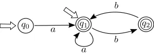
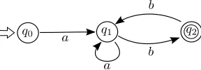
Figure 2 shows an example of a B¨uchi automaton. The initial states are pointed to with large ingoing arrows, and the accepting states are marked with double circles. The automaton in Figure 2, has q0 andq1 as initial states, andq1 and
q2 as accepting states.
The language accepted by a B¨uchi automaton can easily be described in terms of finitary regular languages.
Definition 2.13. LetL ⊆Σ∗ be a set of finite words. We define
Lω:={x
Figure 2: A B¨uchi automaton
Proposition 2.14 (B¨uchi). LetAbe a B¨uchi automaton with initial statesI
and accepting statesF. The languageL(A) accepted byAis precisely
[
qI∈I
[
qF∈F
[qI ։qF]◦[qF ։qF]ω
Proof. An infinite word uis accepted byA if and only if there is anu-labeled successful trace which starts in an initial state qI ∈ I. However, a trace
(qIq1q2. . . , u) is successful if and only if there is some stateqF ∈F such that
qi=qF for infinitely many i∈ω. From this the result follows easily.
The second condition is a bit more involved. If Q is the set of states of some automaton and n is some natural number, we call a function p: Q → {1,2, . . . , n} aparity map.
Definition 2.15(Parity automata). LetAbe an automaton with statesQand acceptance conditionAcc. We say thatAcc is aparity acceptance condition and Ais aparity automaton if there is a parity map p:Q→ {1,2, . . . , n} such that
Acc={X ⊆Q|max(p[X]) is even}.
In other words, a traceτthrough an automatonAwith parity mappis successful if and only if the element of inf(τ) with highest parity is even.
Both of these conditions are useful because the success of a trace is witnessed by a single state in its infinite behavior; a fact which makes reasoning about these sort of automata much easier. Surpringly, by the next theorem we can al-ways assume our automata to be of this kind, and in the case of parity automata, we can also assume the underlying transition system to be deterministic.
Definition 2.16. An automaton A is said to be deterministic if the set I of initial states is a singleton set and for every q∈Q, a∈Σ, there isexactly one
q′ ∈Qsuch thatq→a q′ inA.
Theorem 2.17. LetL ⊆Σω be a set of infinite words. Then the following are
equivalent:
(a) Lisω-regular, i.e.,Lis accepted by an automaton.
(b) Lis accepted by a (possibly non-deterministic) B¨uchi automaton.
(c) Lis accepted by a deterministic parity automaton.
Using the (a)⇒(b) part of the theorem, we get the following characterization theorem for regular languages.
Theorem 2.18 (B¨uchi). A language L is ω-regular if and only if there is a finite set{X0, Y0, X1, Y1, . . . , Xn−1, Yn−1}of regular languages such that
L=[
i<n
Xi◦Yiω
Proof. IfLis regular, then by Theorem 2.17 there is a B¨uchi automaton which accepts L. The result then follows from Proposition 2.14.
We omit the proof of the other direction, since a similar construction is used when proving the analogous Theorem 5.3.
Note that if A is a deterministic automaton whose single initial state is
qI, then, for every infinite wordu, there is exactly one u-labeled trace which
starts in qI. Since B¨uchi automata are the simplest to work with, we would
have hoped that deterministic B¨uchi automata would suffice, but unfortunately there are ω-regular languages which are not accepted by deterministic B¨uchi automata. However, there is another class of automata which almost do the trick, and which also correspond to the “syntactic” automata for finitary regular languages, namely prophetic automata.
2.3
Prophetic automata
Definition 2.19. An automaton Ais said to beprophetic if for every infinite wordu, there isexactly one successfulu-labeled trace throughA.
Now, if we assume that our automata are trim1, meaning that for every
stateq, the languageLω(q) is non-empty, we get the following proposition.
Proposition 2.20. LetAbe an automaton. ThenAis prophetic if and only if
[
q∈A
Lω(q) = Σω (1)
and
Lω(q)∩ Lω(q′) =∅for all distinctq, q′∈A. (2)
In other words, Ais prophetic if and only if the setsLω(q) form apartition of
Σω.
Notice the almost deterministic quality of prophetic automata. As long as we are only interested insuccessfultraces, there is but one choice. It is therefore quite surprising that the class of prophetic B¨uchi automata is equally strong in expressive power as the class of all automata.
Theorem 2.21 (Carton & Michel). For everyω-regular languageL, there is a prophetic B¨uchi automatonAwhich acceptsL.
1It should be fairly clear that this is safe to assume since every state which defines the
Proof. This was proven in [12] where the term “complete and unambiguous” is used instead of “prophetic”, the latter borrowed from [15].
3
(Sourced) Flows
This chapter defines the primary objects of our investigation, namely sourced flows. These can be seen in two ways; as a natural coalgebraic generalization of an infinite word, or as the natural class of structures for which the modal
µ-calculus of one modal “next”-operator applies.
Definition 3.1. A flow S consists of a non-empty set S, called the carrier ofS, together with a functionσ:S→Σ×S called thetransition function or successor function ofS. Elements ofSare usually designated with lettersr, s, t, and are called thestates of (orpoints in)S. Ifσ(s) = (a, s′) we callathecolor ofsands′ thesuccessor ofs.
[image:13.595.156.438.342.431.2]Alternatively, we can think of flows as the special case of a labeled transition system in which each point has a unique successor, i.e., for every states there is a unique pair (a, s′) ∈Σ×S such that s−→a s′. This point of view will be very helpful to us later when we consider automata operating on flows, since it enables us to see the structural similarities between the two classes of objects.
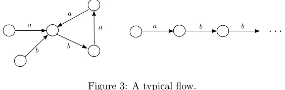
Figure 3: A typical flow.
Figure 3 shows a typical flow over the alphabet{a, b}. Note that it is not connected being the disjoint union of two flows. Another illustrative example is the two way infinite flow
. . .→ −2a → −1b →a 0→b 1→a 2→b . . .
showing that it is quite possible for every point to have a predecessor.
Since flows can be seen as a special case of labeled transition systems, we adopt the same notation.
Definition 3.2. LetS be a flow. We writes→a s′ forϕ(s) = (a, s′) ands։x s′
if and only if either
• x=ǫands=s′, or
• x=ax′ and there is ans′′∈S such thats→a s′′ ands′′։x′ s′.
The objects satisfying formulas of the modalµ-calculus of one modal “next”-operator are points in flows, or alternatively, pointed flows, i.e., pairs (S, s), where s is a point in S. However, in this thesis, it will be very convenient to restrict our attention to pointed flows of a certain kind, namely those where the flow isgenerated by the designated point.
Definition 3.3. LetS = (S, σ) be a flow and lets∈ S. The flowSs= (Ss, σs)
is defined by letting Ss ={s′ | ∃x s x
is the subflow of S generated bys. IfS =Ssfor some s∈ S, we say thatS is
point-generated (bys).
Definition 3.4. Asourced flow Sis a structure (S, s), whereS is generated by
s, i.e., S=Ss. We callsthesource ofS.
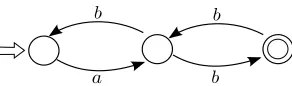
One might think that since the underlying flow is generated by the source, the extra mention of s is superfluous. The reason why we need to explicitely mention it is that a point which generates a point-generated flow need not be unique. For instance, the flowS in Figure 4 is generated by each of its points.
Figure 4: A flow with several generators.
It is well-known that if (S, s) is a pointed flow andϕis a modalµ-calculus formula, then ϕ is true for (S, s) if and only ifϕ is true for (Ss, s). So, our
restriction to sourced flows as opposed to pointed flows does not cause any loss in information in this sense.
3.1
The coalgebraic perspective
As can be seen from its definition, a flow is a coalgebra over the functor Σ×id (see Appendix A for a brief introduction to universal coalgebra). The benefit of having this perspective is that it enables us to use the standard toolkit of universal coalgebra in our arguments. We have already seen one of these tools, namely the definition of a generated subflow above. This, together with the following definitions of homomorphism, bisimulation, final flow and behavioral equivalence are precisely what the definitions from universal coalgebra boil down to if spelled out for our specific functor Σ×id .
First, to simplify notation, ifSandT are flows, we will often writef:S → T for a function between thecarriers ofS toT, and similarily for relations. The same applies to sourced flows, in the sense that if S= (Ss, s) andT = (Tt, t),
we writef:S→Tfor a function between the carriers of theSsand Tt.
Definition 3.5. Let S and T be two flows. A function f: S → T is a ho-momorphism from S to T if s →a s′ in S implies f(s) →a f(s′) in T for all
s, s′∈S.
Forsourced flows, we also require that the functionf maps initial points to initial points. I.e., if S = (Ss, s) and T = (Tt, t) are two sourced flows, then
f:S→Tis a homomorphism if and only if it is a homomorphism from S toT such thatf(s) =t.
Note that in the absence of multiple successors, the “back” condition which occurs when defining bounded morphisms in the setting of Kripke frames be-comes superfluous. For the same reason, the definition of a bisimulation simpli-fies to the following.
Letsandtbe points in two flowsS andT, respectively. We say thatsand
t arebisimilar , if there exists a bisimulationR⊆ S × T such that (s, t)∈R. We now lift this relation on points of flows to sourced flows by saying that two sourced flows (Ss, s) and (Tt, t) are bisimilar, written (Ss, s)↔(Tt, t), if s
andt are bisimilar.
The primary aim of this thesis will be to define acceptance of a sourced flow by an automaton. We get our inspiration from the fact that infinite words can themselves be seen as a special case of sourced flows, namely the infinite ones.
3.2
Infinite words as sourced flows
An infinite worduis a function fromω to Σ, and can thus be seen as acoloring of the setω. However, in our case, the essential point of the matter is thatωcan be seen as atransition structurewith an initial point (namely 0) and where each element has a unique successor. Indeed, weidentify an infinite wordu: ω→Σ with the sourced flow whose carrier is the setω, where the transition function isλi.(u(i), i+ 1) and where the initial point is 0.
0u→(0)1u→(1)2u→(2). . .
Seen through this perspective, the infinite words have a special place amongst the pointed flows as seen by the following two propositions.
Proposition 3.7. Two infinite wordsuandv are bisimilar if and only if they are identical.
Proof. By simple induction using the definition of bisimilarity in the successor steps.
Proposition 3.8. For every sourced flowSthere is a unique bisimilar infinite word−→S, called the unraveling of S. In fact, there is a unique homomorphism
US:
− →
S →S.
The “U” in the above proposition is for “unravel”, although, strictly speak-ing, the unraveling is in the other direction. See Figure 5.
Proof. Let S = (Ss0, s0) be a sourced flow. We inductively create a sequence
s0s1. . . of states ofS and a sequencea0a1. . . of symbols of Σ by settingai and
si+1 to be the unique pair such thatsi ai
→si+1 (note thats0is already given).
The unraveling −→S ofSis the infinite worda0a1. . ., i.e.,
0 a0 →1 a1
→2 a2 →. . .
and the homomorphism is quite simply the sequence s0s1. . . when seen as a
function fromω toS.
The uniqueness ofa0a1. . . follows from the preceding proposition and the
uniqueness of the homomorphism follows from the fact thatanyhomomorphism
Figure 5: Unwinding a sourced flowS
From this we obtain a simple way of checking whether two sourced flows are bisimilar.
Corollary 3.9. Two sourced flowsSandTare bisimilar if and only if−→S =−→T.
Proof. Assume thatS andTare bisimilar. It is easy to check that bisimilarity is a transitive relation over sourced flows, and hence−→S and−→T are bisimilar as well. But then−→S =−→T. The other direction is similarily straight forward.
In fact, there is another way to view the unraveling of a pointed flow S with initial point s, namely as the behavior of s. The notion of behavioral equivalence is a fairly abstract notion (see Appendix A), but in our case it becomes simplified, since the category of flows has afinal object.
Fact 3.10. We writeΣωfor the flow whose elements are infinite wordsu∈Σω
and where the transition function is defined asau→a ufor alla∈Σ,u∈Σω.
The flowΣω is final in the category of all flows, i.e., for every flowS there is a unique homomorphism !S: S →Σω, which is defined by
!S(s) =
−−−−→ (Ss, s).
We say that two pointed flows (S, s) and (T, t) arebehaviorally equivalent if !S(s) =!T(t). However, this is equivalent to saying that
−−−−→ (Ss, s) =
−−−→ (Tt, t) which
in turn is equivalent to saying that the two sourced flows (Ss, s) and (Tt, t) are
bisimilar.
It is easy to see that a source-pointed flowSis infinite (has an infinite carrier) if and only if it is (isomorphic to) an infinite word. Now, since one of the aims of our thesis is to come up with a natural definition of an automaton accepting a sourced flow, and we already know how to deal with infinite words, we are more interested in thefinite sourced flows. These are the ones in which the successor function eventually loops. If we go back again to the modal µ-calculus, these can be seen as the finite models of the logic and are therefore interesting in their own right.
3.3
Lassos
Definition 3.11. A finite sourced flowS= (Ss, s) (i.e., where the carrier ofSs
is finite) is called alasso. The least subset ofSswhich is closed under successor
We give a special name to the point of the loop which is closest to the source.
Definition 3.12. LetS be a sourced flow with sources. For each pointtofS we say thatd(s) = min{|x| |s։x t}is thedistance from the source tot.
[image:17.595.210.385.225.290.2]Definition 3.13. If S is a lasso with sources, we call the pointt of the loop with the least distance fromstheknot point ofS.
Figure 6: A lasso showing its parts.
LetS be a lasso with source s and knot pointr. Letxbe the least string such that s։x r and lety be the least string such thatr։y r. It is easy to see that −→S =xyω and that xand y uniquely determine S up to isomorphism, in
the sense that the lasso (x, y) defined below will be isomorphic toS.
Definition 3.14. Given finite strings xand y, wherey is nonempty, we write (x, y) for the lasso whose carrier is the set{0,1, . . . ,|xy|−1}; where the transition functionσis defined by
σ(i) =
(x(i), i+ 1) ifi <|x|,
(y(i), i+ 1) if|x| ≤i <|xy| −1,
(y(i),|x|) ifi=|xy| −1;
[image:17.595.143.448.416.662.2]and where the source is 0. For an example, see figure 7.
Figure 7: The lasso (aba, ab).
Figure 8: Two bisimilar but non-isomorphic lassos.
that this is a name conflict, but we will try to be clear so as to not cause any confusion.
By Corollary 3.9 we know that two lassos (x, y) and (z, w) are bisimilar if and only ifxyω=zwω. However, we could still havex6=z orw6=y. For instance,
4
Automata on flows
We are now ready to define what it means for an automaton to accept an arbi-trary sourced flowS. There are some requirements that we want this definition to satisfy. We want it to be conservative with regards to infinite words (seen as sourced flows) and we want it to bebisimulation invariant, i.e., ifSand Tare bisimilar, then an automatonAshould acceptSif and only if it acceptsT. The second requirement is to guarantee that we keep the equivalence in expressive power between automata and the modal fixed point logic when expanding from infinite words to the set of all flows. These two requirements also makes our definition conform with the general one in [22], although ours is different in that is does not usegamesto define acceptance, instead using homomorphisms and label-preserving maps. There are two primary reasons for this. One is that it enables us to give a definition of acceptance which for finite sourced flows is purely finitary, i.e., it does not need infinite objects as witnesses for acceptance. Secondly, using maps and homomorphisms allow us to see structural similarities between the automata and the sourced flows it accepts, giving us more control when pursuing our goal of finding characterization theorems.
4.1
Traces and runs
The idea of our definition is taken from the game theoretic semantics given in [22] and goes as follows. Take an automatonAand a sourced flowS. We want to stepwise identify states inS with states ofA in a label-preserving way. So, starting by settings0to be the source ofS, we pick some elementq0ofA. Next,
we have that s0 →a0 s1 for some a0 ∈ Σ, s1 ∈ S. We then pick some element
q1∈Asuch thatq0→a0 q1. Continuing in this fashion, we obtain a sequence
(s0, q0, a0),(s1, q1, a1),(s2, q2, a2), . . . (3)
such that si →ai si+1 andqi →ai qi+1 holds for all i∈ ω. In the game theoretic
perspective, this sequence is often called aplay or amatch. Now, if we rewrite the sequence in (3) as
(q0, s0,0)→a0 (q1, s1,1)→a1 (q2, s2,2)→ · · ·a2
we see that this is in fact a sourced flow, which we will designateR. The accute reader might notice that it is isomorphic to the infinite word a0a1. . . which is
also the unraveling of the sourced flow S. This, however, is a bit outside the point (although it will become important later on). The main observation is that the following two statements hold:
• The functionρ: R→Asending a state (qn, sn, n) toqnislabel-preserving
in the sense that ifr→a r′ inR, thenρ(r)→a ρ(r′) inA.
• The function h:R → S sending a state (qn, sn, n) to sn is a
homomor-phism.
Hence, this “stepwise” identification of states yielded the following situation.
R
ρ
h
? ? ? ? ? ? ?
A S
Notice how this diagram is similar, but not identical, to the general coalgebraic notion of a bisimulation. The difference is that the automatonAis not a sourced flow andρis not a homomorphism (and could not reasonably be required to be one, since the automaton Ahas a different coalgebraic signature).
We now use the diagram in (4) to give us our definition of arun, beginning by giving the function ρa special name.
Definition 4.1. LetAbe an automaton andSbe a sourced flow. We say that a functionτ:S→Ais anS-labeledtrace throughAif
s→a s′ =⇒ τ(s)→a τ(s′)
for alls, s′ ∈S,a∈Σ.
Definition 4.2. LetAbe an automaton andSa sourced flow. A run ofA on Sis a traceρ:R→Atogether with a homomorphismh:R→S.
Note that any homomorphism between two sourced flows must be unique if it exists, since it maps the source of the first to the source of the other, and successor points to successor points. So, in the definition above, the actual nature of the homomorphismhdoes not matter, as long as it exists. Hence, as a convention, we will instead say “letρ:R→Abe a run ofAonS”, implying that Ris a homomorphic preimage ofS. Often (but not always), we will make a typographical distinction and write ρ for traces which are also runs, and τ
otherwise.
To determine whether a runρofAon a sourced flowSis accepting or not, we need to look at theinfinite behavior ofρ, when seen as a trace. Recall that in the case for infinite words, acceptance was determined by looking at the set of states of the automaton that were was visited infinitely many times during the run. In our generalized case, this definition won’t do as it stands, but we can reformulate it in such a way that it applies. Instead of asking “which states of the automaton gets mapped to infinitely often byρ”, we ask ourselves “which states q of the automaton are such that wherever you start in the run,q will eventually show up”. Formalizing this gives us the following definition.
Definition 4.3. Letτ:S→Abe a trace. For eachs∈S, letSs be the set of
all pointss′ ∈Ssuch that s։x s′ for somex∈Σ∗. Theinfinite behavior ofτ, inf(τ), is then defined by
inf(τ) :=\
s∈S
τ[Ss].
The definition of whether a trace is successful (accepting) or not becomes the same as the one we saw for infinite words in Definition 2.9.
Definition 4.4. A trace τ:S→Ais said to besuccessful if inf(τ)∈AccA. It
is called accepting if it is successful and starts in an initial point ofA, i.e., if
τ(s0)∈IA, wheres0 is the source ofS.
Definition 4.5. Let A be an automaton. We say that a sourced flow S is accepted by a pointqin Aif there is a successful runρofA onSwhich starts in q. We writeL(q,A) (or simplyL(q), if the automatonAis implicit) for the set of all sourced flows accepted by q.
Similarily, we say thatS isaccepted byAif there is an accepting runρofA onS. We writeL(A) for the set of all sourced flows accepted byA.
For an automatonAwith initial statesI, we immediately get that
L(A) = [
qI∈I
L(qI).
We now show that the definition yields the results we want, namely being conservative with regards to the standard definition over the set of infinite words; being bisimulation invariant; and giving a finitary definition of acceptance for finite sourced flows.
Proposition 4.6. A automatonAaccepts the coalgebraic representation of an infinite wordu(in the sense of Definition 4.5) if and only if it accepts the infinite worduin the ordinary sense (i.e., in the sense of Definition 2.10).
Proof. The result follows from a simple comparison of the two definitions, to-gether with the observation that for infinite sourced flows, Definition 4.3 reduces to the ordinary notion of “infinite behavior”.
Now, in order to prove that the language accepted by an automaton is closed under bisimilarity, we prove the following statement.
Proposition 4.7. Letρ: R→Abe a run of an automatonAon a sourced flow Sand letf be a homomorphism from some sourced flowTtoR. Thenτ =ρ◦f
is a also a run ofAonS. Moreover, τ is successful (accepting) if and only ifρ
is successful (accepting).
T
τ=ρ◦f
h◦f
? ? ? ? ? ? ? f
Aoo ρ R
h
/
[image:21.595.255.339.519.570.2]/S
Figure 9: Runs are preserved by taking homomorphic preimages.
Proof. Sinceρis a run ofAonS, we know thatRis a homomorphic preimage of S, i.e., there is a homomorphism h:R → S. It is easy to check that the composition of two homomorphisms is still a homomorphism, and hence T is a homomorphic preimage of S, using the homomorphismh◦f. Furthermore, it is easy to see that τ = ρ◦f is a trace, since it is the composition of two label-preserving functions.
homomorphism and hence must map successor points to successor points. Our second observation is that f must be surjective. This again follows from the fact that it maps successors to successors, but now combined with the fact that it also is required to map the source ofTto the source ofS. But then we must have
inf(τ) =\
t∈T
τ[Tt]
=\
t∈T
(ρ◦f)[Tt]
=\
t∈T
ρ[f[Tt]]
=\
t∈T
ρ[Rf(t)]
= \
r∈R
ρ[Rr]
= inf(ρ).
Now, since the success of a run is determined in terms of its infinite behavior this means thatτ is successful if and only ifρis. To realize thatτ is accepting if and only if ρis, it is enough to observe that if t0 and r0 are the sources of
T and R, respectively, then τ(t0) =ρ(f(t0)) = ρ(r0). This is because f is a
homomorphism, and therefore, by definition, must map the source of Tto the source ofR.
Corollary 4.8. LetA be an automaton and S a sourced flow. Then the fol-lowing are equivalent:
(a) Sis accepted byA.
(b) −→S is accepted by A
(c) There is an−→S-labeled accepting trace throughA.
Proof. (a)⇒(c). Assume thatAacceptsS. Then there is some runρ:R→A of A on S. But then, according to Proposition 4.7, the function −→ρ: −→R → A defined by −→ρ :=ρ◦UR is an accepting run of A onS. We then have that
− →
R andSare bisimilar, since−→R is a homomorphic preimage ofS. This means that −
→
R =−→S, which means that−→ρ is an−→S-labeled accepting trace. −
→ R =−→S
− →ρ=ρ◦U
R { { xxxx xxxx x UR
h◦UR=US
" " F F F F F F F F F
Aoo ρ R h //S (c)⇒(b). Immediate.
Proposition 4.9. If S and Tare two bisimilar sourced flows and Ais an au-tomaton, thenAacceptsS if and only ifAacceptsT.
Proof. We know that S andT are bisimilar if and only if−→S =−→T. The result then follows from Corollary 4.8.
Having shown that our definition behaves nicely with respect to infinite words and bisimulation, we are now ready to show our last claim, namely that for lassos, the definition can be made purely finitary. We will do this by defining thefinitary fragment of a regular language of sourced flows, and looking at its properties. First, we introduce a special subset of the language accepted by an automaton, namely those sourced flows which are the domain of an accepting trace, as they will play an important part in the rest of the thesis.
4.2
Labels
In Proposition 4.8, we saw that an automaton A accepts a sourced flow S if and only if there is an accepting trace ρ:−→S →A. Hence, if S is infinite, i.e., ifS=−→S, then there is an accepting trace ρwhose label isS. The reason why these are to become important is that the traceρwill enable us to reason about similarities in structure betweenAandS.
Definition 4.10. LetAbe an automaton andqa state inA. IfSis the label of a successful trace throughAwhich starts inq, i.e., if there is a successful trace
ρ:S→A, we say thatSis asuccessful label ofq. The set of successful labels of
qis denoted Label(q,A), or simply Label(q) if the automatonAis implicit. Similarily, we call S anaccepting label of Aif it is a successful label of an initial point of A, i.e., if there exists an accepting trace ρ:S → A. We write Label(A) for the set of accepting labels ofA.
Using this definition, we obtain the following proposition which is just a reformulation of Definition 4.5.
Proposition 4.11. The language L(A) accepted by an automaton A is the closure of the set Label(A) under homomorphic images.
Since Label(A) is closed under homomorphic preimages, it is not difficult to see that this is equivalent to saying thatL(A) is the closure of Label(A) under bisimilarity.
If we letAbe the automaton displayed in Figure 10, we get an example of when the two languagesL(A) and Label(A) don’t coincide. To see why, consider the lasso (a, b). Certainly the infinite word abω is accepted by A, so the lasso
(a, b) is as well. However, there areno(a, b)-labeled traces throughAas can be realized by asking which state of Athe single point in the loop of (a, b) would be mapped to. In a sense, the righthand “loop” inAis too big. In Section 4.4 of this chapter, we will see that forprophetic automata, the two languages always coincide.
4.3
Regular lasso languages
Figure 10: An example of when Label(A)6=L(A)
µ-calculus of one modal operator. Hence, by studying these in particular, we are doingfinite model theory for this logic.
Recalling how we defined Lasso to be the set of finite sourced flows, and Streamas the set of infinite ones, we define the finitary and infinitary fragments of a language of sourced flows in the following way.
Definition 4.12. IfLis a language of sourced flows, we define
Lfin :=L ∩Lasso
Lω:=L ∩Stream.
These are respectively called the finitary and infinitary fragments of the lan-guage L.
Proposition 4.13. The class of regular languages of sourced flows is closed under intersection, union and complementation.
Proof. This follows from the fact that the statement holds for the infinitary fragments. As an example we show closure under intersection.
LetL andL′ be two regular languages of sourced flows. Consider the sets
Lω andL′ω of infinite sourced flows,seen as sets of infinite words. Then both
Lω and L′ω are ω-regular languages, and since ω-regular languages are closed
under intersection, we have thatLω∩ L′ωisω-regular. But then the automaton
which acceptsLω∩ L′ω also acceptsL ∩ L′, sinceL ∩ L′is the closure ofLω∩ L′ω
under homomorphic images.
From this we obtain the well-known result (although rephrased in our ter-minology) that regular languages are determined by their finitary fragment.
Theorem 4.14. Let L,L′ be regular languages of sourced flows. Then the
following are equivalent:
(a) L=L′
(b) Lω=L′ω
(c) Lfin=L′fin
Proof. That (a)⇒(b) is clear. For the case of (b)⇒(c), ifL′
fin6=L′fin, we can,
without loss of generality, assume that there is some lassoS∈ L \ L′. But then
− →
S ∈ L \ L′, since bothLandL′are closed under bisimilarity. Hence,L
ω6=L′ω.
To prove that (c)⇒(a), assume thatL 6=L′. Without loss of generality, we
can assume thatL \ L′ is non-empty, and we want to show thatL \ L′ contains
some lasso, from which the result follows.
which accepts it. Now, sinceAis finite and acceptssome sourced flowS(since we assumed thatL \ L′ was non-empty), it is not difficult to see that there must
be some finite path from an initial point qI to some accepting point qF (say
with labelx), and a non-empty finite path fromqF back to itself (say with label
y). But then the lasso (x, y) is an element ofL \ L′.
We define the following shorthands for the finitary fragments of the languages defined by an automatonA.
Definition 4.15. LetAbe an automaton. We define
Labelfin(q,A) := Label(q,A)∩Lasso
Labelfin(A) := Label(A)∩Lasso
Lfin(q,A) :=L(q,A)∩Lasso
Lfin(A) :=L(A)∩Lasso
The languageLAis called thefinitary language, or lasso language, accepted
by A. We say that a languageLof lassos is aregular lasso language if there is an automaton Asuch thatL is the lasso language accepted byA.
What we want is a purely finitary definition of a regular lasso-language, since these correspond to the definable classes of finitary models in the modal
µ-calculus. As we saw in Proposition 4.11, the language accepted by Ais the closure of Label(A) under homomorphic images. For a finitary version of this, we would like the lasso-languageLfin(A) accepted by an automatonAto be the
closure of Labelfin(A) under homomorphic images. Calling a runρ:R→Aon a
sourced flowSfinite ifRis finite, this is equivalent to requiring that whenever there exists an infinite accepting run ρof an automaton Aon afinite sourced flowS, then there also exists afinite runρ′ ofAonS.
In fact, we can do even better, as we can give a bound on how “big” the run has to be, in terms of the size of the automaton.
Theorem 4.16. LetAbe an automaton withkstates and let (x, y) be a lasso inL(A). Then there aren < k+k3andm < k3, dependent on (x, y), such that
(xyn, ym)∈Label
fin(A).
These upper bounds are probably not optimal, since there is much room for “tweaking” the proof in order to obtain better results.
Proof. Assume thatAhaskstates and that (x, y)∈ L(A). Then there must be an accepting traceτ throughAwhose label is the infinite wordxyω. We show
that we can assume thatτ is of a certain form, which will enable us to create a finite accepting trace with the required properties.
Our infinite trace τ consists of a label preserving function from the flow representation of the infinite word xyω. Writing x(i) for the i:th symbol of x
(indexing from zero), and similarily fory, we have a sequence of statesq0, q1, . . .
of the automaton such that
q0
x(0)
→ q1
x(1)
→ . . .x(|x→|−1)q|x|
y(0)
→ q|x|+1
y(1)
→ . . .y(|y→|−1)q|x|+|y|
y(0)
We are especially interested in the statesq|x|+|y|·i for different values ofi∈ω,
so we writeqi:=q
|x|+|y|·i and can then write the trace above as
q0
x
։q0։y q1։y . . .
Sinceτ is accepting, there is a setF ∈AccAsuch that inf(τ) =F. This means
that after some point in the sequenceq0, q1, . . ., only elements of F occurs. So
we can letm0 be the least natural number such that
{τ(i)|i≥ |x|+|y| ·m0}=F.
Now, if we start at some point qi where i is greater than |x|+|y| ·m0, then
there must be somej ≥isuch that{qi, qi+1, . . . , qj}=F. Moreover, for every
j′ greater thanj,{q
i, qi+1, . . . , qj′}is equal toF as well. Writing [qi, qj] for the inclusive interval between the pointsqi andqj, i.e.,
[qi, qj] :={q
n| |x|+|y| ·i≤n≤ |x|+|y| ·j}
we can therefore inductively definemi+1to be the least such that [qmi, qmi+1] =
F. Then, if we consider the traceτ up toqmk,
q0
xym
0 ։ qm0 y
m1−m0 ։ qm1 y
m2−m1 ։ qm1y
m3−m2 ։ · · ·y
mk−mk−1 ։ qmk,
at least two of the points in the set {qm0, qm1, . . . , qmk}must be identical, i.e., there area < b≤ksuch that qma =qmb. But this means that we have found
a “loop” in the automaton, by which we mean that the string ymb−ma is the label of a finite path fromqma back to itself. Now, by construction, this finite
path passes through every element ofF. So, moving first by from q0 toqma by
means of the finitexyma-labeled pathq
0, q1, . . . , qmaand then back fromqmato
itself by means of theymb−ma-labeled path we just found, gives us an accepting
trace whose label is (xyma, ymb−ma).
Finally, we show that we can assume that m0 < k and mk −m0 < k3,
concluding our proof. For the first statement, observe the trace up to qm0:
q0
x
։q0։y q1։y q2։y · · ·։y qm0
Ifm0≥k, then two of the states in the set{q0, q1, . . . , qm0}must be equal, and
hence we can remove the segment between these two points without changing the label or the acceptance of the trace. Hence, it is safe to assume thatm0< k.
For the second statement, we prove that for everyi < k,mi+1−mi can be
assumed to be less thank2. This suffices because thenm
k−m0= (m1−m0) +
(m2−m1) +. . .+ (mk−mk−1)< k3.
Consider the trace betweenqmi andqmi+1 for some choice ofi:
qmi ։y qmi+1։y · · ·։y qmi+1−1։y qmi+1
The idea is that this path must “accumulate” states fromF one by one, allowing us to split it into subpaths which we then show can be assumed to be bounded in length. We start by letting l0 = mi and inductively setting lj+1 to be the
least natural number≥lj such that
In other words, we start at ql0, move stepwise through the trace, and increase the “counter” variable j each time we are at a point qn (for some n), having
encountered an element ofF which we haven’t seen before. Now, since we start by having “seen”ql0, the counter variablej can only increase to some number
h < k. In other words, we know that the sizes of the sets
[ql0, ql0]([ql0, ql1](· · ·([ql0, qlh]
are strictly increasing, but are bounded by |F| ≤ k. By our choice ofmi+1 we
must have a situation which looks like this:
qmi =ql0y
l1−l0 ։ ql1y
l2−l1 ։ ql2y
l3−l2 ։ · · ·y
lh−lh−1 ։ qlh
| {z }
≤kintervals
=qmi+1
The final step is now to give a bound forlj+1−lj. Consider the segment of the
trace between the pointsqlj andqlj+1:
qlj ։y qlj+1։y · · ·։y qlj+1−1
| {z }
no new points ofFhere
y
։qlj+1
Certainly, iflj+1−lj≥k, then the set{qlj, qlj+1, . . . , qlj+1}would have more
thankelements. Therefore we should be able to reason as in the case ofm0, and
remove the segment of the trace between these two points. However, in doing so we might accidentally remove a point such that the interval [qmi, qmi+1] no longer contains every element of F. Luckily, the minimality of lj+1 guarantees that
[qmi, qlj] = [qmi, qmj+1−1], so removing segments in the interval [qlj, qlj+1−1] is safe. So, we can argue as follows: if lj+1−lj is strictly greater than k, then
the set {qlj, qlj+1, . . . , qlj+1−1} has cardinality greater than k and hence there are two points which are equal. By the above discussion, removing the segment between these two points does not alter the label of the trace, nor the fact that [qmi, qmi+1] =F. Hence, we may safely assume thatl
j+1−lj ≤k. But then
mi+1−mi= j=h−1
X
j=0
(lj+1−lj)
≤
j=h−1 X
j=0
k
< k2,
as required.
Having these upper bounds enables us to give auniform size for the wit-nessing lasso in Label(A).
Corollary 4.17. LetAbe an automaton withkstates. Then
(x, y)∈ L(A) ⇐⇒ (xyk+k3, yk3!)∈Label(A).
Proof. The main observation to make here is that if we takex∈Σ∗, y ∈Σ+,
n ≥0, m ≥1, and consider the lasso (xyn, ym), then for any n′ ≥n and any
multiplem′ ofm, (xyn, ym) is a homomorphic image of (xyn′
Hence, the direction from right to left is immediate, since (x, y) is a homo-morphic image of (xyk+k3
, yk3
!). For the other direction, assume that (x, y) is
ac-cepted byA. Then there aren < k+k3, m < k3such that (xyn, ym)∈Label(A).
By choosingn′=k+k3andm′ =k3!, we getn′ > nand that m′ is a multiple ofm; hence we obtain the wanted result.
We also get the result we want, namely that a finite sourced flowSis accepted by an automatonAif and only if there is afinite run ρ:R→AofAonS.
Corollary 4.18. IfAis an automaton, thenLfin(A) is the closure of Labelfin(A)
under homomorphic images.
Since Labelfin(A) is closed under homomorphic preimages, restricted to the
set of lassos, it is not difficult to check that Lfin(A) is also the closure of
Labelfin(A) under bisimilarity, restricted to the set of lassos. This can also
be realized by noting that Lfin(A)must be closed under bisimilarity restricted
to the set of lassos, sinceL(A) is closed under bisimilarity over the entire class of sourced flows.
4.4
Prophetic automata and labels
As we have seen, it is not in general the case that the set Label(A) of accepting labels of an automaton A coincides with the set of accepted sourced flows. It turns out that the set Label(A) is easier to investigate than L(A), because of the similarities in structure between the lassos in Label(A) and the automaton Aitself.
Here we show that for aprophetic B¨uchi automatonA, as defined in section 2.3, the two sets L(A) and Label(A) are equal. In fact, we get a stronger property, namely that the sets Label(q) for each q∈A, constitutes a partition of the class of all pointed flows, where each class is closed under bisimulation.
Theorem 4.19. LetAbe a B¨uchi automaton. ThenAis prophetic if and only if for every sourced flowS, there is a unique successful traceτ: S→A.
Proof. Note that an automaton is prophetic if and only if this theorem holds when restricted to the class of infinite words, i.e., the infinite sourced flows. Hence, the direction from right to left is immediate.
For the direction from left to right, assume that Ais prophetic. Then, for every infinite word uthere is a unique successful trace τu:u→ A(remember
that we identify infinite words with their sourced flow representation).
Now, take an arbitrary sourced flowSand letu=−→S be its unraveling. We know that there is a unique homomorphismUS:u→S, and by proposition 4.7,
we know that if there is a successful trace
τ:S→A,
then
τ◦ US:u→A
is a successful trace as well. By the uniqueness of τu, this would imply that
τu=τ◦US, and hence there is really just one choice forτ, namely the function
which maps a state s∈S to the unique stateq ∈Asuch that ifUS(i) =s for
So, it suffices to show that if i, j ∈ −→S are such that US(i) = US(j), then
τ(i) =τ(j). However, ifUS(i) =US(j), then the pointsiandjare behaviorally
equivalent, and hence the suffixes of ugenerated by i and j, respectively, are identical.
0 a0 →1 a1
→. . .ai−1
→ i→ai i+ 1ai+1
→ . . .aj→−1j→aj j+ 1aj+1 → . . .
Because of the uniqueness of the successful traces, if v ∈ Σω is a suffix of u,
thenτv must conform withτu, i.e.,τv=τu↾v. Hence,τ(i) =τ(j).
From this we obtain a corollary which is analoguous to Proposition 2.20.
Corollary 4.20. An automatonAis prophetic if and only if{Label(q)|q∈A} partitionsSFlow.
We also obtain the result which was mentioned in the beginning of this subsection, namely that for prophetic automata A, Label(A) is closed under bisimilarity. This is implied by the following corollary.
Corollary 4.21. If A is prophetic, then Label(q) is closed under bisimilarity for every q∈A.
Proof. Take a prophetic automatonAand consider two bisimilar sourced flows S andT. There are uniqueq, q′ ∈Asuch thatS∈Label(q) andT∈Label(q′).
Then−→S ∈Label(q) and−→T ∈Label(q′). BecauseSandTare bisimilar, we have
− →
S =−→T and hence we must haveq=q′.
Prophetic automata can be characterized in yet another way, showing a connection to the final flow (the final object in the category of flows). The result will not be used in the rest of the thesis, but is mentioned here anyway since we think it is an interesting result on its own. Let A be an automaton and S be a (non-pointed) flow. We temporarily call a function τ: S → A a successful trace if, for every s∈ S,τ restricted to the sourced flow (Ss, s) is a
successful trace in the ordinary sense.
Theorem 4.22. An automatonAis prophetic if and only if there is surjective successful trace τ: Σω→Awhich is unique with respect to being successful.
5
Characterizating regular lasso languages
Recall from Definition 4.15 that a setL ⊆Lassois called aregular lasso language if it is the lasso fragment of a regular language of pointed flows, i.e., if there is an automaton Asuch thatL=Lfin(A).
Our aim in this section is to look for interesting properties shared by these regular lasso languages, ultimately seeking out those properties which are equiv-alent to regularity.
We will often define sets of lassos by specifying their sets of spokes and loops. For this reason, we introduce the following conveniant shorthand.
Definition 5.1. LetX, Y ⊆Σ∗be sets of finite strings, whereǫ6∈Y. We let
Lassos(X, Y) :={(x, y)|x∈X, y∈Y },
saying that Lassos(X, Y) is the set (or language) of lassosgenerated by X and
Y.
5.1
Characterization using finitary regular languages
Our first characterization theorem is an analogue of Theorem 2.18 of the pre-liminaries in whichω-regular languages were defined in terms of finitary regular languages. To establish a similar result for regular languages of lassos, we first prove an analogue of Proposition 2.14. For this, letA be a B¨uchi automaton, (x, y) be a lasso, and consider a (x, y)-labeled traceτ throughA. Such a trace is accepting if and only if• the initial state of (x, y) to some initial stateqI ofA,
• the knot point of (x, y) to some stateqofA,
• some point of the loop of (x, y) to some accepting stateqF.
In other words, (x, y)∈Labelfin(A) if and only if
qI x
։q։y1 qF y2 ։q
for some qI ∈ IA, q ∈ QA, qF ∈ FA, and y1, y2 ∈ Σ∗ such that y1y2 = y.
Reformulated, we have the following.
Proposition 5.2. LetAbe a B¨uchi automaton. Then
Labelfin(A) = [
qI∈IA
[
q∈A
[
qF∈FA
Lassos ([qI ։q],([q։qF]◦[qF ։q])\ {ǫ})
As a reminder, Theorem 2.18 states that a languageL ⊆Σω isω-regular if
and only if
L=[
i<n
Xi◦Yiω
for some finite set of regular languages{X0, Y0, . . . , Xn−1, Yn−1}. We will prove
the separation of the “loop-part” Y and the “spoke-part”X isn’t as clear cut. What we get instead is the following.
Theorem 5.3. A bisimulation closed set of lassosLis regular if and only if
L= [
i<n
Lassos(XiYi∗, Yi+)
for some finite set {X0, Y0, X1, Y1, . . . , Xn−1, Yn−1} of regular languages (over
Σ∗) such thatY
i does not contain the empty string,ǫ, for any i < n.
The proof from right to left will use the following lemma.
Lemma 5.4. For every pair (X, Y) of regular languages X, Y ⊆ Σ∗ such
that ǫ 6∈ Y, there is an automaton A such that Lfin(A) is the closure of
Lassos(XY∗, Y+) under bisimilarity, restricted to the set of lassos.
This in turn will be proven using two well-known results about regular lan-guages over Σ∗. The same sort of construction can for instance be found in the
proof of Theorem 5.4 in [15], page 28. They are proved here for the sake of completeness.
The first of the lemmas gives us an automaton of a special shape for the “spoke”-part of our lasso language.
Definition 5.5. We call a state q in an automaton A a sink if there are no outgoing transitions fromq, i.e., q→a q′ doesnot hold for anya∈Σ,q′ ∈A.
Lemma 5.6. For every regular language X ⊆Σ∗, there is an automaton A
s
which acceptsX, such thatAshas a single accepting stateqF which is a sink.
Proof. SinceX is a regular language, there is some automaton A= (QA,∆A, IA, FA)
which acceptsX. We construct our automaton
As= (QAs,∆As, IAs, FAs)
by adding a new pointrtoA, setting it as the single accepting point and adding transitions to it from states which used to see an accepting point. More formally, we let
QAs =QA⊎ {r}
IAs =
(
IA ifIA∩FA=∅, i.e.,ǫ6∈ L(A)
IA∪ {r} otherwise.
FAs ={r}
and define the transition function by setting
q→a q′ inAs ⇐⇒
(
q→a q′ in A, or
q′=rand∃q
F ∈FAs.t. q a
→qF inA
Now, it is clear that by construction,Aaccepts the empty word if and only if As accepts it. For the case of a non-empty word x we have that, for an
arbitraryq∈QA, q x
։qF for someqF ∈FAif and only ifq x
։rin As. Hence,
The second lemma gives us an automaton for the “loop”-part.
Lemma 5.7. IfY ⊆Σ∗ is a regular language such thatY =Y∗, then there is
an automatonAlwhich acceptsY such thatAlhas a single initial and accepting
state which coincide, i.e.,IAl =FAl={qF}for someqF ∈Al.
Proof. The proof is similar to the previous one. We take an existing automaton Awith initial states IAand accepting states FA, add a new point rwhich will
be the new single initial and accepting state. Again, we add transitions to r
from those states ofAwhich see an accepting point, but we also add transitions from rto those states ofAwhich areseen by an initial point. Formally, we let Al be an automaton defined by
QAl=QA⊎ {r}
IAl={r}
FAl={r}
and we define the transition function by letting
q→a q′ inAl ⇐⇒
q→a q′ inA, or
q′=rand∃q
F ∈FAs.t. q a
→qF in A, or
q=rand∃qI ∈IAs.t. qI a
→q′ inA, or
q=q′ =rand ∃q
I ∈IA, qF ∈FAs.t. qI a
→qF inA.
It is easy to see thatL(A)⊆ L(Al), since any accepting path
q0→a0 q1→a1 . . .
an−2 → qn−1
an−1 → qn
in Ayields an accepting path
ra0 →q1
a1
→. . .an−2 → qn−1
an−1 → r
in Al. For the other direction, note that for every path in Al which is of the
form
ra0 →q1
a1
→. . .an−2 → qn−1
an−1
→ r (5)
where all of the statesq1, . . . , qn−1are also inA(i.e., are distinct fromr), there
areqI ∈IAandqF ∈FA such that
qI a0 →q1
a1
→. . .an−2 → qn−1
an−1 → qF
is a path in A. Given the requirement that L(A) = Y = Y∗, the result now follows from the observation that any accepting path throughAlmust either be
the empty path or be a concatenation of paths of the form in (5).
Proof of Lemma 5.4. LetX, Y ⊆Σ∗ be regular languages where ǫ6∈Y and let
Lbe the closure of Lassos(XY∗, Y+) under bisimilarity, restricted to the set of
lassos. Our aim is to build an automatonAsuch thatLfin(A) =L.
According to Lemma 5.6 there is an automatonAsacceptingX with a single
accepting stateqF which is a sink. Similarily, Lemma 5.7 provides us with an
automaton As with a single initial and accepting state q′F. We now combine
we let qF =qF′ , thereby identifying the accepting state of As with the initial
and accepting state ofAl. Next, we letAbe the automaton defined by
QA=QAs∪QAl
∆A= ∆As∪∆Al
IA=IAs
FA={qF}.
We now show thatL=Lfin(A) by showing that
(a) Lassos(XY∗, Y+)⊆Labelfin(A); and
(b) for every lasso in Labelfin(A) there is a bisimilar one in Lassos(XY∗, Y+).
This suffices, since then the bisimulation closure of Lassos(XY∗, Y+) is equal to the bisimulation closure of Labelfin(A) (restricted to the set of lassos). But
the former is preciselyLand the latter is preciselyLfin(A).
(a) Consider a lasso (xy, y′) ∈ Lassos(XY∗, Y+) such that x∈ X, y ∈ Y∗
and y′ ∈ Y+. By the construction of our automaton A, x is the label of a finite path from an initial state qI to qF, y is the label of a finite path from
qF to qF andy′ is the label of a non-empty finite path fromqF to qF. Hence
qI xy
։qF y′
։qF. But this means that (xy, y′) is the label of an accepting trace
throughA, i.e., (xy, y′)∈Label
fin(A).
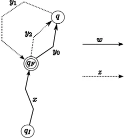
(b) Let (w, z) be a lasso in Labelfin(A). Our aim is to construct a bisimilar
[image:33.595.234.359.427.565.2]lasso (xy, y′) such thatx∈X, y∈Y∗ andy′∈Y+.
Figure 11: Deconstructing a lasso (w, z)∈Labelfin(A)
Keeping Figure 11 in mind, we argue as follows. Since (w, z) is the label of an accepting path throughA, we have that wis the label of a finite path from some initial state qI to some state q and z is the label of a non-empty finite
path fromqback to itself which passes through the accepting stateqF. In other
words, there must bey1, y2∈Σ∗such that z=y1y2 and
qI w
։q։y1 qF y2 ։q.
Our first observation is that all the states in the finite path