A glaciochemical study of the Mill Island ice core

(1)

A GLACIOCHEMICAL STUDY OF THE

MILL ISLAND ICE CORE

by

Mana Inoue, B.Eng, B.AntStd. Hons

Submitted in fulfilment of the requirements for the Degree of Doctor of Philosophy

Institute for Marine and Antarctic Studies

University of Tasmania

(2)

ii

I declare that this thesis contains no material which has been ac-cepted for a degree or diploma by the University or any other institution, except by way of background information and duly ac-knowledged in the thesis, and that, to the best of my knowledge and belief, this thesis contains no material previously published or written by another person, except where due acknowledgement is made in the text of the thesis, nor does the thesis contain any material that infringes copyright.

Signed:

(3)

This thesis may be made available for loan and limited copying in accordance with the Copyright Act 1968

Signed:

Mana Inoue

(4)

iv

ABSTRACT

The IPCC 5th Assessment Report states that there are insufficient South-ern Hemisphere climate records to adequately assess climate change in much of this region. Ice cores provide excellent archives of past climate, as they con-tain a rich record of past environmental tracers archived in trapped air and precipitation. However Antarctic ice cores, especially those from East Antarc-tica, are limited in quantity and spatial coverage. To help address this, a 120 m ice core was drilled on Mill Island, East Antarctica (65◦ 30’ S, 100◦ 40’ E). Mill Island is one of the most northerly ice coring sites in East Antarctica, and is located in a region with sparse ice core data.

The specific project aims were: 1) To produce a high resolution, well-dated record of water stable isotopes (δ18_O,_δ_{D), and trace ion chemistry (sea} salts, sulphate, methanesulphonic acid); 2) to investigate the seasonal and interannual variability of sea salts, in order to reveal which climate factors influence the Mill Island record; 3) to perform a regional comparison of δ18_O and snow accumulation rate with nearby existing climate records from ice cores, observational stations, and atmospheric models, in order to seek the optimal method for temperature reconstruction using the Mill Island ice core record.

(5)

pro-posed to explain the extremely high sea salt concentration. Post-depositional migration of magnesium and methanesulphonic acid were observed in the trace ion record, and for the first time, migration of sodium and chloride were ob-served.

Snow accumulation rate was compared with snow accumulation or pre-cipitation record from nearby sites. The Mill Island snow accumulation was found to be influenced by local orography, i.e., the annual snow accumulation record is not strongly related with precipitation in nearby sites. The Zonal Wave Three (ZW3), large scale atmospheric mode, modulates precipitation at nearby Law Dome, and to a lesser extent, modulates Mill Island precipitation. Snow accumulation andδ18O were compared with precipitation and tem-perature data from atmospheric models. The climatology of precipitation at Mill Island shows evidence of higher snowfall during winter, consistent with other Antarctic sites. The linear monthly ice core dating was adjusted us-ing the precipitation climatology, and the adjusted δ18O record resulted in a warmer annual signal. This finding indicates that without this adjustment, there is a small cold bias in annual temperature reconstructions from ice cores that share this elevated winter precipitation. This bias should be considered when reconstructing temperatures where climate trends differ with season and when comparing with other temperature reconstructions (e.g., terrestrial or ocean based records).

(6)

vi

ACKNOWLEDGEMENTS

Firstly, I would like to thank all of my supervisors: Mark Curran, An-drew Moy, Tas van Ommen, Alex Fraser, Helen Phillips, and Ian Goodwin. Especially, huge appreciation to Alex for your lightning speed responses any time, and for wise suggestions not only as a supervisor but also as a good friend; also to Mark for giving me many opportunities during my Ph.D., and such an amazing field work experience. I also would like to thank the glaciology team, Meredith Nation, Sam Poynter, Jason Roberts, Alan Elcheikh, Tessa Vance, Chris Plummer, Shavawn Donoghue, and Ben Domensino for their support; and to the Mill Island field work (AAS project 1236) crew, including Mark Curran, Ian Goodwin, Andrew Moy, Ben Domensino, Troy Baker, and Tim Gill, for their hard work.

My appreciation also goes to Andrew Klekociuk for the HYSPLIT sup-port; Jan Lieser for the sea ice data; Scott Carpentier for useful and helpful climate discussions; Melissa Nigro for the AMPS data; Jan Lenaerts for the RACMO data; Mike Summer and Tom “Tank” Remenyi for the LA_{TEX support;} the ACE CRC and IMAS administration teams, especially Wenneke ten Haout and Kate Maloney for their amazing support and leadership; Guy Williams and the Young Antarctic Scientist (YAS) team (Ben, Nick, Eva, Julie, Molly, Margaux, David, Lavy, Tom, Delphi, Merel, Pearse), it was great fun to visit schools and talk about Antarctic science to kids! Christine Weldrick for proof-reading, your fresh eye saved me a lot of work!

Huge thank to the Aurora Basin North (ABN) ice core drilling project crew: Mark Curran (Science leader), Sharon Labudda (Field leader), Tas van Ommen, Noel Paten, Malcolm Arnold, Simon Sheldon, Trevor Popp, Jerome Chappellaz, David Etheridge, Chunlei An, J. P. Steffensen, Andrew Moy, Meredith Nation, Jenny Carlisle, Tony Fleming, Joe “captain” McConnell, Wang Feiteng, Peter Campbell “Bloo”, Jason Roberts, Olivia Maselli, Nerilie Abram, Holly Winton, Chris Plummer, Olivier Alemany and Tessa Vance; all the people who supported us from Casey, Kingston, Hobart and all over the world. I had such a great experience during the field work. This was definitely a highlight of my life, and strong motivation for the next steps.

(7)

not be this colourful, meaningful, or joyful without your laughs, love and hap-piness. In particular, Lucho, my Chilean brother and best friend, thank you very much for looking after me, for all your support, suggestions, help, and for hiking, cooking, movie, playing music, drinking, chatting, everything. What you have done for me is way more worthy than quite few bottles of whisky and shochu! I can’t express enough how much I appreciate you. Thank you. Manu, my French brother, thank you for caring for me, listening all my com-plaints and giving me French solutions which opened my eyes many times! Without my two brothers, the last six month of my Ph.D. would have been much harder. I loved the swimming time with you two. Thank you, Onichans. Eva, thank you for the multiple tea times, complaining together about every-thing, and kidnapping me for breaks. Julie, thank you for making me laugh and encouraging me when I was really down. You rescued me from dark-ness many times. Nicole, thanks for the connection between us, laughing and smiling. I miss you and love you so much. You are just amazing! Maurito, Andre, thank you for the countless precious evenings. I miss those times with you guys in Lower Sandy Bay and in Japan! Molly and Lara, the “original friends”, thank you for your endless love since my Honours degree. You have been always there when I needed you. Thank you. Amelia, Tania, Nick, Daniela, Malinda, Camila, Max, Pearse, PaPas (Pablo and Pamela), Giulia, and Luchita, thank you for feeding me both food and love. Ramos, Shihong, thank you for your patience. You are the best driving instructors!

Big thanks also go to Alyce, Laura, Jane, Rob, Jessica, Felipe, Gaspar, Elsa, Martin, Martin, Mario, Rob, Fabien, Veronique, Abby, Kathleen, David, Roser, Elias, Malou, Sjoerd, Lev, Alinta, Jake, Ziya, Mr King, Jennifer, Eric, Cecilia, Cedric, Marcelina, Mono, Claudio, Ivan, Fernanda, Gigi, Raphael, Alina, Jes-sica, Andres, Waldo, Carla, Beltran, Martha, Hiromi, Mao, Maki, Margaux, Nina, Karine, Roland, Axel, Delphi, Cesar, Eric, Marion, Elena, Alice, Kate, Sarah, Kathy, Andreas, Manuel, Camila, Jimmy, Merel, Indi, Lavy, Tom, Christine, Thibaut, Ana, Javier, Leo, Sandra, Jan, Sally, Seb, Julien, Anicee, Rowena, and more! It is nearly impossible to list all of you. Thank you.

Thanks to my sister for encouraging me to back to uni, and to my parents for your support. I’m sorry that my life is not a “normal” Japanese life as you expect. I hope you understand.

(8)

The black dashed vertical line represents the beginning of each year. The blue dotted lines, a, b, c, and d, demonstrate po-tential choices for the beginning of 1999. See the text for more details. Because the resolution of the H2O2 and isotope mea-surements is different (see Section 2.2.1), H2O2 data were re-sampled to a regular 12 cm grid, and smoothed with a Gaussian filter of widthσ= 1 point;δ18_{O and D-ex data were re-sampled} to a regular 5 cm grid, and smoothed with a Gaussian of width

(12)

LIST OF FIGURES v

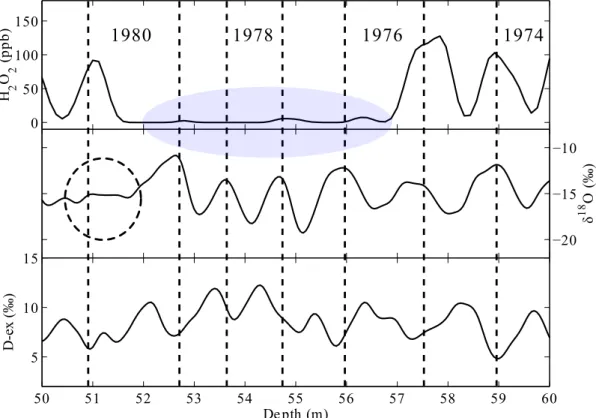
2.4 H2O2,δ18O and D-ex records are shown, from depth 10 – 20 m. The dashed vertical line represents the beginning of each year. The green ellipse indicates the anomalous peak in H2O2 men-tioned in the text. Because the resolution of the H2O2 and isotope measurements was different (see Section 2.2.1), H2O2 were re-sampled to a regular 12 cm grid, and smoothed with a Gaussian filter of width σ = 1 point; δ18_{O and D-ex were} re-sampled to a regular 5 cm grid, and smoothed with a Gaussian of width σ = 2.4 points. . . 41 2.5 An example of the annual year dating process. H2O2,δ18O and

D-ex records are shown, from depth 50 – 60 m. The dashed vertical line represents the beginning of each year. The dashed circle indicates the anomaly in δ18O, and the grey ellipse in-dicates the anomalous region of H2O2. See the text for more details. Due to the resolution of H2O2 and isotope measure-ment being different (see Section 2.2.1), H2O2 were re-sampled to a regular 12 cm grid, and smoothed with a Gaussian filter of widthσ = 1 point; δ18_{O and D-ex were re-sampled to a regular} 5 cm grid, and smoothed with a Gaussian of widthσ= 2.4 points. 42 2.6 Comparison of (a) δ18_{O, (b) D-ex, (c) Na}+_{, (d) MSA, and (e)}

SO2₄− records from MI0910 (black solid line), MIp0910 (green dashed line) and MI0809 (red dotted line). . . 44 2.7 nssSO−₄2 records corresponding to major volcanic events (a)

Pinatubo (1991), (b) El Chichon (1982) and (c) Agung (1963). The dashed vertical line represents the beginning of each year. 46 2.8 Figure showing the dating errors combined in quadrature (solid

line) and linearly (dashed line). Negative error represents an ambiguous seasonal cycle counted as a year marker. Positive error represents an ambiguous seasonal cycle not counted as a year marker. . . 48 2.9 Ninety-seven year record of H2O2(a),δ18O (b),δD (c), and D-ex

(d). All data were re-sampled to a 0.1 year grid and smoothed with a Gaussian filter of width σ=1 point. . . 50 2.10 Average seasonal cycles of a) H2O2, b) δ18O, c) δD, (d) D-ex

for the entire MI0910 record. The error bars show the standard error of the mean. . . 51 2.11 Trace ion chemistry data: a) Na+, b) Cl−, c) MSA, and d) SO2₄−.

(13)

2.12 Average seasonal cycles of a) Na+, b) Cl−, c) MSA, d) SO2₄−, e) nssSO2₄−, f) Mg+_{, g) Ca}+ _{and h) NO}−

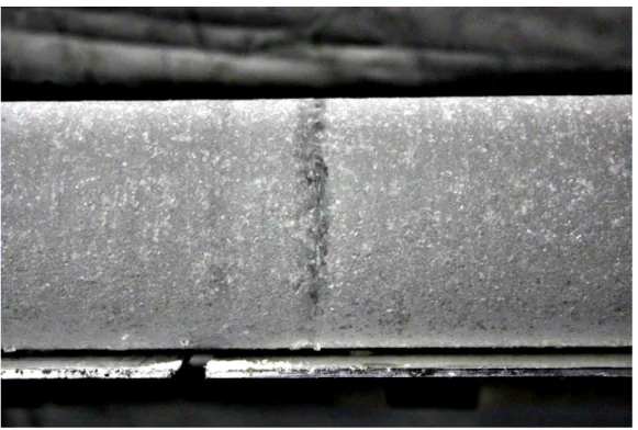
3. The error bars show the standard error of the mean. . . 56 2.13 An example of the crust layers observed in MI0910. . . 59 2.14 Crust layers recorded in MI0910 ice core (blue vertical lines)

with 97 years of H2O2, Na+, and SO24− record. The thickness of the blue lines has been exaggerated, relative to the ice core thickness, in order to enhance visibility. Grey ellipses indicate regions discussed in the text. The firn/ice density is unrelated to the occurrence of crust layers. . . 60 2.15 The number of summer (October – March) crust layers per year

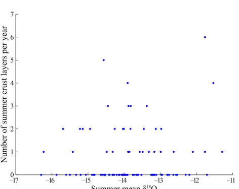
and summer meanδ18O. . . 62 2.16 Figures of a) monthly total crust layers, b) Monthly mean

tem-perature, c) monthly mean number of wind exceed 15 m/s data from six hourly data, d) same as c, but wind speed is less than 5 m/s. . . 63 2.17 Investigating k’: a) linear regression slope, b) correlation

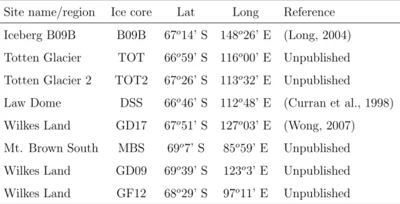
coef-ficient. . . 67 2.18 Comparison of distance from coast and a) sea salt fractionation,

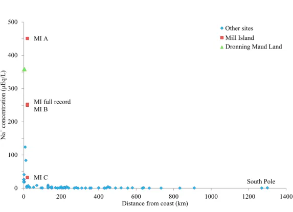
b) mean sodium concentration at several East Antarctica ice core sites. See Table 2.5 for further infomation of other sites. . 69 2.19 Mean Na+ concentrations at Antarctic ice core and snow pit

sites. Na+ concentration isµEq/L and distance is the distance in kilometres from the coast. Figure adapted from Table 1 of Mulvaney and Wolff (1994). Mill Island values are shown as averages during Regime A, B, and C (see the text for details) and averaged for the 97 year Mill Island record. . . 72 2.20 Average seasonal cycle of nssSO2₄−calculated with the corrected

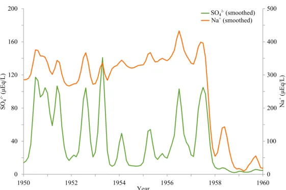
value ofk’. The error bars show the standard error of the mean. Note: volcanic eruption years were excluded from this calcula-tion. . . 73 2.21 Sodium and sulphate records between 1950 and 1960. Data

(14)

LIST OF FIGURES vii

3.1 Time series of a) Na+, b) SO2₄− concentrations, and the ratio of c) δ18_{O, and d) D-ex records over the period from 1913 to} 2009. Each top panel: Data were interpolated to 24 points per year, then smoothed with a Gaussian filter of width σ = 1 point. The x-axis is year, the y axis is month, and color scale is shown in each bottom panel. Each bottom panel: Time series of each species as in Figure 2.9 and Figure 2.11. The background color indicates as color bar of the top panel. Y axis is the concentration/ratio. Regimes A (2009 – 2001), B (2000 – 1934), and C (1933 – 1913) were partitioned using a grey panel. 82 3.2 Average seasonal cycles of a) Na+_{, b) SO}2−

4 , c) δ18O, and d) D-ex for each regime. Regime A: 2001 – 2009 (blue), Regime B: 1934 – 2000 (green), Regime C: 1913 – 1933 (magenta). The x axis shows the month, y axis shows the concentration/ratio. Note that the Na+ concentration is shown with a different scale for regime A (left y axis) and regimes B and C (right y axis). . 86 3.3 Wind rose climatology near Mill Island (grid point: 65.4119◦

S, 100.9375◦ E) from 1979 to 2009. The wind data were de-rived from the NCEP CFSR reanalysis model (Environmental Modeling Center, 2010). . . 88 3.4 The coordinates and names of the five sea ice concentration

data pixels. The red plus symbol indicates the centroid position of the derived time series m, formed by averaging SIC-S and SIC-SIC-SIC-SE. The dark blue rectangle indicates the location of the photograph shown in Figure 3.8. Map courtesy of the Australian Antarctic Division, cOCommonwealth of Australia, 2012. . . 92 3.5 Time series of annual mean SIC-m (red, right y axis), Na+

(orange, left y axis), and SO2₄−(green, left y axis) over the period from 1979 to 2009. Sea ice concentration data were derived from NSIDC (see text). Note that the right y axis is reversed to highlight the high degree of anti-correlation. . . 95 3.6 Time series of annual mean SIC-m (red, right y axis), SIC-W

(blue, right y axis), Na+ _{(orange, left y axis), and SO}2−

4 (green, left y axis) over the period from 1979 to 2009. The horizontal dashed blue line indicates the mean sea ice concentration in SIC-W, dotted blue lines indicate the 1σ standard deviation of the sea ice concentration in SIC-W. Sea ice concentration data were derived from NSIDC (see the text for details). Note that the right y axis is reversed to highlight the high degree of anti-correlation. . . 97 3.7 Schematic diagram of a hypothetical sea-salt transport

(15)

3.8 An aerial photo over Bowman Island on 11th February, 1947. The circle (a) shows an example of the vertical discontinuity from sea level to the ice cap. The circle (b) demonstrates a clear snow ramp. Some scale is provided by cross-referencing with the rectangle in Figure 3.4. Photo courtesy of the Australian Antarctic Division, cOCommonwealth of Australia, 2015. . . 101 3.9 Annual variations in SIC-m, SIC-W, Na+, and SO2₄− over the

period from 1979 to 2009. The x axis is year, y axis is month, and the color shows sea ice/trace ion concentration. Each pixel shows the monthly mean concentration of associated species. Chemical data were interpolated to 12 data points per year. No filtering was used. . . 102 3.10 MODIS images of the Shackleton Ice Shelf and Mill Island area.

Green dashed line divides fast ice and ice shelf. . . 104 3.11 MODIS images of the Shackleton Ice Shelf and Mill Island area. 105 3.12 Concentrations of Na+_{(red solid line), Mg}2+_{(green dashed line)}

and MSA (purple solid line) for (a) 2005 – 2010, (b) 1925 – 1930. No data smoothing was performed. . . 110 3.13 A photo of an Automatic Weather Station covered by thick rime

ice at Roosevelt Island (79◦25’ S, 162◦00’ W), 23rd _October,

2011. Photo provided by N. Bertler. . . 116 4.1 An example of the linear monthly dating process for 2009. The

dashed line shows the δ18_{O ratio time series, and the solid line} shows the monthly meanδ18_{O ratio. The vertical lines partition} a year equally into 12 portions. The uncertainty of the δ18O measurements is <0.1. . . 131 4.2 An example showing the precipitation-weighted monthly dating

method using the CFSR precipitation time series for 2009. The dashed line shows the δ18_{O ratio time series, and the solid line} shows the monthly meanδ18_{O ratio. The vertical lines partition} the year according to the proportion of precipitation in each month. Inset: Monthly precipitation proportion from CFSR output in 2009. . . 133 4.3 An example showing the precipitation-weighted monthly

(16)

LIST OF FIGURES ix

4.4 Mill Island density and strain-corrected annual snow accumu-lation (dashed line) and Gaussian smoothed (σ = 1.5 year) ac-cumulation (solid line). The dash-dotted line shows the line of best fit before and after the break point (1999). The break point was calculated using the Mudelsee (2009) break function regression. . . 136 4.5 Annual snow accumulation and precipitation records from Mill

Island (blue line), CFSR (green line), AMPS (red dashed line), ERA-interim (light blue line) and RACMO (orange line). Mill Island snow accumulation was converted into millimetres of wa-ter equivalent (mmWE). . . 138 4.6 Annual snow accumulation and precipitation records from Mill

Island (blue line), DSS (red line), Casey Station (orange line), Mirny Station (black line), and CFSR at Mill Island (green line). Snow accumulation was converted into millimeters of wa-ter equivalent (mmWE). . . 142 4.7 High- and low-pass filtered annual accumulation records from

Mill Island (blue line) and DSS (red line). Top panel: High-pass filtered accumulation, using a cut-off frequency of fc = 3 years; Bottom panel: Low-pass (Gaussian) filtered accumulation (σ= 1.5 years). . . 143 4.8 The high- and low-pass filtered annual accumulation records

from Mill Island (blue line) and Mirny Station (green line). Top panel: High-pass filtered accumulation, cut-off frequency

fc = 3 years; Bottom panel: Low-pass (Gaussian) filtered accu-mulation (σ= 1.5 years). . . 145 4.9 Katabatic wind streamlines overlaid with the locations of Mirny

Station (green diamond), Mill Island (blue star), and Law Dome (red circle). The figure was obtained and modified from Figure 3, Parish and Bromwich (1987). . . 147 4.10 The composite map of precipitation co-variability modified from

Figure 1, Monaghan et al. (2006), overlaid with the locations of Mirny Station (green diamond), Mill Island (blue star), and Law Dome (yellow circle number 7). Detailed information for this figure is given in Monaghan et al. (2006). . . 148 4.11 The phase of ZW3 at the 500-hPa geopotential height field with

(17)

4.12 Annual mean Mill Island δ18O (blue), DSS δ18O (red), Casey Station temperature (yellow), Mirny Station temperature (black), CFSR temperature at Mill Island (green), GF08 (AWS) tem-perature (magenta). . . 152 4.13 Left panel: The monthly mean temperature from CFSR (a,

orange dashed line) and monthly meanδ18_{O record derived from} the linear precipitation assumption (b, blue solid line), from the precipitation time series-weighted dating method (c, black line), and the precipitation climatology-weighted dating method (d, green line). . . 155 4.14 Left panel: The monthly mean temperature anomaly from CFSR

at Mill Island (a, orange dashed line) and the monthly mean

δ18O anomaly record derived from the linear precipitation as-sumption (b, blue solid line), from the precipitation time series-weighted dating method (c, black line), and the precipitation climatology-weighted dating method (d, green line). Right panel: climatologies of the CFSR temperature at Mill Island (orange dashed line) and monthly mean δ18_{O calculated with the} lin-ear precipitation assumption (blue line), the precipitation time series-weighted dating method (black line), and the precipita-tion climatology-weighted dating method (green line). The er-ror bars show the standard erer-ror of the mean. . . 158 4.15 Climatology of the precipitation proportion for the period of

a) 1979 – 1989 (blue), b) 1990 – 1999 (green), c) 2000 – 2009 (magenta), and d) 1979 – 2009 (black). The error bars show the standard error of the mean. The horizontal dotted line shows the linear monthly precipitation proportion (∼0.0833). . . . 160 4.16 Annual mean δ18_{O (blue) and annual mean} _δ18_{O corrected}

us-ing the precipitation-weighted monthly datus-ing method (black), from 1979 – 2009. . . 162 4.17 An example showing the summer and winter windows: Top

panel, Black solid line shows δ18O record. X axis is ice core depth, y axis is δ18_{O ratio (}_{). The vertical red dashed lines} show the beginning of each year, i.e., the mid-summer markers, and the vertical blue dotted lines show mid-winter markers; bottom panel, associated depth of sodium (orange, left y axis) and MSA (purple, right y axis) records. . . 165 4.18 A scatter plot of CFSR mean temperature for December to

(18)

LIST OF FIGURES xi

4.19 a) Mill Island borehole temperature (green solid, Roberts et al., 2013), b) CFSR temperature at Mill Island (November to April [magenta dashed line], May to October [cyan dashed line], Novem-ber to OctoNovem-ber [black dashed line], and January to DecemNovem-ber [orange dashed line]), and c) Mill Island δ18_{O ratio (summer} 10 % window mean [red], winter 10 % window mean [blue], mean of summer 10 % and winter 10 % windows [black], and annual mean [orange]). . . 173 A.1 The ambiguous part of the H2O2, δ18O and D-ex records from

depth 10 – 20 m. The dashed vertical line represents the begin-ning of each year. . . 187 A.2 The ambiguous part of the H2O2, δ18O and D-ex records from

depth 50 – 60 m. The dashed vertical line represents the begin-ning of each year. . . 188 A.3 The ambiguous part of the H2O2, δ18O and D-ex records from

depth 80 to 90 m. The dashed vertical line represents the be-ginning of each year. . . 190 A.4 The ambiguous part of the H2O2, δ18O and D-ex records from

(19)

1.1 The location, depth, and drill date of ice cores recovered from Mill Island. . . 8

2.1 Mill Island ice core information . . . 31 2.2 Mean concentration, standard deviation, sample number, and

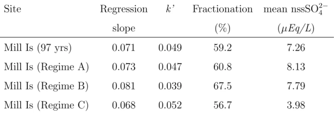
standard error of the mean of the trace ion species from the complete 120 m MI0910 ice core. . . 37 2.3 Volcanic eruption records as identified from nssSO2₄− peaks in

the Mill Island and LD ice cores during 1913 – 2009 (Palmer et al., 2001; Plummer et al., 2012). Years are reported as deci-mal fractions of a year. . . 46 2.4 The correctedk value and mean nssSO2₄− concentration in each

regime. . . 68 2.5 Site information of the other ice core sites in Figure 2.18. Data

were derived from Wong (2007); Long (2004) and M. Curran (Personal communication, 2014). . . 71

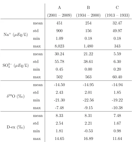
3.1 Mean concentrations, standard deviation, minimum and maxi-mum values of the Na+_{, SO}2−

4 ,δ18O, and D-ex in each regime. 84 3.2 Correlations between CFSR wind speed at Mill Island and

con-centration of Na+ _{and SO}2−

4 during winter and summer and for the annual average. Bold values indicate p<0.05. . . 90 3.3 Correlation coefficients between annual mean sea ice

concentra-tion at each pixel and the annual mean concentraconcentra-tion of Na+ and SO2₄−. Bold numbers indicate p<0.01. . . 93

(20)

LIST OF TABLES xiii

3.4 Correlation coefficients between annual mean sea ice concentra-tion at SIC-m and the annual mean concentraconcentra-tions of Na+ _and SO2₄− during the periods of 1979 – 2009 (SIC-mAB), regime A

(2001 – 2009, SIC-mA), and regime B (1979 – 2000, SIC-mB).

Bold numbers indicate p<0.03. . . 94 4.1 The atmospheric model datasets assessed in this chapter. Note

that ERA-interim data were obtained only from 1983 to 2009 for trial analyses. . . 128 4.2 The correlation coefficient between Mill Island snow

accumula-tion and each atmospheric model dataset assessed in this chap-ter, the range of r with 95 % confidence, and the percentage of mean precipitation compared to the Mill Island mean precipi-tation. The p value and number of degrees of freedom used is also shown in here. The AMPS time series is too short for a meaningful significant test. . . 139 4.3 The correlation coefficient (r) and significance (p value) between

each pair of annual mean δ18_{O and annual mean temperature} records. Bold font indicates a significant correlation (p<0.05). 153 4.4 CFSR mean periods for summer and winter windows. The left

column shows the starting month. . . 167 4.5 The correlation coefficient between “summer” percentage

win-dow mean δ18O (columns) and “summer” CFSR temperature (rows) for each monthly combination. Red coloured cells indi-cate p<0.05, dark red coloured cells indicate p≤0.01. . . . 168 4.6 The correlation coefficient between winter percentage window

(21)

Introduction

1.1 Basis of the study

Climate change is one of the most important and urgent issues facing hu-mankind. Despite recent intensive, globally-coordinated research efforts, key aspects of the climate system are still poorly understood (IPCC, 2014). Antarc-tica and the Southern Ocean play a criAntarc-tical role in the global climate sys-tem. Understanding past climate variability is crucial for interpreting the present climate and understanding the future state of the global climate sys-tem. Highly valuable historical records of several key climate parameters are contained within chemical records of Antarctic ice cores, e.g., sea ice extent (e.g., Curran et al., 2003; Abram et al., 2013), the dominant modes of large-scale atmospheric variability in the high-latitude Southern Hemisphere (e.g., Goodwin et al., 2004; Steig et al., 2013), and past temperature (e.g., van Om-men and Morgan, 1997; Schneider et al., 2006). One aim of this thesis is to

(22)

1.2. SIGNIFICANCE AND AIMS 2

extend studies such as these using high resolution records from Mill Island, a new ice core site in East Antarctica. The Mill Island site was selected based on an expected high accumulation rate, and was expected to provide a straight-forward high resolution climate record.

1.2 Significance and aims

Mill Island (65◦ 30’ S, 100◦ 40’ E) is situated in East Antarctica, at a location experiencing high and consistent precipitation, making it an ideal location for producing high-resolution and high-quality proxy climate records. A thor-ough glaciochemical investigation of the Mill Island ice core will contribute to answering the key questions, “What changes are occurring in the climate of Antarctica and the Southern Ocean?” and “What are the links between these changes and the global climate system?” Records of these climate proxies will contribute to improving models of the climate system and projections of the future state of the climate.

(23)

knowledge gap, and this project contributes to that plan (PAGES 2k Consor-tium et al., 2013).

The aims of this thesis are:

1. To produce high resolution, well-dated records of water stable isotopes (δ18_O, _δ_{D), and trace ion chemistry (sea salts, sulphate,} methanesul-phonic acid) at Mill Island;

2. To investigate the seasonal and interannual variability of sea salts, in order to understand climate factors influencing Mill Island; and

3. To perform a regional comparison of δ18_{O and snow accumulation rate} with nearby existing climate records from ice cores, observational sta-tions, and atmospheric models, in order to determine the optimal method for temperature reconstruction at Mill Island.

This thesis will show that the Mill Island ice core records are unex-pectedly complex, with strong modulation of the trace chemistry on long timescales. While this makes interpretation of the record challenging, this thesis will examine potential reasons for the complexity and provide evidence for significant regional influence as a result of long term variability of regional sea ice cover.

(24)

1.3. SITE INFORMATION 4

collected from Mill Island are presented here. The following literature review focuses on snow accumulation, water stable isotopes and trace ion chemistry, particularly sea salts, non sea salt sulphate (nssSO2₄−), and methanesulphonic acid (MSA). The review provides background information and discussion of relevant issues that are important in the chapters that follow.

1.3 Site information

Mill Island (65◦ 30’ S, 100◦ 40’ E) is a small island (∼45Ö35 km), rising ∼500 m above sea level, located in East Antarctica. It is connected to the Antarctic continent by the Shackleton Ice Shelf. The relatively low elevation and close distance to the ocean suggests the potential for significant input of maritime air to the snow falling at Mill Island. Mill Island is located ap-proximately 500 km east of Law Dome, 350 km west of Mirny Station, 60 km north of the exposed rock formation known as Bunger Hills, and lies at the northern edge of the Shackleton Ice Shelf in Queen Mary Land (Figure 1.1). The Shackleton Ice Shelf has experienced large changes in the past (Young and Gibson, submitted, 2013) which are likely periodic in nature, and not necessarily forced by changes in the local climate.

(25)

(26)

1.3. SITE INFORMATION 6

northerly climate record for East Antarctica (Roberts et al., 2013). Mill Island experiences a polar maritime climate and high precipitation, particularly on its eastern flank, due to moist and warm air masses from the Southern Ocean brought onshore by low pressure systems. The site also experiences dry and cold air associated with strong katabatic winds from the continent and low level cloud, fog and rime formation over the summit caused by localised summer sea-breezes associated with nearby sea-ice breakout (Roberts et al., 2013). Records from Mirny Station show that the monthly mean temperature is below zero throughout the year (Turner and Pendlebury, 2004), suggesting that Mill Island has only a small chance of experiencing melt, particularly at the∼500 m elevation summit. The high precipitation rate and minimal melt makes Mill Island an ideal site from which to extract high resolution climate records for the Southern Hemisphere.

1.3.1 Drilling campaign

(27)

1236). The team spent three weeks in the field, and drilled one 120 m main ice core (MI0910) and seven shallow (from∼5 m to 10 m) firn ice cores. However, due to harsh weather conditions, other observational data such as snow pit and ground penetrating radar (GPR) data were not acquired. Table 1.1 gives information on each of the ice cores. Figure 1.2 shows the location of each ice core site. Two shallow cores, MIp0910 and MI0kp0910, were derived from the same site as the main core, MI0910. Other shallow cores were taken at a 5 km distance from MI0910 in directions of north, north-east, east, south, and west (MIN5kp0910, MINE5kp0910, MIE5kp0910, MIS5kp0190, MIW5kp0910, respectively).

This thesis focuses on the main (MI0910) ice core record, with the sup-port of two shallow ice cores MIp0910 and MIp0809. The Eclipse ice core drill, an electromechanical dry ice-coring drill detailed in (Blake et al., 1998), used for the main core required ∼2 m of trench for operation. Thus, the main core does not have samples from the surface to the base of the trench. This section of the record was obtained from shallow ice cores drilled with a different drill. The MI0910 record is supplemented at the top by the MIp0910 record.

1.3.2 Previous studies using the Mill Island shallow ice

cores

(28)

(29)

!

! !

! MI0910

MIE5kp0910 MI0809

MIN5kp0910

MIW5kp0910

MIS5kp0910

MINE5kp0910 N

Mill Island

Shackleton Ice Shelf

Southern Ocean

(30)

1.4. BACKGROUND ON ICE CORE PROXIES 10

Sodium (Na+) originates from open water sea salts and frost flowers on the surface of sea ice. Seasonal variations in Na+ _{concentrations were linked to} synoptic storm variability, and the partitioning between Na+ _{sources within} each season was determined by sea ice extent and the dominant synoptic con-ditions. A higher contribution from frost flowers was evident in seasons where increased sea ice was coupled with synoptic conditions that promote their for-mation and transportation. Snow accumulation at MIp0910 was found to be ∼42% higher than at MIp0809 in the winter of 2008, due to the location of MIp0809 location on the leeward slope of Mill Island. Summer accumulation variability was found to be linked to the blocking of circumpolar westerlies, with enhanced northerly flow generating a higher snow accumulation rate at Mill Island. Domensino (2010) concluded that there was no significant snow accumulation variability within the spatial array of shallow core sites (repre-senting a spatial separation of∼15 km). Snow accumulation differences across the island are the result of topographic variations, not spatial variability of precipitation.

1.4 Background on ice core proxies

(31)

climate proxies.

1.4.1 Snow accumulation

Melting of the Antarctic Ice Sheet plays an important role in sea level rise, however, it is difficult to assess the current contribution of the Antarctic Ice Sheet to sea level rise due to uncertainties in net surface mass balance (SMB) over most of the continent. SMB data are often of limited spatial and temporal representativeness, and current knowledge of SMB is confounded by measure-ment inaccuracy, and lack of quality control (Magand et al., 2007).

(32)

(e.g., Lenaerts et al., 2013).

The snow accumulation record is also a proxy for circumpolar atmo-spheric circulation (Goodwin et al., 2003), and for synoptic scale storm events, not only at the ice core site but also in the wider area (Cohen and Dean, 2013). A link between snow accumulation at Law Dome (LD) and precipitation in south-west Western Australia was also identified (van Ommen and Morgan, 2010).

1.4.2 Water stable isotopes

(33)

Mechanism of water isotopic fractionation, and the role of δ18O,δD, D-ex, and δ17_O

The proportions of water stable isotopes, H216O, H217O, H218O and HD16O, are generally uniform throughout the ocean (Dansgaard, 1964; Angert et al., 2004). When water evaporates from the surface of the ocean, heavier iso-topes (i.e., H217O, H218O and HD16O), tend to preferentially remain in the ocean. Thus, the water vapour above the surface of the ocean is enriched in H216O and other light isotopic variants. As the water vapour is transported to higher latitudes, the airmass cools down, and molecules with heavier isotope preferentially precipitate to avoid supersaturation. Thus, the water vapour becomes more depleted in heavier isotopes molecules as the surrounding air temperature cools (Morgan, 1982). The ratio of heavier isotopes (δ) relative to Standard Mean Ocean Water (SMOW), is calculated with the following equation (Dansgaard, 1964; Paterson, 1994)

δ= αsample−αSM OW

αSM OW

×103 (1.1)

whereαis the concentration of the isotopes in sample (αsample), and in SMOW

(αSM OW). The final δ values in precipitation at the site depend mainly on

(34)

as proxies for site temperature.

While δ18O andδD both give past temperature information, the combi-nation of these two isotopes and deuterium excess (D-ex), provides additional information on past temperature and evaporative conditions over the ocean (Bradley, 1999; Delmotte et al., 2000). D-ex reflects the different behaviours of HD16_{O and H}

218O occurring during the processes of evaporation and conden-sation (Delmotte et al., 2000), and thus has been used for deriving moisture source information. However D-ex is influenced by the relative humidity of the oceanic source region as well as sea surface and site temperatures, making it difficult to use as a sole indicator for moisture source conditions (Landais et al., 2008). D-ex is calculated with the equation

D-ex=δD− 8δ18O

(Paterson, 1994; Delmotte et al., 2000).

Until recently, the depletion of H217O in precipitation was assumed to carry no additional information to that of H216O and H218O (Angert et al., 2004). Furthermore, measurement of δ17_{O was impractical until recently} (Landais et al., 2008). Angert et al. (2004) suggested the potential use of

(35)

δ18O as a temperature proxy

Since δ18_{O and} _δ_{D values in precipitation depend on the temperature at the} moisture source (i.e., the sea surface temperature, SST) and at the precipita-tion site, and because the SST is more stable than the air temperatures at high latitudes, the dependence on SST is relatively smaller, so values of δ18_{O and}

δD in polar snow both strongly reflect the temperature at the site and time of precipitation. Thus, measuring these ratios as a function of depth in an ice core can be interpreted as a record of site temperature (Paterson, 1994). δ18_O and temperature generally display a linear relationship, given by the following empirical equation

δ18O =αT +β (1.2)

(36)

1.4.3 Trace ion chemistry

The atmosphere contains various soluble and insoluble impurities originat-ing from three sources: The ocean (e.g., sea salt); the surface of the con-tinents (e.g., terrestrial dust); and biogenic or anthropogenic gas emissions (e.g., dimethyl sulphide [DMS] and hydrogen chloride [HCl]) (Legrand and Mayewski, 1997). Primary aerosols, e.g., sea salt and dust, are directly in-troduced into the atmosphere by wind from marine and continental surfaces. Secondary aerosols are produced within the atmosphere during oxidation of trace gases (Legrand and Mayewski, 1997). Trace ion records represent a wide range of environmental information. For example, Plummer et al. (2012) in-vestigated nssSO2₄− from the Law Dome ice core to determine the timing of volcanic eruption events over the past 2000 years. Also, Goodwin et al. (2004) and Vance et al. (2013) used sea salt (sodium [Na+]) to investigate large-scale climate phenomena such as the Southern Annular Mode (SAM) and El Ni˜no, respectively. Moreover, sea salt and methanesulphonic acid (MSA) have been studied as proxies for sea ice (Curran et al., 2003; Wolff et al., 2003; Abram et al., 2013). The trace ions measured in this thesis can broadly be categorised into two groups: Sea salt species (Na+_{, Cl}−_{, Mg}2+_{, Ca}2+ _{and a part of SO}2−

(37)

Sea salt: Open ocean and frost flower

Sea salt concentration in Antarctic ice cores is characterised by a winter max-imum and a summer minmax-imum, despite the closer distance to the open ocean during summer (Legrand and Mayewski, 1997). This apparent contradiction leads to a discussion of the source of sea salt. Sea spray (i.e., bursting of air bubbles during wave breaking) from the open ocean is the main source of sea salt, and the increased storm activity during winter causes the winter time maximum (Wagenbach et al., 1998a; Benassai et al., 2005). Snow pit studies have also shown high sea salt concentrations in snow following the passage of marine air advected to higher latitudes via cyclonic systems (McMorrow et al., 2001). During winter, the ratio of chloride (Cl−) to Na+ in ice cores is close to that of bulk seawater, suggesting that both Na+ _{and Cl}− _{originate from sea} salt. This ratio changes in summer due to additional Cl− input from (HCl), especially farther inland (Legrand and Mayewski, 1997). Therefore, Na+ is generally used as a representative of sea salt, and it has also been considered as a proxy of wind speed and storminess (Legrand and Mayewski, 1997; Curran et al., 1998; Wagenbach et al., 1998a).

(38)

Na+ (Rankin et al., 2002). There are four steps for frost flower formation. Firstly, the brine in thin young sea ice is transported toward the relatively colder surface due to the thermomolecular pressure gradient (Martin et al., 1996). The brine accumulates as both a liquid and a slushy layer on the surface of newly formed sea ice. Secondly, the surface brine evaporates into the colder atmospheric boundary layer which creates a thin (1 – 3 cm thickness) layer of water vapour just above the surface. This water vapour layer is supersaturated with respect to ice, and promotes deposition of crystal growth i.e., frost flowers (Rankin et al., 2002). Next, beneath the frost flowers, a saturated brine slush layer forms (2 – 4 mm thickness). Finally, surface tension effects cause the incorporation of the surface brine onto the frost flowers, resulting in high salinity on the frost flowers (Hall and Wolff, 1998; Rankin et al., 2002). These fragile frost flowers are expected to efficiently aerosolise (Rankin et al., 2002). Frost flowers have a salinity of almost three times the concentration of sea water attributing to the high salt concentration in the ice core during winter (Rankin et al., 2000). Thus, the sea-ice zone around Antarctica (particularly coastal regions) is an important source of sea salt aerosols (Abram et al., 2013).

(39)

around Antarctica may be an important source of sea salt aerosols, especially in coastal Antarctica, and thus the sea salt record may be useful as a sea ice proxy (Wolff et al., 2003; Abram et al., 2013).

Non sea salt sulphate

Sulphate in ice cores originates from several sources. They include sea salt as a primary source, continental dust, large volcanic eruptions, and biological activity (Legrand and Mayewski, 1997; Curran et al., 1998). nssSO2₄− is pro-duced by the oxidation of sulphur dioxide (SO2), which is derived from the oxidation of reduced organic sulphur gases, emitted mainly from the ocean and volcanoes. Thus, nssSO2₄− is believed to indicate marine biogenic activity as well as being a volcanic activity indicator (Curran et al., 1998). nssSO2₄− is calculated by subtracting sea salt sulphate from total sulphate.

[nssSO2₄−] = [totalSO2₄−]−k∗[X] (1.3)

(40)

core nssSO2₄− concentration records during winter (Wagenbach et al., 1998a; Curran et al., 1998). These deficiencies are generally well correlated with sea salt (Na+_{or/and Cl}−_{) concentration (Wagenbach et al., 1998a), and generally} occur when the wind blows from a new sea-ice formation area (Hall and Wolff, 1998). These SO2₄− depleted aerosols originate from frost flowers.

Methansulphonic acid (MSA)

MSA has only one source: Oxidation of DMS. DMS is a volatile sulphur gas produced by oceanic phytoplankton (Legrand and Mayewski, 1997; O’Dowd and de Leeuw, 2007). Those phytoplankton are particularly abundant in the sea ice zone, and produce DMS during summer months (Curran et al., 2002). Therefore, MSA is deposited in summer, and is used as a proxy for marine biogenic activity as well as sea ice extent (Welch et al., 1993; Legrand and Mayewski, 1997; Curran et al., 2003; Abram et al., 2013). Although the mech-anism of MSA production within the sea ice zone is not yet fully understood, MSA is the most robust sea ice proxy at high accumulation coastal ice core sites (Abram et al., 2013).

(41)

of phase with nssSO2₄− and finally peak in winter ice (Mulvaney et al., 1992; Wolff, 1996). This winter MSA peak is thought to migrate from summer snow, since MSA deposition in winter is highly unlikely (because MSA depends on production of marine biological activity, and nssSO2₄−peaks remain in summer layers). Possible MSA migration occurs when MSA diffuses in either a vapor or liquid phase, and becomes locked in a winter layer by forming an insoluble salt with a cation (Pasteur and Mulvaney, 2000). Therefore, special atten-tion is required to interpret the MSA record. However, because migraatten-tion is likely contained within a single annual layer, such migration should not affect multi-year average MSA values (Curran et al., 2002).

1.5 Thesis structure

(42)

1.5. THESIS STRUCTURE 22

(43)

Dating and glaciochemistry of the high

resolution Mill Island ice core

2.1 Introduction

This chapter presents high resolution, well-dated records of water stable iso-topes and trace ion chemistry from the main Mill Island 120 m ice core (MI0910) which will be used as climate proxies in the following chapters. The visual stratigraphy of MI0910 is documented in order to investigate the influence of coarse-grained layers on the measurement results. Sea salt fractionation is also investigated, in order to calculate non sea salt sulphate (nssSO2₄−).

Accurate ice core dating is crucial for calibration and interpretation of ice core records. Many different dating methods have been used in the past including counting seasonal variations, radioisotopic methods, and reference horizons (Legrand and Mayewski, 1997; Bradley, 1999). In cores with sufficient accumulation rate, many trace records show distinct seasonal varieties which can be used to identify annual layers. For example, hydrogen peroxide (H2O2) shows clear seasonal variability in Antarctic snow due to its dependence on

(44)

2.1. INTRODUCTION 24

tropospheric photochemistry formation processes (Logan et al., 1981; Sigg and Neftel, 1988; van Ommen and Morgan, 1996). Water isotope ratios (e.g., δ18_O) also show seasonal cycles with more highly fractionated values in winter snow than in summer snow due to the close relationship with atmospheric temper-ature, as discussed in Chapter 1 (Bradley, 1999). Major trace ion chemicals (e.g., sodium [Na+_{], chloride [Cl}−_{], nitrate [NO}−

3], calcium [Ca2+]) also gen-erally show pronounced seasonal variations and can be used for annual layer counting (Curran et al., 1998; Bradley, 1999). Various dating methods are used depending on the required accuracy and snow accumulation rate (Legrand and Mayewski, 1997). Using several records for dating is an effective method for counting annual layers, because different mechanisms express the seasonal cy-cle in different parameters. Multi-record layer counting can minimise dating uncertainties (e.g., Dansgaard et al., 1982; Morgan et al., 1997).

(45)

(Langway, 1970). Such layers can form from a small amount of liquid wa-ter condensing onto a surface or near-surface crust (Das and Alley, 2005). Hence the presence of fog may cause such a layer. Strong seasonal and diurnal temperature gradients drive grain-size growth (Linow et al., 2012). Strong continuous wind during precipitation hiatuses can remove surface snow. As a consequence, larger grains of near-surface snow are exposed, absorbing more solar radiation and accelerating grain growth and metamorphosis of the near-surface snow (Goodwin, 1990; Das et al., 2013). These grain metamorphism processes can occur rapidly (Langway, 1970; Alley, 1988). The cause of each layer is difficult to explicitly investigate by close inspection alone (Kinnard et al., 2008). Thus all such layers observed in MI0910 are here termed “crust layers” for convenience.

(46)

2.1. INTRODUCTION 26

and Wolff, 1998; Wagenbach et al., 1998a). Fractionation of sea salt happens when a constituent of sea water is removed, leaving behind a deficit of that species (Hall and Wolff, 1998). Sea salt fractionation is the depletion of sea salt sulphate relative to sodium in snow and ice cores and has been identified at many coastal Antarctic sites during winter period (Minikin et al., 1998; Rankin et al., 2002). These depleted aerosols most likely originate from frost flowers which form on the surface of new sea-ice when the surface temperature is below

=8, and the surface wind speed is low (Perovich and Richter-Menge, 1994; Rankin et al., 2000). Mirabilite (Na2SO4·10H2O) crystallises below =8in brine which accumulates at the top of the sea ice surface. Hence the remaining brine becomes depleted in SO2₄−(Wagenbach et al., 1998a). As a consequence, frost flowers which form in surface temperatures below =8 are depleted in SO2₄− (Rankin et al., 2000). Details of frost flower formation are described in Section 1.4.3.

(47)

2.2 Method

2.2.1 Ice core analysis

The Mill Island ice cores were processed and analysed in the glaciology labo-ratory at ACE CRC, Hobart, Australia. This section describes the analytical methods used, including the ice core processing, and measurements for hydro-gen peroxide, water stable isotopes, and trace ion chemistry analysis.

Ice core processing

(48)

2.2. METHOD 28

melted in a refrigerator overnight to avoid MSA loss (Abram et al., 2008), then refrozen again. The refrozen samples were melted prior to analysis. All tools used for processing ice cores were carefully pre-cleaned with deionised ultra-clean Milli-Q water (resistivity > 18 MΩ–cm), and polyethylene gloves were worn during the ice core processing, to minimise contamination.

Hydrogen peroxide (H2O2) measurement

Hydrogen peroxide (H2O2) is influenced by photochemical processes. This provides a strong seasonal variation, with a peak during summer when short-wave radiation fluxes are higher. Thus, it is useful for dating ice cores (Sigg and Neftel, 1988). Hydrogen peroxide measurements were carried out at ACE CRC, using a fluorescence detector as detailed by van Ommen and Morgan (1996). A 4 cm sample was analysed every 8 cm from the surface to a depth of 25 m, then every 12 cm for the rest of the core due to time constraints.

Water stable isotope measurement

(49)

auto-sampler (LAS EuroAS300). Analytical precision for δD is <0.5 and for δ18_{O is} _< _0.1 _{, and values are expressed relative to the Vienna} Stan-dard Mean Ocean Water 2 (VSMOW2). D-ex was then calculated from the measured δD andδ18O using the following equation

D-ex =δD−8×δ18O (2.1)

(Paterson, 1994).

Trace ion chemistry measurement

Trace ion chemical measurements were carried out using a suppressed ion chromatograph (IC) as detailed by Curran and Palmer (2001). Samples were melted overnight in a refrigerator prior to analysis. Due to the high sea salt concentration, the melted samples were diluted 50 times in autosampler polyvials using a micropipette within a laminar flow. Further dilutions (5 to 100 times) were completed according to the sea salt concentration from the result of the initial analysis.

(50)

2.2. METHOD 30

study were CH3SO₃− (MSA), Cl−, NO−₃, SO₄2−, Na+, K+, Mg2+, and Ca2+. The nssSO2₄− record was then calculated using the formula

[nssSO2₄−] = [SO2₄−]−kN a×[Na+] (2.2)

wherekN a is sea salt ratio of SO24−to Na+, 0.120 (Mulvaney and Wolff, 1994). All trace ions were calibrated using diluted standards (Curran and Palmer, 2001) expressed in concentrations of microequivalents per litre (µEq/L).

2.2.2 Dating

(51)

Ice core Lat Lon Depth (m) Drill date MI0910 65o _{33’ 10” S} ₁₀₀o _{47’ 06” E} ₁₂₀ _2010-01-18

MIp0910 65o _{33’ 10” S} ₁₀₀o _{47’ 06” E} _10.57 _2010-01-15

MIp0809 65o _{33’ 25” S} ₁₀₀o _{33’ 26” E} _16.69 _2009-01-22

Table 2.1: Mill Island ice core information

2.2.3 Stratigraphy

Visual stratigraphy observation was achieved by counting and logging the crust layers. The crust layers were measured for thickness and counted manually during processing of the ice core. An example of the crust layers is given in Figure 2.13, and the results are presented in Figure 2.14.

2.3 Results and discussion

2.3.1 Measurement results

This section presents the full records of hydrogen peroxide (H2O2), water stable isotope (δ18_O,_δ_{D), and trace ion chemistry. The top part of all records (depth} 0 m to ∼2 m) was supplemented by the MIp0910 record.

H2O2 and water stable isotope records

(52)

2.3. RESULTS AND DISCUSSION 32

at depth∼50 to 60 m and 80 to 90 m where there is an observed loss of H2O2 (Figure 2.1 a). Such a loss of H2O2 seasonality has previously been attributed to transient melt events (van Ommen and Morgan, 1996). However this is not necessarily the case at Mill Island. Further discussion of this loss of H2O2 is presented in Section 2.3.4. Because of the unambiguous peak distribution outside of these two regions (i.e., depth ∼50 to 60 m and 80 to 90 m), the H2O2 record was primarily used for dating MI0910 (Section 2.3.2). The H2O2 record shows a baseline drift below∼100 m which is attributed to calibration problems. Despite this, the data show strong seasonal variations which are sufficient to assist annual layer counting throughout most of the record.

The water stable isotope (δ18_O, _δ_{D) and the deuterium excess (D-ex)} records also show annual cycles throughout the core (Figures 2.1 b, c, and d respectively). Oxygen isotope (δ18O) and deuterium (δD) show similar fea-tures.

Trace chemistry record

(53)

0 5 0 1 0 0 1 5 0 2 0 0 − 2 0 − 1 5 − 1 0 − 1 6 0 − 1 4 0 − 1 2 0 − 1 0 0 − 8 0 − 6 0 0 2 0 4 0 6 0 8 0 1 0 0 1 2 0 5 1 0 1 5 H 2 O 2

(ppb) D (‰) δ

δ 18

O (‰) D-ex (‰)

Depth (m)

(a) (b) (c) (d)

(54)

(Legrand and Mayewski, 1997). However the results for the trace ion chemistry at Mill Island show clear seasonality only in the top ∼20 m of the ice core. The seasonality in trace chemistry either disappears, or shows incoherent peaks below∼20 m (Figure 2.2). The baselines of Na+ and Cl−are also higher from ∼20 to ∼100 m depth.

The mean concentration and standard deviation of each trace ion species is presented in Table 2.2. The standard deviation is higher than the mean concentration for all species. The mean concentration of all trace ion species (except nitrate) is higher at Mill Island than at LD (Curran et al., 1998). Further details and a comparison with other sites is provided in Figure 2.18 and Chapter 3.

The next section presents the dating of MI0910 using these records. Further discussion and interpretation of all records is given after the dating section.

2.3.2 Dating

Mill Island main ice core (MI0910)

(55)

0 5 0 0 Na + (µE q/L ) 0 5 0 0 Cl − (µE q/L ) 0 0 .5 1 1 .5 2 MS A,(µ Eq /L) 0 2 0 4 0 6 0 8 0 1 0 0 1 2 0 0 5 0 1 0 0 1 5 0 2 0 0 SO 4 2 − (µE q/L ) De p th ,(m ) 1,500 1,000 1,500 1,000

(a) (b) (c) (d)

(56)

0 50

1 0 0 nssSO 4 2−_(µEq/L) 0 1 0 0 2 0 0 3 0 0

Mg2+(µEq/L)

0 20 40 60 Ca2+(µEq/L)

0 2 0 4 0 6 0 8 0 1 0 0 1 2

0 0 0

(57)

(58)

to determine annual layers at this site. H2O2 and δ18O were primarily used to identify annual layers. Where there were ambiguities with these records, D-ex was also used. The trace chemistry record was not used to identify annual layers because seasonal variations are only present in the top ∼20 m of the record (see Section 2.3.1).

The oxygen isotope ratio (δ18_{O) peak was used as a marker of the} be-ginning of the year. This is associated with temperature at the core site (Dansgaard, 1964; Paterson, 1994) and thus presents a maximum value during summer (e.g., at LD, van Ommen and Morgan (1997)). The Mill Island δ18_O record often shows multiple peaks throughout the year which makes it diffi-cult to determine the maximum summer peak in some years. Therefore, the D-ex trough was used to guide the choice of the beginning of the year when required. D-ex commonly shows a summer trough. This feature is thought to be a consequence of open water nearby the site acting as a source of moisture (Delmotte et al., 2000).

Peak picking for the beginning of each year

Figure 2.3 shows an example of choosing a peak as a beginning of a year. Years 2001 and 1998 are relatively simple: There is one clear H2O2 and δ18O peak, with a D-ex trough. Note that the year used in this thesis is A.D.

(59)

0 50 100 150

H 2 O 2

(p

p

b

)

−20 −15 −10

δ

1

8 O

(‰)

20 20.5 21 21.5 22 22.5 23 23.5 24 24.5 25

5 10 15

De pth (m)

2001 2000 1999 1998

a b c d

D-ex (‰)

Figure 2.3: H2O2, δ18O and D-ex records are shown, from depth 20 – 25 m. The black dashed vertical line represents the beginning of each year. The blue dotted lines, a, b, c, and d, demonstrate potential choices for the beginning of 1999. See the text for more details. Because the resolution of the H2O2 and isotope measurements is different (see Section 2.2.1), H2O2 data were re-sampled to a regular 12 cm grid, and smoothed with a Gaussian filter of width

(60)

22.25 m depth. Howeverδ18O shows no peak and the D-ex shows no trough at this depth. The nearest peaks ofδ18_{O, at depths of 21.9 m and 22.6 m (dotted} blue line, a), are potential year markers. The peak at 21.9 m was chosen because of the D-ex trough at the same depth. The lack of a coincident H2O2 peak may arise from loss processes in warm, wet summer snow and/or reduced photochemical production.

The choice of the start of year 1999 was complicated. The clear H2O2 peak indicates an annual layer around 23.25 m depth. However δ18O shows double peaks (dotted blue lines a and d). The D-ex trough does not match with theδ18O peaks. Sinceδ18O does not show a clear trough between the two peaks (dotted lines a and d), the potential year marker could be within the depth range of line a (∼22.6 m) to line d (∼23.5 m). Line c was eventually chosen as the 1999 year marker due to the concurrent H2O2 peak. Since the chemical signals are very complicated at Mill Island, there is no other record available to determine which peak should be picked as the year marker. These differences (dotted lines a to d) do not affect the total number of years which the MI0910 record covers. However it may affect subsequent interpretation of annual records.

Counting annual layers

(61)

These ambiguities were resolved by carefully cross-checking the seasonality of H2O2,δ18O, D-ex, and nssSO24−. For example, Figure 2.4 shows an anomaly in

0 50 100 150

H 2 O 2

(p

p

b

) ₂₀₀₅ ₂₀₀₄ ₂₀₀₃ ₂₀₀₂

−20 −15 −10

δ

1

8 O

(‰)

10 11 12 13 14 15 16 17 18 19 20

5 10 15

De pth (m)

D-ex (‰)

Figure 2.4: H2O2, δ18O and D-ex records are shown, from depth 10 – 20 m. The dashed vertical line represents the beginning of each year. The green ellipse indicates the anomalous peak in H2O2 mentioned in the text. Because the resolution of the H2O2and isotope measurements was different (see Section 2.2.1), H2O2 were re-sampled to a regular 12 cm grid, and smoothed with a Gaussian filter of width σ = 1 point; δ18O and D-ex were re-sampled to a regular 5 cm grid, and smoothed with a Gaussian of width σ = 2.4 points.

(62)

δ18O in the peak area (∼18.9 m) was chosen as the beginning of the year 2002. This is supported by the large D-ex trough at the same depth.

0 50 100 150

H 2

O 2

(p

p

b

) ₁₉₈₀ ₁₉₇₈ ₁₉₇₆ ₁₉₇₄

−20 −15 −10

δ

1

8 O

(‰)

50 51 52 53 54 55 56 57 58 59 60

5 10 15

De pth (m)

D-ex (‰)

Figure 2.5: An example of the annual year dating process. H2O2,δ18O and D-ex records are shown, from depth 50 – 60 m. The dashed vertical line represents the beginning of each year. The dashed circle indicates the anomaly in δ18_O, and the grey ellipse indicates the anomalous region of H2O2. See the text for more details. Due to the resolution of H2O2 and isotope measurement being different (see Section 2.2.1), H2O2 were re-sampled to a regular 12 cm grid, and smoothed with a Gaussian filter of widthσ = 1 point;δ18O and D-ex were re-sampled to a regular 5 cm grid, and smoothed with a Gaussian of width σ

= 2.4 points.

Other examples are demonstrated in Figure 2.5. At a depth of ∼51 m,

(63)

seasonality (within the grey ellipse). However δ18O shows annual cycles, and corresponding D-ex troughs. Therefore, four years were counted in this section. Following this method, the MI0910 ice core was determined to cover 97 years i.e., the period from 1913 to 2009. For a complete discussion of all ambiguous dating events, please see Appendix A.

Shallow cores (MIp0910, MI0809)

(64)

2.3. RESULTS AND DISCUSSION 44 −22 −20 −18 −16 −14 −12 −10 −8 δ 1 8O (‰) 2 4 6 8 10 12 14 (a) (b) MI0910 MIp0910 MI0809 D-ex (‰) 0 500 Year 0 0.5 1 1.5 2 M S A ( µ E q /L ) 1990 1992 1994 1996 1998 2000 2002 2004 2006 2008 20100 50 100 150 200 (c) (d) (e)

Ye a r

Na + ( μ Eq/L) SO 4

2- (

μ

Eq/L)

1,500

1,000

(65)

Confirmation of the dating methodology

The trace chemistry record only shows clear seasonal variations throughout the upper ∼20 m (Section 2.3.1). The seasonality of sea salts (Na+, Cl−), and the ratio of sulphate to chloride (SO2₄−/Cl−) confirm the methodology of using H2O2, δ18O, and D-ex in the upper ∼20 m of the MI0910 ice core and provides confidence in dating of the remainder of MI0910. The layer counting chronology was confirmed by comparing the MI0910 nssSO2₄− record with the dates of known volcanic events (Figure 2.7). The timing of large nssSO2₄− peaks at MI0910 agrees well with the timing of volcanic eruptions recorded in the at LD ice core (Plummer et al., 2012, Table 2.3). The nssSO2₄− peak at a depth of 35.5 m represents the Pinatubo eruption in the Philippines in 1991, at 46.3 m represents the El Chichon eruption in Mexico in 1982, and at 71.7 m represents the Agung eruption in Indonesia in 1963 (Palmer et al., 2001). The Mill Island ice core signal is generally slightly earlier than at LD. This is thought to be a consequence of differences in the timing of precipitation. The methodology used for layer counting together with identification of volcanic events confirms the chronology for MI0910.

Dating errors

(66)

30 31 32 33 34 35 36 37 38 39 40

0 50 100

150 1994 1993 1992 1991 1990 1989 1988

40 41 42 43 44 45 46 47 48 49 50

0 50 100

150 ₁₉₈₇ ₁₉₈₆ ₁₉₈₅ ₁₉₈₄ ₁₉₈₃ ₁₉₈₂

65 66 67 68 69 70 71 72 73 74 75

0 100 200 300

De pthP(m)

1968 1966 1964 1962

n ss S O4 2 − (µ E q /L ) (a) (b) (c) P in a tu b o E lPC h ic h o n A g u n g

Figure 2.7: nssSO−₄2 records corresponding to major volcanic events (a) Pinatubo (1991), (b) El Chichon (1982) and (c) Agung (1963). The dashed vertical line represents the beginning of each year.

Volcano Eruption year MI ice date (year) LD ice date (year)

Pinatubo 1991 1991.4 1991.7

El Chichon 1982 1984.3 1984.5

Agung 1963 1964.1 1964.1

(67)

not counted as a year and could result in a dating error of +1 year prior to 2003 (i.e., the year may be one year older at most). Another example is the irregular section of δ18_{O and H}

2O2 as illustrated in Figure 2.5. This was counted as a period of five years and could result in a dating error of −5 years prior to 1981, although it is extremely unlikely that the error could be so large, because it would mean a ∼5 m depth increment in a year where most neighbouring years are 1 - 2 m thick. Adding errors linearly, the total dating error of the MI0910 ice core is +4, −10 years. However, such errors are statistically independent, as the decision of counting a seasonal cycle as a year marker is not affected by other errors. Thus instead of adding each error linearly (Figure 2.8 dashed line), the errors can be combined in quadrature (e.g., error =√error12₊_error₂2₊_error₃2_..._{[Barlow (1989)], Figure 2.8 solid} line). Because the dating is confirmed by the volcanic record, the errors are periodically set to zero at the timing of each major eruption year (e.g., 1991, 1984, and 1963, as indicated in Figure 2.8).

2.3.3 Glaciochemical timeseries and average seasonal

cycles

(68)

1920 1930 1940 1950 1960 1970 1980 1990 2000

−10 −5 0 5 10

E

rro

r

(ye

a

r)

Ye a r

Errors combined in quadrature Linearly-accumulated error

A glaciochemical study of the Mill Island ice core