Parallel multigrid on unstructured grids using adaptive finite element methods

Parallel Multigrid On

Unstructured

Grids

Using Adaptive

Finite

Element Methods*

Linda

Stals

June 1995

The work presented in this thesis is my own, except where explicitly indicated. one of the work contained herein has been submitted to any other institute of learning for any purpose.

Acknowledgement

I would like to thank the staff and students in the Advanced Computations Group at the Australian National University. They have helped to create a good working environment, both academically and socially. I would especially like to thank my supervisor Dr Stephen Roberts for his patience and guidance.

I would like to thank the CAP Group and my advisor Dr Chris Johnson for their technical advice on parallel computing, particularly with regards to the APIOOO.

I would also like to acknowledge my friends who have been with me throughout my university career. We had a lot of fun.

Abstract

We present a parallel multigrid code which is designed to solve elliptic partial differential equations on unstructured grids by using the finite element method.

By allowing unstructured grids we can solve problems on general polygonal regions, experiment with different shaped grids and use adaptive refinement methods. The unstructured grids also let us adaptively refine the grids in parallel. That is, once the initial coarse grid has been passed down from the host machine, the refinement, the solution of the partial differential equation and the load balancing are all done in parallel.

The data structure we use is similar to the node-edge data structure described by Rude. This data structure treats the grid as a collection of nodes (vertices) and edges (how the vertices are joined). The node-edge data structure is a flexible data structure which can store triangles, rectangles and tetrahedrons. To extend the data structure to the parallel environment we divide the nodes up into full nodes and ghost nodes. The full nodes are used in the computation and directly correspond to the nodes used in the serial implementation. The ghost nodes are used to control the communication between the neighbouring processors.

The grids are refined by using the newest node bisection method. In this method the triangles are split along the edges which sit opposite the newest nodes. These edges are called base edges. By storing a record of the base edges the triangles may be split independently across the processors.

During adaptive refinement it may be necessary to split some of the neighbouring triangles to keep the angles bounded away from 0 and 7r. In this case we introduce interface-base edges. Interface-base edges are edges which sit between two different levels of refinement. In the parallel implementation we have two contradictory goals. On one hand we want to refine the grids in a particular order to keep the angles bounded away from 0 and 7r. On the other hand we want to be able to split the triangles independently across the processors. The compromise we make is to split the triangles in the interior of the processors independently and use communication to control the order of refinement around the processor boundaries.

To find the regions of refinement we use an error indicator similar to Mitchell's and Rude's error indicator. This error indicator measures the difference between the fine and coarse grid solutions. The grid is only refined in those regions where there is a large difference between the solutions.

Wh n we allow adaptive refinement we have to address the problem of load bal-ancing. The method we use to re-balance the load is to let the nodes 'flow' out of the processors with too many nodes into the processor which do not have enough. By flow we mean that the nodes follow the dges shared between neighbouring processors.

Contents

1 Introduction

1.1 Program Description 1.2 Multigrid Method .. 1.3 Parallel Environment . 1.4 Refinement . . . . . . 1.5 Load Balance . . . . .

1.5.1 Balancing The umber Of odes. 1.5.2 Picking Which odes To Move 1.5.3 Picking The Processors

1.5.4 Moving The odes 1.6 Overview . . .. . . . . 2 Programming Environment 2.1 C++ . . . . . .

2.1.1 Advantages of C++ . 2.1.2 Algorithm Notation 2.1.3 Disadvantages of C++ 2.2 PVM.

2.3

API000

. . . .

3 Structured MuItigrid 3.1 Model Problem ..

3.1.1 Standard Multigrid 3.1.2 Block Partitioning 3.1.3 Coarse Grids .. . 3.1.4 Efficiency Results. 3.2 Parallel Multigrid .. . ..

3.2.1 U-scheme and FMU-scheme 3.2.2 Filtering . . . . 3.2.3 Parallel Superconvergent Multigrid 3.2.4 Frequency Decomposition Method 3.2.5 Domain Reduction

3.3 Adaptive Methods .. . 3.3.1 LiSS . . . .. . 3.3.2 Keyser and Roose

CONTENTS

3.3.3 LPARX . . . . 3.3.4 AFAC and AFACx 4 FEM Method

4.1 ode-Edge Data Structure . 4.1.1 Stiffness Matrix .. 4.2 Parallel Data Structure . .

4.2.1 Ghost Node Table . 4.2.2 eighbour ode Table 4.3 FEM Classes . . . . . . . . .

4.4 4.5

4.3.1 Hash Tables . . . . 4.3.2 The NodeTable Class. 4.3.3 The EdgeTable Class . 4.3.4 The Connect Table Class 4.3.5 C++ Iterators Classes Parallel Classes

Results. 5 Multigrid

5.1 Multigrid Algorithm 5.1.1 p,-scheme .. 5.1.2 FMp,-scheme 5.2 Multigrid Data Structure 5.3 Parallel Algorithm . . . . 5.4 Implementation . . . .

5.4.1 C++ Iterator Classes. 5.5 Results .

6 Refinement

6.1 Refinement Algorithm 6.2 Parallel Implementation

6.2.1 Ghost Nodes .. 6.2.2 eighbour ode Table 6.3 Global ode J.D. . . . .

6.3.1 The Implementation Of The Global J.D. 6.4 Quadrilateral Grids.

6.5 Tetrahedral Grids . . . . 6.6 Results . . . . 6.6.1 Placement Of Base Edges 7 Adaptive Refinement

7.1 Algorithm . . . . 7.1.1 In ter-G rid Con nections 7.1.2 Error Indicator . . . 7.1.3 Bisection v's Quadrasection 7.2 Parallel Implementation . . . .

CO

TENTS

CONTENTS

7.3 Results . . 8 Load Balance

8.1 Balancing Number Of Nodes 8.1.1 Parallel Implementation .2 Pick odes .. . . .. .

8.2.1 Find_Emigrate_Group 8.3 Pick Process .. . . . 8.4 Moving The Nodes . . . 8.4.1 Emigrate_Nodes. 8.4.2 Immigrate_Nodes 8.4.3 Remove_Emigrate_Grid. 8.4.4 Trim.

8.5 Results . . . .. . 9 Conclusion

9.1 Future Work . . . .. . . 9.1.1 Adding Extra Basis Functions. 9.1.2 MPI Implementation .. . . . .

9.1.3 Adaptive Refinement Of Quadrilateral Grids 9.1.4 Adaptive Refinement Of Tetrahedral Grids 9.1.5 Time Dependent Problems . . . . A Non-Adaptive Refinement

A.1 Example 1 . . .. . . . A.1.1 Problem . . . . A.1.2 Initial Coarse Grid A.1.3 Example Fine Grid .

A.1.4 Example Division Across The Processors A.1.5 Solution

A.1.6 Error . A.2 Example 2 . . . A.2.1 Problem

A.2.2 Initial Coarse Grid A.2.3 Example Fine Grid

A.2.4 Example Division cross The Processors A.2.5 Solution

A.2.6 Error . A.3 Example 3 . . .

A.3.1 Problem

A.3.2 Initial Coarse Grid A.3.3 Example Fine Grid

CONTE

TS

CONTENTS

B Adaptive Refinement B.1 Example 1 . . .

B.l.1 Problem .. B.l.2 Initial Coarse Grid B.l.3 Example Fine Grid.

B.l.4 Example Division Across The Processors B.l.5 Solution

B.l.6 Error . B.2 Example 2 . . .

B.2.1 Problem

B.2.2 Initial Coarse Grid B.2.3 Example Fine Grid.

B.2.4 Example Division Across The Processors B.2.5 Solution

B.2.6 Error . B.3 Example 3 . . . B.3.1 Problem

B.3.2 Initial Coarse Grid B.3.3 Example Fine Grid .

B.3.4 Example Division Across The Processors B.3.5 Solution

B.3.6 Error . B.4 Example 4 . . .

B.4.1 Problem

B.4.2 Initial Coarse Grid B.4.3 Example Fine Grid.

B.4.4 Example Division Across The Processors B.4.5 Solution . . . .. . .. . .

CONTE TS

List of Tables

1.1 Number of nodes per processor after adaptive refinement. 9

4.1 Finite element efficiency results for example A.1 . 45 4.2 Finite element efficiency results for example A.2 . 45

5.1 Multigrid efficiency results for example A.1 56

5.2 Multigrid efficiency results for example A.2 56

6.1 Full node distribution using population_table. 65 6.2 Full node distribution without using population_table 65 6.3 Efficiency results for example A.1 .. . . 73 6.4 Efficiency results for example A.2 . .

. . .

74 6.5 Refinement efficiency results for example A.1 75 6.6 Refinement efficiency results for example A.2 75 6.7 Efficiency results if the coarse grid size is increased 76

7.1 Efficiency results for an adaptive example 91

7.2 Efficiency results for an adaptive example 92

List of Figures

1.1 Model of the potential flow in a transformer coil . . . 1.2 Five levels of adaptive refinement of potential flow model 1.3 Six levels of adaptive refinement . . . .

1.4 Potential flow grid divided over two processors 1.5 Example grid . . . .. . . . 1.6 Example grid spread across two processors. 1.7 Initial triangulation . . . 1.8 Triangulation after one refinement sweep. 1.9 Triangulation after two refinement sweeps 1.10 Example triangulation with interface-base edges. 1.11 Example movement of nodes

2.1 Example C++ code.

3.1 Domain decomposition 3.2 Overlap regions . . . . 3.3 Structured communication 3.4 Moving down the grid levels 3.5 Efficiency results for the V-scheme 3.6 AFAC grid decomposition . . . 3.7 Composite grid error components. 3.8 Overshooting the error calculations 3.9 Restricted grid correction

4.1 Octahedral domain . . . .

4.2 Octahedral domain with triangular element 4.3 Octahedral domain with quadratic elements 4.4 Octahedral domain with ghost nodes 4.5 Triangular grid

4.6 Quad rilateral grid 4.7 Tetrahedral grid 4.8 Host grid

4.9 Grid spread over processors 4.10 Structure of neighbour node table. 4.11 Class hierarchy for grid

4.12 Example hash table 4.13 Nod Table structure ..

LIST OF FIGURES LIST OF FIGURES

4.14 4.15 4.16 5.1 5.2 5.3

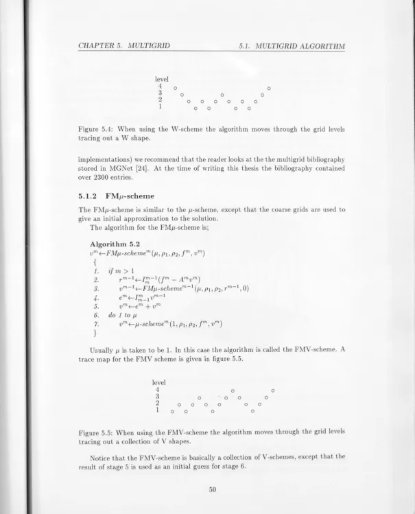
5.4

5.5

5.6

5.7 5.8 6.1 6.2 6.3

6.4

6.5

6.6

6.7

6.8 6.9 6.10 6.11 6.12 6.13 6.14

6.15

6.16 6.17 7.1 7.2 7.3 7.4 7.5

7.6

7.7 7.8

7.9

7.10 7.11 7.12 7.13

.1 .2

EdgeTable structure . . . . Connect Table structure . . . . . Class hierarchy for parallel grid

1 Dimensional grid showing inter-grid connections Ghost nodes used to complete the inter-grid connections V-scheme . .

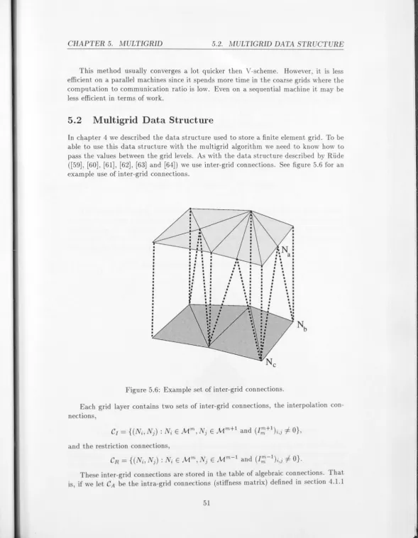
W-scheme . . . . FMV-scheme . . . . Example set of inter-grid connections.

Inter-grid connections from adaptive refinement ConnectTable structure.

Initial Triangulation . .

Triangulation after one refinement sweep. Triangulation after two refinement sweeps

Base edges marking the triangles which need to be split Triangles split independently across the processors Triangles split along the base edges . . . . Two refinement sweeps dividing the grid size by 2 . Steps involved in splitting a triangle . . . . Inter-grid connections for non-adaptive refinement A full node can not be added between two ghost nodes . Processors boundary edges . . . .

ode I.D example . . . . Refinement of quadrilateral grids Refinement of tetrahedral grids .

Refinement algorithm for tetrahedral grids. Example placement of base edges . . . . Example of bad placement of base edges . .

Three levels of refinement of the L-shaped domain

Error after three levels of refinement of the L-shaped domain Error after four levels of refinement of the L-shaped domain The error indicator defines the regions of refinement

Example triangulation with interface-base edges . . . eighbouring coarse grid triangles . . . . Resulting triangulation showing interface-base edges Compatibly divisible triangles . . . . Find the split edge . . . . Example inter-grid connections for adaptive refinement . Defining the interpolation connections

Find_Error_Triangle . . . . Adaptive refinement in parallel

Example load distribution Balanced distribution

LIST OF FIGURES LIST OF FIGURES

8.3 Example movement of nodes 97

8.4 Neighbouring processors . . 98

.5 Example movement record. . 99

8.6 Emigrate movement . . . . . 100

8.7 Example distribution in a ring of processors 101 8.8 Resulting distribution after first iteration of Find_Positive_Movement. 101

8.9 Example distribution of nodes. 102

8.10 Balanced distribution 102

8.11 Actual distribution . . . 102

8.12 Example of islands forming .13 Pick the processors .. .. . 8.14 Example bucket sort . . . .

8.15 Example bucket sort with full bucket 8.16 Example movement of nodes

.17 Moving the nodes .

8.18 Example division . . . A.1 Coarse grid for example 1 A.2 Fine grid for example 1 . A.3 Example division for example 1 A.4 Solution for example 1 .. A.5 Error for example 1 . . . . A.6 Coarse grid for example 2 A.7 Fine grid for example 2 . A.8 Example division for example 2 A.9 Solution for example 2 . . A.10 Error for example 2 . . . . A.11 Coarse grid for example 3 A.12 Fine grid for example 3 .

B.1 Coarse grid for adaptive example 1 B.2 Fin grid for adaptive example 1 . B.3 Example division for adaptive example 1 . B.4 Solution for adaptive example 1 .. B.5 Error for adaptive example 1 . . . B.6 Coar e grid for adaptive example 2 B.7 Fine grid for adaptive example 2 . B. Example division for adaptive example 2 . B.9 Solution for adaptive example 2 .. B.10 Error for adaptive example 2 . .. B.11 oarse grid for adaptive example 3 B.12 Fine grid for adaptive example 3 . B.13 Example division for adaptiv xample 3 . B.14 Solution for adaptive exampl 3 .. B.15 Error for adaptive example 3 . . . B.16 Coarse grid for adaptive example 4

LIST OF FIGURES

B.17 Fine grid for adaptive example 4 . . . B.1S Example division for adaptive example 4 . B.19 Solution for adaptive example 4 . . . .. .

LIST OF FIGURES

Chapter

1

Introd uction

Multigrid methods are fast and powerful methods for solving a wide variety of prob-lems. Many theoretical and practical studies have shown that they offer near optimal efficiency results. However, as with any numerical method, the time taken to solve a problem is limited by the speed of the underlying machine. The aim of this thesis is to present a program which combines the numerical efficiency of the multigrid method with the computational power of a high performance parallel machine.

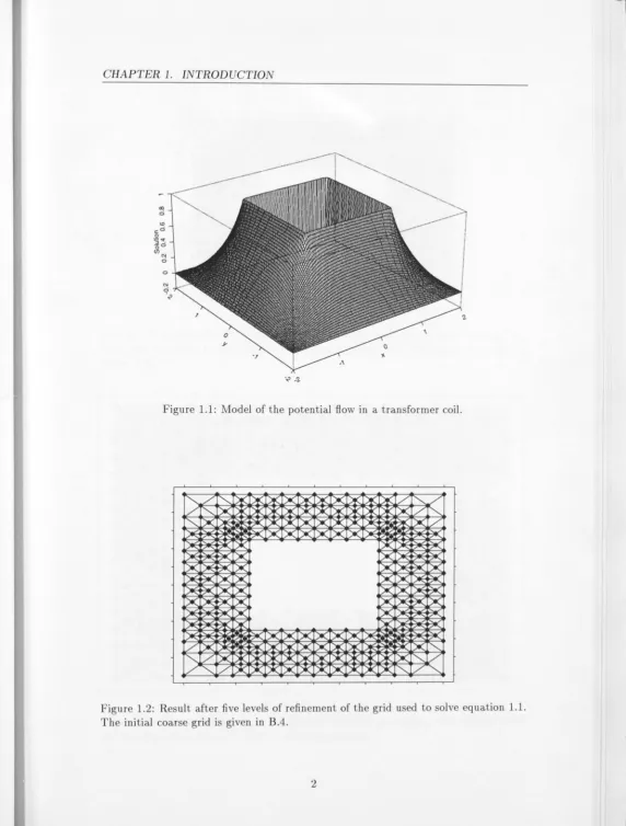
Early experiments with parallel multigrid considered uniform grids on a square domains. However many physical problems are not well modelled by such a structured grid. Consider for example the following problem taken from Collatz [20] which is designed to model the potential flow in a transformer coil by the stream function equation

6.u = 0, (1.1)

with the boundary defined as

u=o

@]

The computational technique used to solve such a problem should put most of the work into those parts of the region where the flow is changing most rapidly, such as the inner corners shown in figure 1.1. Putting extra work into solving the problem in th other parts of the region is not necessary and degrades the performance of the algorithm.

The technique that we use to solve such a problem is the adaptive finite element method. For example, figures 1.2 and 1.3 show how we adapted the grid to obtain the solution given in figure 1.1.

CHAPTER 1. INTRODUCTION

Figure 1.1: Model of the potential flow in a transformer coil.

~/ "-... 1(':'::

_.:.::

X

.:.:: .:.::

X X :::.::: 1( / _~/

/:

~

;-::..

~ ~

::.::

)K

::.::

_X )K

::.c ;;:::,

_KX

/

"-'"

:x

::-::.

:.:

x x

:.:

x

X

/"

1'../ _{"-'" ... X ')e( X X X "X}

)IE; >;;.E _~

y

l /

...,[X [X

"X "5E

~

c:-

IX

)IE; t;.::

_X

~ ~ iX

:.:

IX X r:::-E

~

~ ~

_IX

;-

IX IX

r:::-E

~

X

:::-:

~

l.::-:

X

c:-E ~

X

(X

X

c:-E

;.E ~ l /

"-..C: _{X X X IX} )K )K

/"

x:

.:..:

)K

.:..: :.:

)K

.:..:

X

~

~

/

X

r::.:::

:::+:: ~ X i)e( _{~ :::+::} )K' _{"X ~ '/"} V~ V X X X X X- X X X

_""-

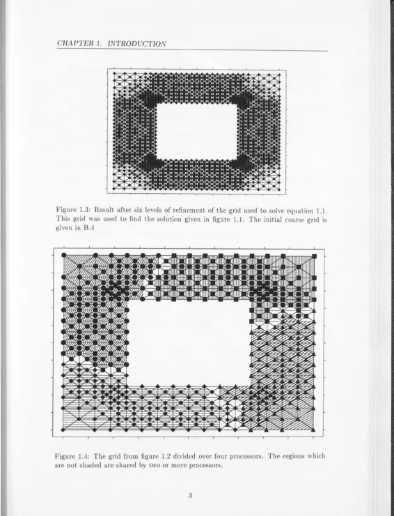
V~

[image:15.629.44.617.13.768.2]

CHAPTER 1. INTRODUCTION

Figure 1.3: Result after six levels of refinement of the grid used to solve equation 1.1. This grid was used to find the solution given in figure 1.1. The initial coarse grid is given in B.4

[image:16.630.56.623.18.759.2]

CHAPTER 1. INTRODUCTION _{1.1. PROGRAM DESCRIPTIO}

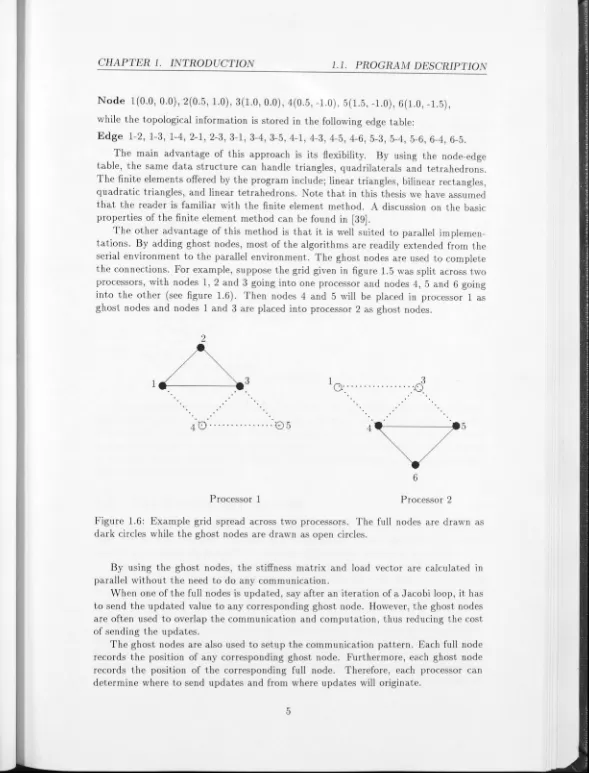
The unique feature with the implementation presented here is that our data

struc-ture stores unstrucstruc-tured grids. For example, figure 1.4 shows the grid from figure 1.2

spread over four processors. The regions which are not shaded are shared by two or more processors.

By using such a method we are able to solve problems on a wide variety of domains using different shaped grids. Furthermore, all of the work may be done on the

proces-sors, except for defining the initial coarse grid. That is, the refinement, the multigrid solution and the load balancing are all computed in parallel thus offering a flexible high performance algorithm.

1.1

Program Description

The program is designed to solve linear elliptic partial differential equations of the form

auxx

+

2buxy

+

CUyy

+

dux

+

euy

+

fu =

G(x,

y)

defined on two dimensional polygonal domains. The coefficients a, b, c, d, e, f are real valued constants, while G(x, y) is a real valued function. To ensure that the equation is elliptic we assume that ac

>

b2_.

We also consider a three dimensional example of the form

.0.u

+

fu

=

G(x,

y, z),

on the unit cube.

J n both cases the boundary condition are Dirichlet.

2

1 __ - - - - -__ 3

---_

5

[image:17.629.50.620.18.764.2]

6

Figure 1.5: The grid is stored in a node-edge data structure. The node table holds the

geometrical information while the edge table holds the topological information

CHAPTER 1. INTRODUCTION _{1.1. PROGRAM DESCRIPTIO}

Node 1(0.0,0.0),2(0.5,1.0),3(1.0,0.0),4(0.5, -1.0),5(1.5, -1.0),6(1.0, -1.5), while the topological information is stored in the following edge table:

Edge 1-2, 1-3, 1-4,2-1,2-3,3-1,3-4,3-5,4-1,4-3,4-5,4-6,5-3,5-4,5-6, 6-4, 6-5. The main advantage of this approach is its flexibility. By using the node-edge table, the same data structure can handle triangles, quadrilaterals and tetrahedrons. The finite elements offered by the program include; linear triangles, bilinear rectangles, quadratic triangles, and linear tetrahedrons. ote that in this thesis we have assumed that the reader is familiar with the finite element method. A discussion on the basic properties of the finite element method can be found in [39].

The other advantage of this method is that it is well suited to parallel implemen-tations. By adding ghost nodes, most of the algorithms are readily extended from the serial environment to the parallel environment. The ghost nodes are used to complete the connections. For example, suppose the grid given in figure 1.5 was split across two processors, with nodes 1, 2 and 3 going into one processor and nodes 4, 5 and 6 going into the other (see figure 1.6). Then nodes 4 and 5 will be placed in processor 1 as ghost nodes and nodes 1 and 3 are placed into processor 2 as ghost nodes.

2

1 __ - - - - -. 3

1

0·.···

..

0.

3

4

·6···

:05

4.---~.5

6

Processor 1 Processor 2

Figure 1.6: Example grid spread across two processors. The full nodes are drawn as dark circles while the ghost nodes are drawn as open circles.

By using the ghost nodes, th tiffness matrix and load vector are calculated in parallel without the need to do any communication.

When one of the full nodes is updated, say after an iteration of a Jacobi loop, it has to send the updated value to any corresponding ghost node. However, the ghost nodes are often used to overlap the communication and computation, thus reducing the cost of sending the updates.

[image:18.629.38.627.17.790.2]

CHAPTER 1. INTRODUCTION _{1.2. MULTIGRID METHOD}

1.2 Th

e

Multigrid M

e

thod

As the name suggests, multigrid methods use multiple layers of grids. The idea being that each grid layer contributes different pieces of information towards the solution of the problem. In terms of elliptic partial differential equations each grid layer is used to

remove different frequency components of the error.

There are many variations of the multigrid theme, but as an example lets look at the V-scheme. Given a nested sequence of grids, Ml C M2 C ... C Mn , the algorithm for the V-scheme is;

Algorithm 1.1

vm f--V-schemem (Pi, P2,

f

m, vm)

{

}

do 1 to Pi

vmf--Rm(jm _ AmvID )

ifm> 1

rID - 1f--l;::-1(jID _ AIDvID )

VID-1f--V-schemeID-1 (Pi, P2, r ID - 1,

0)

eIDf--l;::_l vID -1

vIDf--eID

+

v ID

do 1 to P2

vmf--RID(jID _ AIDvm )

The most frequently used relaxation methods, RID, are weighted Jacobi or Gauss-Seidel, but these are not the only ones that may be used, for example red-black or line Gauss-Seidel are also often used. The interpolation operator, 1;::_1' used in this report

is linear interpolation. The restriction operator, 1;::-1, is defined to be the transpose of the interpolation operator. See Briggs [14] for further discussions on the philosophy

behind the multigrid method.

1.3 The Parallel Environm

e

nt

The program descri bed here was originally developed on a network of S workstations

using the parallel programming language PVM (Parallel Virtual Machine). It was then

ported across to the Fujitsu AP1000 parallel computer for performance testing.

Th main r ason for using a parallel programming language such as PVM as opposed to using native communication paradigms is to increase the portability of our code. A

related, reason is that workstations can be used to test the logic of the program. Once convinced of correct logic, the program may be moved across to a parallel machine for

performance d bugging.

The parallel machine used to test the performance of the program was the AP1000. Th AP1000 is an experimental machine from Fujitsu. The machine at the Australian ational Univer ity has 128 cells, consisting of a SPARe chip, arranged in a two dim en-sional torus format. One of the main features of the AP1000 is its good communication

broad-CHAPTER 1. INTRODUCTION _{1.4. REFINEMENT}

casting), S-Net (synchronisation) and T-Net (torus or point-point). By using the three networks, conflicts between the three different types of communication is eliminated.

1.4 Newest Node Refinement

The initial coarse grid is defined on the host machine. Once it has been spread across the processors it is refined further by using the newest node bisection method ([54], [55] [56]). To refine triangular grids this methods splits the triangles at the edges which sit opposite the newest node. For example suppose the centre point in figure 1.7 is the newest node, then the resulting triangulation after one and two levels of refinement are shown in figures 1.8 and 1.9 respectively.

Figure 1.7: Initial triangulation. The dark circles represent the newest nodes.

Figure 1. : Triangulation after one refinement sweep. The dark circles represent the newest nodes.

[image:20.629.33.616.19.767.2]

CHAPTER 1. INTRODUCTION

1.5. LOAD BALA

CE

The advantage of this method is that the angles are guaranteed to be bounded away from 0 and IT (see [54]).

To find the regions of refinement we use an error indicator similar to the one used by Mitchell ([54], [55] and [56]) and Riide ([62]). Roughly speaking the program picks the triangles to refine by looking at how well the coarse grid approximates the solution on the fine grid. That is, if node i is the midpoint of an edge in grid Mm then the error indicator assigned to the edge is

(1.2) where

To refine the grid adaptively we split the triangles along the edges whose error indicator is greater than a given tolerance.

During adaptive refinement it may be necessary to refine some of the neighbouring triangles to keep the angles bou nded away from 0 and IT. To keep track of these neigh-bouring edges in parallel we introduce interface-base edges. Interface-base edges are base edges which sit between two different levels of refinement. For example, suppose we wanted to split the triangle in figure 1.10 along the interface-base edge 11, then we must split the base edge B7 first. Note that several neighbouring triangles may have to be split, so the refinement may travel over several processors.

Figure 1.10: Example triangulation with interface-base edges 11 and 12 and base edges B3, B4, B5, B6 and B7. The base edge B7, should be refined before the interface-base edge 11.

1.5 The Load Balance Method

CHAPTER 1. INTRODUCTION _{1.5. LOAD BALANCE}

Level

II

Processor Number

1 2 7 8

0 3 3 3 3 3 3 3 3 1 12 10 9 8 9 10 9 5

2 13 12 10 8 9 11 11 6

3 15 15 12 9 11 14 13 7

4 83 56 64 75 78 60 58 38

5 267 234 299 279 278 242 234 147

Table 1.1: Number of nodes per processor after adaptive refinement of the grid used to solve equation 1.1 without balancing the load. Level 0 is the initial coarse grid.

5

1) 2)

2

0

6

3 3

Figure 1.11: Example movement of nodes.

To re-balance the load we let the nodes 'flow' out of the processors with too many nodes into the processors which do not have enough. By flow we mean that the nodes follow the edges between neighbouring processors. The algorithm consists of the fol-lowing four steps;

1. Balance the number of nodes.

2. Pick the nodes to be moved.

3. Pick the processors. 4. Move the nodes.

1.5.1

Balancing The Numbe

r

Of Nod

e

s

CHAPTER 1. INTRODUCTION _{1.6. OVERVIEW}

1.5.2

Pi

c

king

W

hich

N

od

es T

o

M

o

ve

The next step is to pick which nodes should be moved. The main aim here is to find the nodes in such a way that the grids are not split up into lots of little segments. The ratio of ghost nodes to full nodes is high for these segments so they increase the amount of communication to computation. The nodes that we pick are those nodes that are sitting on the boundary of the processor and are not connected to many other nodes.

1.5.3

Pi

c

king The P

r

oc

ess

o

rs

Once we have determined which nodes are to be moved, we then need to find which processor they should be moved to. To do this we use the Kernighan-Lin method. The Kernighan-Lin method assigns to each node a preference value. The preference value compares the number of connections between the current node and the nodes in the neighbouring processors. The node is moved to the processor which has the highest preference value so as to reduce the number of communication links.

1.

5.4 M

o

v

ing

T

h

e N

od

es

One of the more difficult parts of the algorithm is moving the nodes, as we have to be careful to update the data dependencies correctly. The method that we use is to make a record of intended movement, communicate that information and then move the nodes. That way the program can freely move the nodes, without the need to send their new positions to the corresponding ghost or full nodes, and then use the movement records to update the communication pattern.

1.6

Ov

e

rvi

e

w

The remainder of the thesis has been broken up into eight chapters which roughly match the sections described above.

Chapter 2 gives some technical details. The program is written in a mixture of C++ and PVM. We chose a high level language such as C++ because it offers a good envi-ronment for the development of an experimental program. The parallel programming language PVM was chosen to increase the portability of the code. The program was originally developed on a network of

SU

workstations and then ported across to the Fujitsu P1000 for performance testing.

Chapter 3 gives an overview of the parallel implementations of multigrid methods which use structured grids. We start the chapter by focusing on the model problem of Poisson's equation on a square domain. This problem highlights many of the features of the parallel implementation of multigrid, including the observation that if the problem size is large enough then the loss in efficiency due to idle processors is negligible. We finish the chapter by giving a brief description of other packages which are designed to handle adaptive grids.

CHAPTER 1. INTRODUCTION _{1.6. OVERVIEW}

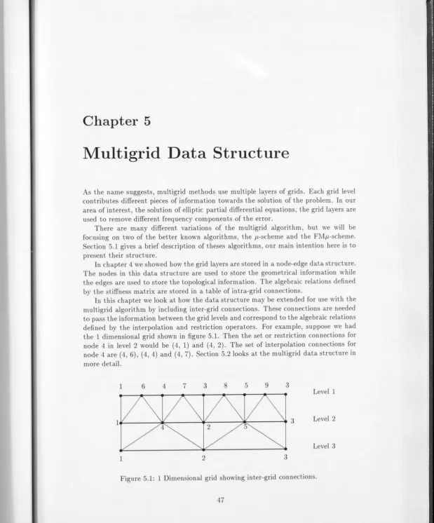
Chapter 5 extends the nodes-edge data structure so that it can be used by the multigrid algorithm. The interpolation and restriction operators are defined by a set of inter-grid connections.

Chapter 6 describes the non-adaptive refinement routines. We have defined routines which may refine triangular, quadrilateral and tetrahedral grids. The methods that we use are based upon the newest node bisection method. The triangle and quadrilateral grids may be split in parallel without any communication*. The tetrahedral grids do need the values of the boundary edges to be updated after each refinement sweep, but the communication and computations have been overlapped to reduce the cost.

Chapter 7 addresses the problem of adaptive refinement of triangular grids. When a triangle is refined some of the neighbouring triangle may also have to be split to keep the angles bounded away from 0 and 7r.

In

the parallel implementation, these neighbouring

triangles may be sitting on other processors. We show how to use interface-base edges to keep track of the neighbouring triangles.

Chapter 8 presents the algorithm used to re-balance the load. During adaptive refinement the work may be unevenly distributed across the processors. To re-balance the load we let the nodes flow out of the processors with too many nodes into the processors which do not have enough.

Chapter 9 concludes our discussion. We briefly review the results and mention some possible future projects.

Chapter

2

Programming Environment And

Algorithm Notation

The multigrid program presented in this thesis is written in a mixture of C++ and the parallel programming language PVM.

C++ is an object orientated programming language. The difference between an object orientated language and a normal procedural language (such a

C)

is that the definition of a record must be accompanied by the set of operations which may be performed on it. The object given by the record and its associated operations is called a class in C++.

The internal representation of the record is usually hidden from the users of a class,

access may only be obtained through its operators or members. Consequently, the method used to store the information can be readily changed without effecting the rest of the program. Therefore, it is fairly easy and safe to experiment with new ideas and different approaches.

One of the major benefits of an object orientated language is that the external view of a class is limited to the definition of its operators, so the user can concentrate on the classes semantics not its syntax.

PVM (Parallel Virtual Machine) is a public domain parallel programming language which is available on a wide variety of platforms.

It

offers a set of communication calls which are independent of the underlying machines architecture. Using such a language increases th portability of the code. Most of our developmental work was done on a network of SU workstations, the program was then ported across to the Fujitsu AP1000 for p rformance testing.

The AP1000 is an experim ntal machine from Fujitsu. The machine that we have at the Australian National University has 128 processors arrang d in a two dimensional torus format. It uses three different communication networks to avoid conflicts between the different types of communication.

CHAPTER 2. PROGRAMMING ENVIRONMENT 2.1.

c++

2.1

C

++

The final prod uct presented here hides many of the different approaches that we have

tried. aturally, this is not unique to any project of this size, so the program had to

be written in a language which can readily accommodate any changes. For this reason

we decided to use C++.

2.1.1

Advantages

of

C

++

C++ is an object orientated programming language. The use of C++ classes allows the

program to be written in a manner which is intrinsic to the underlying mathematical

problem. That is, a user familiar with the notation of finite elements should be able to

use the program without getting lost in the details of the data structure. As an example,

the code given in figure 2.1 defines a linear polynomial on a triangular element. Even

though we have only given one line descriptions of the operators we feel that their

meaning is self explanatory.

otice that the members of the class are divided up into two sections, public and

private. Other parts of the program may only access information about the polynomial

through the public members. For example, to evaluate the polynomial at a given point the evaloperator must be used, as the coefficients consLcoeff, x_coeff and y_coeff may not be accessed directly.

This information hiding is one of the best features of C++. It means that a class may

be used without knowing the details of the data structure. It also implies that the data

structure may be readily changed. For example, we could change LinearPolynomial so that the co fficients are stored in an array, however, this would not affect the rest of

the program since it does not change the definition of the public member functions.

C++ also has some other useful features, such as operator overloading, inheritance, templates and default initialisers. These are described in more detail in the multitude of books on C++ such as [15], [36] and [45]

2

.

1.2

A

lgori

thm Notation

We have presented the algorithms in this thesis in a style similar to the classes used in

C++. For example, to find the value of a node in C++ we would use;

node.geLvalueO;

In our algorithm environment we use

node. value

These algorithms are not intended to be literal translations of the code. Statements

like

table

+-

table U {node}

are likely to be implemented in

++

as

if (! lable. is-in ( node))

table. add_node( node);

CHAPTER 2. PROGRAMMING ENVIRONMENT

class LinearPolynomial: public TrianglePolynomial

private:

I I

P

=

aDO

+

a01x

+

alOy

Real consLcoeff; Real x_coeff;

Real y_coeff;

public:

II

aDO

II

aID

II

aOl

I I

constructor: set the coefficients to zero

LinearPolynomialO;

I I

copy constructor

LinearPolynomial( const LinearPolynomial &poly);

I I

destructor -LinearPolynomialO;

I I

set aDO

inline void seLconsLcoeff(Real coeff){ consLcoeff

I I

set aID

inline void seLx_coeff(Real coeff){x_coeff coeff;}

I I

set aOl

inline void seLy_coeff(Real coeff){y_coeff coeff;}

I I

get aDO

coeff;}

inline Real geLconsLcoeffO const {return consLcoeff;}

};

I I

get aOl

inline Real get...:LcoeffO const {return x-coeff;}

I I

get alO

inline Real geLy_coeffO const {return y_coeff;}

I I

evaluate the polynomial at the position (x, y)

Real eval( Real x,

Real y) const;

I I

djfferentiate the polynomial wi th re p ct to X LinearPolynomial dxO const;

I I

djfferentiate the polynomial with respect to y

Lineal'Polynomial dyO const;

2.1. c++

Figur 2.1: Example C++ code. This class defines the linear polynomials on a triangular element.

10

20

30

40

CHAPTER 2. PROGRAMMING ENVIRONMENT 2.2. PVM

2.1.3

Di

s

ad

v

antag

es

of

C++

To be fair we should mention some of the disadvantages of C++.

Some authors argue that a problem with C++ is that it is slower than C (see for example [23]). However there are several options available to increase the speed of C++. These include the use of inline functions. In an inline function the procedure call is replaced by the body of the procedure during compilation, thus removing the cost of calling the function. This is similar to a #define in C except that type checking is performed on in line functions. Another approach is to write the expensive numerical parts of the code in another language such as C or Fortran. See, for example the codes written by Baden et al. (section 3.3.3) and Quinlan (section 3.3.4).

For a thorough discussion on the problems with C++ see Joyner [40]. Many of Joyner's arguments against C++ rest on the fact that it is built upon C. Joyner points out that C++ can never be a true object orientated language since it uses features from a language which is not object orientated. For example, it would be difficult to add garbage collection to C++ and still keep it compatible with C (section 3.24, [40]). A true high level language should have garbage collection to avoid the bugs that often arise when manipulating memory in C.

Many of Joyner's arguments are valid, C++ is not perfect. However, we feel that with a disciplined programming style, the user can exploit C++'s high level constructs and obtain reasonable performance results.

2.2

P

ara

llel Environ

me

nt

To obtain optimal performance from a parallel machine it is necessary to tailor the code to the underlying architecture. Theses modifications are usually very specific and can not be carried across from one machine to another. For this reason we have decided to use a parallel programming language such as PVM.

Another important benefit of a parallel programming language is that the code can be developed on a network of workstations. We wrote and debugged the multigrid program on a network of SUN workstations. We found that this method was preferable to writing the code from scratch on a parallel machine since the resources on the workstations are more freely available, easily accessed and cheaper.

Naturally, the workstations do not offer the performance available on a parallel machine, so the program was ported to the APlOOO for performance testing.

The program that we developed is independent of the architecture of the machine. Neighbouring processors are defined by the node-edge data structure not their physical location. However, this does rely on some underlying assumptions about our commu-nication model. The primary assumption we make is that the communication time is not d pendent upon the length of the communication path, we would not expect good performance on a machine such as the Hypercube. However, we believe that our package would be well suited for more modern architectures such as the T3D or CM5 where the time is not dependent upon the communication length.

CHAPTER 2. PROGRAMMING ENVIRONMENT _{2.3. APlOOO}

with another parallel programming language, only the private member functions have to be changed. We would like to try a version which uses MPI as it has many useful features not available in the current version of PVM. These features include global operations such as global sums and global maximums.

2.3

APIOOO

The APlOOO is a distributed memory MIMD machine. It contains 128 processors (or cells) which are combined to form a Cellular Array Processor (so it is also known as the CAP). The machine we have on campus is a single user machine.

One of APlOOO's most powerful attributes is its low communication times. It uses

three different interfaces to avoid conflicts between the different message types. They are the B-net, S-net and T-net. The B-net is used for broadcasting and communication between the processors and host. The S-net implements barrier synchronisation. The T-net, or torus network, gives point-to-point communication between neighbouring processors. Each processor is connected to it's four nearest neighbours in a 2D torus network.

The APlOOO processors' use a 25 MHz SPARC chip and have 16 megabytes of dynamic (RAM) memory. For further information see [1], [2], [29], [35] and [38]. Some

Chapter 3

Development Of Structured

Multigrid

The use of multigrid methods on serial machines has proven to be an effective way of solving a wide range of problems. But how well does multigrid perform on parallel machines? The need to sequentially move down the grid levels and problems with idle processors might give one the impression that multigrid methods are inherently serial. However many studies have proven that even standard multigrid algorithms give good efficiency results. This chapter gives a historical overview of the development of parallel multigrid, in particular in the case of structured grids.

Our discussion shall initially focus on the model problem of Poisson's equation on a square domain. We will show that if the problem size is large enough then the loss of efficiency due to the idle processors which arise during the coarse grid iterations is negligible.

For massively parallel machines, however, the problem size may have to be fairly large before we see the desired efficiency results. In the second part of this chapter we shall present some variations of the standard multigrid method which are designed to keep all of the processors busy during the coarse grid iterations. These methods include the U-scheme and FMU-scheme, Parallel Superconvergent Multigrid, Filtering, Frequency Decomposition and Domain Reduction. The approach taken by Parallel Superconvergent Multigrid, Frequency Decomposition and Domain Reduction is to use multipl coarse grids so the total numb r of nodes does not decrease as we move down the grid levels. The Filtering algorithm works on the fine and coarse grids at the same time. The U-scheme avoids idle processors by not moving down to those coarse grids which have less nodes then processors.

aturally, not all problems may be modeled by Poisson's equation on a square domain. Some parallel implementations of multigrid which have been designed to

CHAPTER 3. STRUCTURED MULTIGRID 3.1. MODEL PROBLEM

We have taken a different approach. Our underlying data structure is unstructured. We feel that an unstructured data structure is better suited to the dynamic nature of many physical problems, such as flow problems.

3.1

Model Problem

Many experiments with parallel multigrid have focused on the model problem

6..u

f

in

n

u 0 on

an,

where

n

is the unit square domain.

We shall start our background description with this model problem since it high -lights many of the properties of parallel multigrid.

As a specific example we will refer to a multigrid algorithm we developed on the Fujitsu API000. The API000 is a distributed memory MIMD parallel machine. It is described in detail in section 2.3, but the main feature that we would like to highlight is that it uses a 2D torus topology and its communication speed is not dependent upon the length of the communication path.

3.1.1

The Standard Multigrid Algorithm

We shall first cover the unit square domain with a uniform grid

Mm

=

(ih

m,

jh

m

)

o

<

i, j

<

2m

, hm

=

2!"

and use the 5-point star method is used to form a discrete approximation to the model problem.

To solve the system of equations we use the multigrid algorithm given in section 1.2. The benefit of using such a standard multigrid algorithm is that it is supported by many theoretical studies.

The relaxation methods used here tend to be Jacobi or Red Black Gauss-Seidel ([13], [16], [17], [37], [47]). Exam pie inter-grid operators include bilinear interpolation, full weighting restriction and injection ( [13], [37], [47]). All of these operators may be calculated in parallel and only need to use local updates.

In our implementation we used block partitioning as described in the next section. However, on hypercube type of architectures where the communication time is depen-dent upon the communication length Gray codes are often used. By assigning the nodes to the processors in the order given by a binary reflected Gray code the distance between neighbouring grid points will remain constant as we move down the grid levels. For example, if a 1 dimensional mesh is mapped onto a cube using a binary reflected Gray code then the distance between neighbouring nodes on the fine grid is one, while the distance for the nodes on the coarse grids is two. See for example [16] and [18].

3.1.2

Block Partitioning

CHAPTER 3. STRUCTURED MULTIGRID

J!1

Q;

u ~ ~ c :>

o

m

""

_"

...J

Top Boundary Cells

BoHom Boundary Cells

3.1. MODEL PROBLEM

Figure 3.1: Domain decomposition. This diagram shows how a grid of size h = 1/24 _is

divided amongst the processors.

may be done using a machine such as the API000 whose architecture resembles an

array of cells.

Each block is usually surrounded by an overlap region as in figure 3.2. These

regions contain nodes from the boundary of the neighbouring processors. The main

advantage of this approach is that the serial code may be easily extended to the parallel

environment. All of the multigrid operations mentioned in the previous section only use local information. For example, to calculate the current value at a given node,

(i

,

j

),

using the five-point star method, we only need values from the surrounding nodes,

(i+l,j)

,

(i-l,j), (i

,

j+l)

and

(i,j-l).

The inclusion of the boundary layer ensures

that that information is available (see figure 3.2).

In our implementation on the API000 we stored the updates in a communication

buffer which is similar to the ghost nodes used in the unstructured grids (see section

4.2.1).

Th only complication in the parallel implementation is the need to keep the values

in the overlap region up to date. However since we are using structured grids the

information can be communicated in a systematic way. In our implementation on the

CHAPTER 3. STRUCTURED MULTIGRID _{3.1. MODEL PROBLEM}

Cell

Overlap Region <:;)···0···0···0···0-···0

Ifl--:I---:r:I]I

: :: : Grid Block : :: :

n

t

--l]-:lf;

0

···

.

···

6

···

6

···

6

···

6

Figure 3.2: The grid blocks are usually surrounded by an overlap region. This ensures that the information needed by the multigrid algorithm is accessible.

Send updates to the lell Send updates to the right

Send updates to the top Send updates to the bottom

Figure 3.3: To update the overlap regions the processors send their boundary values to

CHAPTER 3. STRUCTURED MULTIGRID _{3.1. MODEL PROBLEM}

their right neighbours, then their top neighbours and finally their bottom neighbours. See figure 3.3. This avoided any communication conflict on the network. Briggs et. al [13J also use this method.

3.1.3 Coarse Grids

The nodes in the coarse grids are usually taken to be the even numbered nodes from the fine grid (see figure 3.4). As the algorithm moves down the grid levels we may find that the number of nodes has decreased so much that there are more processors then nodes. These lower grid levels are the main bottleneck in the parallel implementation of multi-grid methods since they do not contain enough nodes to keep all of the processors busy. Furthermore, as we move down the grid levels the length of the communication paths may start to increase, which increases the communication time on some architectures.

Grid at level m = 4 (Iinest grid)

j---e- - -_I'i'---Q. -- - - i J I

I

I I

I

I

I

I

r-

Q

-I

Q- - - --Q

I

_I

_I

I

_i

I

_I

r

---Q.-.-.---_~----

r-j

I

I

I

' _I I _I

()-

-r---

t-

-

-

---

r----l

I

I

I

I

(J- - --.Q._---_{1&-- -}a - - - a

.. e

!

~b

_.

_!

c r -I

I

I

I

I <>---_I

I

!

I

I

--I

".--r-

T

-

-r-

i

i

T

j I j I i i I

····I~ I I !

Grid at level m = 3

- - -~---~--<>

I

I

I I

I

I

I

_I

I

1

I

_I

j

!

I !

I

I

_I

I

- - -1<>- -

--Grid at level m = 2 Grid at level m = 1 (coarsest grid)

Figure 3.4: Moving down the grid levels. For m contain any grid points are inactive.

1, the processors which do not

CHAPTER 3. STRUCTURED MULTIGRID _{3.1. MODEL PROBLEM}

On the AP1000 the communication time is not dependent upon the communication

length, therefore we left the coarse grid nodes in the same processor as the corresponding fine grid nodes.

Section 3.2 looks at some modifications of the standard multigrid method which are designed to avoid the problem of idle processors.

3.1.4 Efficiency Results

For

The Parallel Implementation Of

Multi-grid

Despite the idle processors, multigrid methods still give good efficiency results because the proportion of time spent in the fine grids is higher than the time spent in the coarse grids. Therefore, if the number of grid levels is high enough then the loss of efficiency due to idle processors is negligible.

To back up these arguments we have some results from the AP1000. Figure 3.5 shows the efficiency results for the multigrid method given in algorithm 1.1. The separate readings for the same number of processors is due to different processor con-figuration. For example, 4 processors can be configured as a 1 x 4, 2 x 2 or 4 X 1 array. ~

"

., c;; >- <D U

c: 0

..

'u rD

..

0 N 0 0 0 2

Time study for mu1

=

3, mu2

=

2 (Vscheme)

I

~

o

"

II

"

I

°06

~

:

:

I

n"" 10

8 16 32 64

Number of processors

8 o o

"

II 128

Figure 3.5: Efficiency results for V-scheme obtained on the AP1000 using single preci-sion op rations. n = the number of levels of refinement

ot that for 10 and 9 grid levels the graphs show efficiency values greater then

1. These sup r-efficiency results are a consequence of memory cache effects. When a large grid is placed on 1 processor it uses a lot of the proces or's memory. In fact, we wer unable to solve the model problem on 1 processor using 10 grid levels and double

CHAPTER 3. STRUCTURED MULTIGRID 3.2. PARALLEL MULTIGRID

processors, say 2, then a higher proportion of the grid will sit in the processors high

speed memory (or cache). Therefore, the time taken to do the computations for the 2 processor case may be less than half of the time taken to do the computations with

1 processor. If this reduction is greater then the increased communication costs the efficiency will be greater than one.

In figure 3.5 we see that the efficiency drops off as more processors are added. When there is a large number of processors the number of nodes per processor is quite small so more processors are idle for a longer time.

Another feature that figure 3.5 highlights is that as the number of grid levels in-creases so does the efficiency. Increasing the number of grid levels decreases the

pro-portion of time spent in the coarse grids. If the problem size is large enough, then the

loss in efficiency due to idle processors may be so small that it can be disregarded.

These efficiency results have also been observed by other authors ([13], [18], [47]).

3.2

Modifications To Standard Multigrid

We mentioned previously that we often get idle processors when doing the computations on the coarse grids. We also postulated that if the problem size is big enough then the loss in efficiency is negligible. However, on a massively parallel machine it may not be

possible (or practical) to fit a big enough problem on the machine to get the increased

efficiency results. In this section we present some variations of the standard multigrid

method which are designed to avoid the idle processors.

ote that care must be taken when using these methods since they no longer sit in the theoretical framework of standard multigrid. For example Douglas [22] points out that in the Parallel Superconvergent Method we may find that we are computing the corrections in one of the correction spaces, while the corrections in the remaining spaces add up (pointwise) to zero.

3

.

2.1

V

-scheme and FMV-scheme

CHAPTER 3. STRUCTURED MULTIGRID

Algorithm 3.1

vffi f-U-schemeffi(Pi' P2, fffi, Vffi)

{

}

do 1 to Pi

Vffif-Rffi(jffi _ Affivffi)

ifm>

c

rffi-if-I;:::-i(jffi _ AffiVffi)

Vffi - i f-U-schemeffi - i (Pi, P2, rffi-i, 0)

effif-I;:::_i Vffi- i

vffif-effi

+

v ffi

do 1 to P2

vffif-Rffi(jffi _ AffiVffi)

3.2. PARALLEL MULTIGRID

The problem with this approach is that we loose the information from the coarse

grids so the convergence rate deteriorates.

3.2.2

Filtering

The filtering algorithm ([66]) is similar to standard multigrid except that two correction

equations are formed after the relaxation step, one for the high frequency components

and one for the low frequency components. The subproblem associated with the high

frequency components is solved by using g relaxation sweeps on the fine grid while the

other su bproblem is solved by using coarse grid correction as with standard multigrid.

In this method the number of nodes per processor still decreases as we move down

the levels, but the fine grid relaxation sweeps may be performed in parallel with the

coarse grid correction step.

3.2.3

Parallel Superconvergent

Multigrid

The Parallel Superconvergent Multigrid (PSMG) method ([19], [21], [27], [28], [47]) is

built upon the idea of looking at the fine grid as a collection of coarse grids. That is, instead of just using the even numbered nodes for the coarse grids, the PSMG methods creates two coarse grids, one for the even numbered nodes and for the odd numbered

nodes. Since the total number of nodes is not reduced as we move down the grid levels,

we do not get any idle processors.

If an appropriate relaxation method is chosen the extra information from the second

coarse grid can be exploited to give convergence rates better than standard multigrid.

3.2.4 Frequency Decomposition Method

The fr quency decomposition method ([5], [6], [32]) was developed for use with an

anisotropic equation. This method uses four different coarse grids. They are the

stan-dard coarse grid, the standard coarse grid shifted by h

(= gr

id size) in the x direction,

the standard coarse grid shifted by h in the y direction and the standard coarse grid

CHAPTER 3. STRUCTURED MULTIGRID 3.3. ADAPTIVE METHODS

coarse grids contain different frequency components. For example the operator pro-jected down onto the coarse grid shifted by h in the x direction will contain oscillatory components in the x direction.

Once again, the information from the extra coarse grids may be used to increase the convergence rates.

3.2.5

Domain Reduction

The domain reduction algorithms presented in [12], [22], [25] and [26] use a multilevel approach. That is, the domain is broken up into several regions with the solution on each region being calculated in parallel. The restriction operators on each of these regions are chosen so that they annihilate functions which have certain symmetries and antisymmetries properties. In [26] Douglas and Smith give example operators which lead to a four way decomposition. Brezzi et al [12] give example restriction operator which leads to an eight way decomposition of a square into squares, rectangles and triangles.

3.3

Adaptive Methods

We now direct our attention towards some packages which have been designed to handle more general problems and allow adaptive refinement of the grids. In all of these packages the regions are viewed as a composition of structured grids. Structured grids have several advantages such as; simplified data structures, structured communication and better vectorisation.

LiSS ([58]) is designed to solve systems of nonlinear partial differential equations

Lu = 0,

on a general 2D domain

n

together with some boundary conditions on

an.

It can also solve the corresponding time dependent equation

Ut

=

Lu.

The solution processes is broken up into the following stages,

Pre-processing Definition of geometry, block structure and grid generation

Multigrid solver Parallel solution of equation on structured grids.

Post-processing Graphical visualisation.

The pre and post processing s ctions use sequential codes and must be run on a sequential rna hine.

CHAPTER 3. STRUCTURED MULTIGRID 3.3. ADAPTIVE METHODS

rectangular, boundary fitted grid. The grid is then split further before it is mapped onto the processors.

Once the blocks have been spread across the processors the equation is solved by using the multigrid method. The discretisation method used here depends upon a compact nine-point stencil given by the user.

Further refinement of the grid is given on the host machine. That is, in each block the user determines an areas in which a locally refined grid should be introduced. A new block structure is then built and mapped onto the processors.

3.3.2 Keyser and Roose

Another parallel multigrid implementation is described by Keyser and Roose

[41]

.

The method that they use is similar to the one used in LiSS. That is, they block partition the data, spread the blocks across the processors and then obtain a current approximation. Based upon that approximation the adaptively refined grid is constructed. In order to keep a good load balance the grid is then re-distributed across the processors.

The paper

[41]

focuses on the cost of distributing a multigrid algorithm. In order to distribute the data, the inter-grid and intra-grid data dependencies need to be taken into account. Keyser and Roose looked at several variations of a hierarchical recursive bisection method. These included versions which just re-mapped the fine grids and those which re-mapped both the fine and coarse grids. They found that it was not worthwhile re-mapping the coarse grid levels.

3.3.3 LPARX

The LPARX package developed by Baden et.al

([3],

[42]

,

[43]

,

[44])

was not solely designed for use with multigrid methods. However, it has been used to develop some adaptive multigrid programs.

LPARX supports block-structured, irregular decomposition of the grids. It contains three basic abstract data types, Region, Grid, XArray. The Region is an array index-space which lets the user define the data decomposition. The Grid is an array defined over the Region. It may be of any abstract type such as integers or user-defined types. The XArray is a parallel object which holds the Grids once they have been spread across the processors.

The XArray is intended to represent coarse grain parallelism. Communication between the blocks is controlled by the use of high level copy operations. The actual details of the communication are hidden from the user.

CHAPTER 3. STRUCTURED MULTIGRID _{3.3. ADAPTIVE METHODS}

3.3.4

AFAC

and AFACx

The package developed by Quinlan ([52], [53], [57]) uses the asynchronous fast adaptive composite grid methods, AFAC and AFACx (see also [50], [51] and [52]). The use of such a multilevel approach allows independent processing of the individual grid levels which make up the composite grid.

Let

Ml

C

M2

c ...

c

M n be a nested sequence of grids so that the composite grid

M

C

is defined by

M

C

=

Ui=lM

i.

As with the standard multigrid algorithm we need some discrete operator, Am, an

interpolation operator,

I;",

and a restriction operator,

I

;:'.

An important feature of the AFAC and AFACx algorithms is the use of restricted

grids Mm

=

M:

n

Mm-l.

These grids also ha~e a discrete operator, Am, an

interpo-lation operator,

I

;",

and a restriction operator,

I

;:'

.

Then the AFAC algorithm is;

Algorithm 3.2

vC +-AFAC(r, vC)

{

}

for m E {I, ... , n}

fm+-I;:'(r - ACvC)

for mE {2, ... , n} Jm+-~m(fc _ ACvC)

for m E {I, ... , n}

vm+-o

for mE {2, ... , n} vm+-O

forallmE

{l,···,n}

vm+-(Am)-l fm

if

(m

>

1)

vm+-(Am)-l Jm

for mE {2, ... , n} um+-Ic v m _ Jc v m

m m

vC+-vc

+

IlVl

+

L~=2 um

The steps vm+-(Am)-l fm and vm+-(Am)-lJm may be calculated simultaneously by using a direct solver or a multigrid algorithm.

The r stricted grids are used to liminate error components common to the coarse and fine grids. The step um+-I;"vm - l;..vm prevents these components from

accumu-lating and amplifying.

As an example consider the composite grid M C

=

Ml

U M 2 shown in figure 3.6 (see [50]). Notice that we have also included the restricted grid M2

=

Ml

n

M2.

In the fi rst two loops from algorithm 3.2 the residual is passed down from M C to M l,

- 2 . 2 (A2)-lf2 1

(Al)-lfl