ON THE SPEED OF LOG TRUCKS
b y
T e r r y B e a t h
T h e s is s u b m i t t e d i n p a r t i a l f u l f i l m e n t o f th e
re q u ir e m e n ts f o r t h e d e g re e o f
M aster o f S c ie n c e ( F o r e s t r y )
i n th e A u s t r a l i a n N a t i o n a l U n i v e r s i t y
Except where specific acknowledgement is given, this thesis is my original work.
The speed of log trucks over selected sections of various roads was measured and the loads carried in hauling wood from the plantations in the
Australian Capital Territory obtained from weigh bridge dockets. Two models were derived to predict the sustained speed of log trucks, and the speed after traversing one hundred and fifty metres of an adverse grade, with respect to road gradient, truck power and gross weight.
The significance of the maximum permitted loads on log trucks is examined in relation to the costs .of hauling wood in the Australian Capital Territory
ACKNOWLEDGEMENTS
I am very pleased to have undertaken a year of postgraduate research at the Department of Forestry at the Australian National University and to again participate in some of the discussions in that Department and in extracurricular activities at the University. I must acknowledge long,stimulating and helpful discussions on data processing, statistics and data analysis with other postgraduate students, in
particular Mr. Jerry Leech and Mr. Gary Archer.
A number of organizations made the study feasible. The
Forestry Commission of New South Wales agreed to my request for leave of absence. The Forests Branch of the Department of the Capital Territory, Canberra, employed me for a short period while I worked on the project, provided field assistance for the survey work and for some of the data
collection, made available their weighbridge dockets for the extraction of information, and officers of the Branch gave formal introductions to many of the log truck operators. The National Capital Development Commission provided instruction on the use of their radar meter and
loaned it for several months while data was collected.
' My supervisor, Don Stodart, encouraged me to undertake the full time study, assisted in gaining the support and help of the Government Departments and provided advice on the study proposals and comments, sometimes detailed, on the draft text.
Ms Norma Chin typed the manuscript.
TABLE OF CONTENTS
ABSTRACT iii
ACKNOWLEDGEMENTS iv
LIST OF TABLES viii
LIST OF FIGURES ix
LIST OF APPENDICES x
CHAPTER ONE. INTRODUCTION 1
1.1 The Importance of Forest Roading 1
1.2 The Classification and Design Standards of Forest
Roads 3
1.3 Forest Roading Plans 6
1.4 The Study Approach 7
CHAPTER TWO. DATA COLLECTION AND PROCESSING 9
2.1 Truck Loads 9
2.2 Truck Speeds H
2.2.1 Sites for Measurement of Speed 11
2.2.2 Speed Measurement 23
2.3 Truck Capacities 28
CHAPTER THREE. ANALYSIS OF LOG TRUCK SPEEDS IN THE A.C.T. 31 PART A : INTRODUCTION
3.1 Examination of the Radar Data 31
PART B : ANALYTICAL PROCEDURES
3.2 Statistical Considerations 33
3.3 Computer Programs for Regression Analysis and
PART C : A GRADIENT MODEL FOR LOG TRUCK SPEEDS
3.4 Model Formulation 41
3.4.1 Selection of Parameters 41
3.4.2 Literature Review 47
3.4.3 Selection of Model Form (Shape) 49
3.4.4 Multiple Linear Regression Analysis 51
3.4.5 Examination of Model Forms 52
3.5 Statistical Validation of Selected Models 53 3.6 Development of Weighted Regression Model 56 3.6.1 Selection and Testing of First Weighting Factor 56 3.6.2 Statistical Validation of First Weighted Model 56 3.6.3 Selection and Testing of Second Weighting Factor 57 3.7 Statistical Validation of the Weighted Model 58
3.8 The Selected Model 60
PART D : A GRADIENT LENGTH MODEL FOR LOG TRUCK SPEEDS
3.9 Formulation of a Gradient Length Model 62
3.9.1 Introduction 62
3.9.2 Data Processing and Statistical Testing 63
3.9.3 Selection of Model Form 63
3.9.4 Statistical Validation of Models 64
3.9.5 The Accepted Model 68
CHAPTER FOUR. ANALYSIS OF LOG TRUCK LOADS IN THE A.C.T. 70
4.1 Preliminary Analysis 70
4.2 Factors Affecting Loads 76
4.3 Analysis of Results 81
4.3.1 Load Variation 81
4.3.2 The Effect of Load Size on Speed 84 4.4 The Effect of Load Size on Log Haulage Costs in the
Australian Capital Territory 85
4.4.1 Introduction 85
4.4.2 Log Haulage from the A.C.T. Plantations 86
4.4.3 Haulage Costs 90
4.4.4 Haulage Costs from A.C.T. Forests 92 4.4.5 Log Haulage From Kowen Forest — Australian
CHAPTER FIVE. REVIEW AND CONCLUSIONS 95
5.1 Introduction 95
5.2 The Sustained Speed Model for Log Trucks 96 5.3 The Gradient-Length Model for Log Trucks 96
5.4 Variability in Log Truck Loads 97
5.5 The Effect of Load Size on Haulage Costs 97 5.6 The Specification of Maximum Gradients for Forest Roads 98
5.6.1 Sustained Maximum 98
5.6.2 Length of Grade Greater than Sustained Maximum
Grade 101
5.6.3 Summary 103
REFERENCES 104
LIST OF TABLES
No. Title
1.1 Expenditure on Forest Roading, Forestry Commission of
New South Wales, 1971-74 1
1.2 Cost Structure of Hardwood Sawlog Operation, Native
Forest, Australia 2
1.3 Design Speed Criteria for Forest Roads, Forestry
Commission of New South Wales 5
2.1 Radar Positions and Direction of Travel 29
3.1 Power to Weight Ratios and Gross Vehicle Weights for
Selected Log Trucks 44
3.2 Power to Weight Ratios for Selected Log Trucks 46
4.1 Truck Groups and Load Destination 71
4.2 Log Truck Loads in the Australian Capital Territory 72 4.3 Log Truck Load Distributions, Australian Capital
Territory 74
4.4 Average Nett Loads, Volvo Semitrailers 87
4.5 Log Haulage in the A.C.T.: Estimated Performance of a
Volvo Semitrailer 89
4.6 Cost Data for Trucks 91
4.7 Volvo Semitrailer: Estimated Costs of Log Haulage 92 4.8 Log Haulage from A.C.T. Forests, Estimated Annual
Payload, Haulage Costs, Costs per Tonne 92 5.1 Length and Travel Times for Maximum Grades on Forest
Roads 101
5.2 Design Speed Criteria for Forest Roads, Forestry
LIST OF FIGURES
No. Title
2.1 General Location of Study Sites 13
2.2.1 Profiles, Sites 1 and 2 14
2.2.2 Profile, Site 3 15
2.2.3 Profile, Sites 4 and 5 16
2.2.4 Profile, Site 6 17
2.2.5 Profiles, Sites 7 and 8 18
2.2.6 Prifiles, Sites 9 and 10 19
3.1 Power to Weight Ratios and Gross Vehicle Weights for
Four Selected Log Trucks 45
3.2 Graphical Representation of Selected Mode 1
Sustained Speed
61 3.3 Graphical Representation of Gradient
Selected for Testing
Length Models
3.3.1 Model No. 1 65
3.3.2 Model No. 2 66
3.3.3 Model No. 3 67
Graphical Representation of Sustained Speed and
Accepted Gradient Length Model 99
No.
1.1
1.2
1.3 1.4
2. 1
2 . 2
2.3 2.4 3.1. 3.1. 3.2 3.3
3.4
4.1 4.2
LIST OF APPENDICES
Title
New South Wales Forestry Commission, Road Works and Costs
Queensland Forests Department, Road Works and Costs Victoria Forests Commission, Road Works and Costs New South Wales Forestry Commission, 'Taree* Road
Classification Scheme
Truck Load Data Check Program: Listing Radar Recorder Charts: Feed Speeds Radar Record Chart: Signal Cancellation
Policy Regarding Haulage of Timber, New South Wales Speed - Distance Diagrams, Truck YAH268, Site 4 Speed - Distance Diagrams, Truck YAH268, Site 4 Computer Tabulation of Speed - Distance Information Programme Listing: Statistical Analysis on
Hewlett-Packard 2100
The Relative Effect of an Increased Load on the Speed of Log Trucks on Flat and Steep Grades Compilation of Load Data: Programme Listing Australian Consumer Price Index: All Groups for
Six State Capital Cities
106 107 107
108 112
113 114 115 118 119 120
121
123
INTRODUCTION
1.1 THE IMPORTANCE OF FOREST ROADING
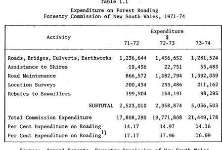
Forest roading affects all uses and users of forests, and expenditure on roading forms a significant part of overall expenditure by Australian Forest Services. Table 1.1 indicates, for example, the magnitude of the expenditure on roading by the Forestry Commission of New South Wales. The expenditures do not include professional salaries and expenses of officers involved in roading activities. Adding an allowance of 20% for overheads, to the roading costs shown in Table 1.1,
[image:11.537.42.503.50.717.2]Table 1.1
Expenditure on Forest Roading
Forestry Commission of New South Wales, 1971-74
Activity
71-72
Expenditure $
72-73 73-74
Roads, Bridges, Culverts , Earthworks 1,236,644 1,456,652 1,281,524
Assistance to Shires 19,456 22,751 53,483
Road Maintenance 866,572 1,082,794 1,392,039
Location Surveys 200,434 233,486 211,162
Rebates to Sawmillers 199,904 154,191 98,295
SUBTOTAL 2,523,010 2,958,874 3,036,503 Total Commission Expenditure 17,808,290 19,771,808 21,449,178 Per Cent Expenditure on Roading 14.17 14.97 14.16 Per Cent Expenditure on Roading"^ 17.17 17.96 16.99
[image:11.537.48.498.418.722.2]indicates that approximately 17% of total annual expenditure of the Forestry Commission of New South Wales goes towards forest roading.
The different costing and accounting procedures used by other State Forest Services makes comparison between the Services difficult. The direct costs for New South Wales, Queensland and Victoria are set out in Appendices 1.1, 1.2 and 1.3 respectively. In Queensland about
12% of Forest Service expenditure is directed toward roading and in Victoria about 9%. These percentages make no allowance for overheads.
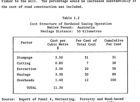
The relative costs of different forest operations are very variable, but the practical and economic significance of road haulage is indicated by Table 1.2, which illustrates the cost structure of a hard wood sawlog operation based on a native forest in Australia. In this operation, road haulage accounts for 30% of the cost of delivering timber to the mill. The percentage would be increased substantially if the cost of road construction was included.
Table 1.2
Cost Structure of Hardwood Sawlog Operation Native Forest:
Haulage Distance:
Australia 50 Kilometres
Factor Cost per
Cubic Metre $
Per Cent of Total Cost
Cumulative Per Cent
Stumpage 3.50 31 31
Cutting 0.80 7 38
Extraction 2.30 20 58
Haulage 3.30 30 88
Overheads 1.40 12 100
TOTAL 11.30
Source: Report of Panel 4, Harvesting. Forestry and Wood-based Industries Development Conference. Canberra, 1974.
[image:12.537.50.498.336.662.2]is usually recognized in providing funds for road construction and maintenance. Nevertheless, forest roading affects forest values other than those directly related to wood production, for example water resource, landscape, recreational and conservation.
While some of these values are causing emerging pressures on road systems that were not designed in relation to such values, the consequent pressures on the Forest Services and their resources have not produced responses from the State Treasuries, which would cover the cost involved in modifying current practices tied closely to the economics of the production of wood and other forest products. Nevertheless the widespread concern for the environment necessitates reorientation of the economic analyses and the traditional engineering approach to forest road system design.
In the United States, it has been claimed that the planning of a truly optimum forest road system is not possible at this time,
primarily because the data necessary for such an analysis is either inadequately defined or non-existent. Gardner [1971] suggests it is appropriate to use whatever rational means are available to evaluate protection of the environment.
In relation to the economic efficiency of the forest products industry, the effectiveness of road system design can be judged by hauling and travelling costs associated with the roads. It is the geometric characteristics, that is grade, vertical and horizontal
curvature, length of straight between curves, width, and sight distance which primarily determine haulage efficiency for a particular unit. For example, if roading is poorly designed and constructed, long haul times and queuing delays can result, truck loads may be reduced and wear and tear on trucks can increase very dramatically.
1.2 THE CLASSIFICATION AND DESIGN STANDARDS OF FOREST ROADS
The standards of construction of forest roads are usually specified in relation to a functional classification. Geometric
are difficulties associated with this for forest roads. The design speed parameters are determined by the reaction of cars and are not therefore a good indication of the speed at which heavily laden or empty trucks can travel the segment of the road [Armstrong, 1972].
The system of classification used by the Forestry Commission of New South Wales is one example of a number of systems. The function and standard of the road are used to describe a road as part of an overall roading system.
In terms of function, the roads are classified as: 1. Primary Access;
2. Secondary Access; 3. Feeder;
4. Link; 5. Track.
The standards are specified in terms of road width and design speed criteria, for four classes of road.
Class A: Two-lane all-weather road with a minimum pavement width of 5.5 metres, formation width 7.3 metres and meeting the requirements of at least 50 kph design speed.
Class’ B: All-weather road with a minimum pavement width of 3.7 metres, formation width 5.5 metres, and meeting the requirements of at least 30 kph design speed.
Class C: Single lane, substantially all-weather road, with a minimum pavement width of 3 metres, formation width 4.2 metres, with passing places, and meeting the requirements of at least 20 kph design speed.
Class D: Roads or tracks capable of use by conventional vehicles under dry or good conditions only and/or which do not meet the minimum 20 kph design speed criteria.
The geometric parameters for various design speeds are given in Table 1.3.
Table 1.3
Design Speed Criteria for Forest Roads Forestry Commission of New South Wales
Geometrical Parameters
100
Nominal Design Speed kph
80 60 50 30 20
Alignment
Minimum Radius
460 200 80 /;n 7 n 1 c
Curve (metres) D U 1 J
Minimum Length of
Straights (metres) 80 60 40 20 20 20
Grade (Per Cent)
Sustained Maximum : 4% 6% 6% 7% 8% 10%
Permissible Grade ^ : 6% 8% 8% 8% 10% 12*$%
(700) (500) (600) (300) (500) 12*$% (150)
^ Figures in brackets show the lengths in metres for which the permissible grade is allowed.
simple scheme to classify existing roads. It takes into account the main factors affecting speed (surface, grade, curves and width) and provides a uniform way of classifying existing roads by standard. Details of this system are shown in Appendix 1.4.
The approach to road classification by the Forestry Commission of New South Wales is typical of that adopted by many Forest Services and companies. Matthews [1942] outlines a system used by a large private firm in the United States, and Forbes [1961] describes the approach adopted by the United States Forest Service.
The determination of the standard of construction of roads, and the determination of the classification of roads, should be
1.3 FOREST ROADING PLANS
A forest roading plan sets out the optimal access for a forest or group of forests in relation to the projected management and harvesting operations. The preparation of the roading plan is one of the basic requirements for well planned management policies, and can avoid the piecemeal or ad hoc approach that seems to have been a characteristic of some forest roading programmes.
Theoretical techniques, described by Matthews (1942), Mandt (1973), Kirby (1973) and others are helpful in the preparation of a roading plan and can be used as guides for optimal planning but, as is stressed by Adamovich (1974), the preparation of a roading plan will always entail elements of both intuition and analysis based on practical experience and theoretical knowledge. The whole forest, its topography, physiography, anticipated major production zones and all other public and official uses should be considered in designing the layout of the road access
system.
The enactment of environmental protection legislation in some countries has forced reviews of the standards and construction practices associated with forest roads. Whereas there have been tendencies to
provide improved engineering standards to enable higher safe traffic speeds, there is now a tendency to lower some standards to lessen the environ
mental impact of roads by, for example, reducing the volume of earthworks. In responding to a requirement to reduce the environmental impact of roads by reducing standards of construction, a consequence would be increased haulage costs for wood but there is very little recent inform ation relating road standards to truck performance.
providing basic data that would enable improved selection of optimal standards for haulage roads in particular forests.
1.4 THE STUDY APPROACH
Over the past twenty years there has been a significant increase in the power of trucks used for log hauling. On the other hand the axle loads permitted on trucks has remained static in most States and thus it seemed that there may have been an increase in power relative to the loads hauled and consequently speeds maintained by trucks. It was concluded therefore that a review of maximum road gradients specified for forest roads based on quantitative measurements of actual log truck speeds on roads would make an effective and useful contribution to the general problem of optimizing forest road standards.
The speed of trucks on long adverse grades would obviously be related inter alia, to the load on the truck, and the load also has a considerable influence on the economics of haulage. It was decided therefore to link the investigation of actual log truck speeds on
particular gradients with a study of the variability of the loads hauled by log trucks.
The transport of logs from the plantations of the Australian Capital Territory was particularly suited to the study. Weighbridge data were available and the trucks hauled within the Australian Capital Territory and also to New South Wales, where much lower loads are
permitted, and a relatively large variation in loads hauled by trucks of the same type could be measured.
obtain the load carried by the truck when its speed was measured by reference to weighbridge dockets.
CHAPTER TWO
DATA COLLECTION AND PROCESSING
2.1 TRUCK LOADS
Wood from the plantations in the Australian Capital Territory is sold primarily by using a system which sets an estimated stumpage rate for the particular compartment (or group of compartments) prior to the commencement of the logging operations. At the completion of the logging on each area, an adjustment of the estimated stumpage is calculated. The adjustment is based on volume measurements of sample loads measured throughout the operation. All loads are weighed, and the volume measurements of the sample loads enable conversion of the total tonnage to a volume and log size class distribution for that area.
The weighbridge dockets record information from which the variability of the loads, within and between truck types hauling from the plantations, can be calculated. Speed readings on particular trucks could be matched with the load data recorded by the weighbridges.
Two weighbridges are in use, a public one at Kingston, and one operated by the A.C.T. Forests Branch at the mill of Integrated Forest Products Pty. Ltd.
The following information is recorded on a numbered docket at the Kingston weighbridge for each load of wood:
Truck registration Gross weight
Tare weight
Nett weight
Date
Origin of timber (for example Pierce's Creek)
Compartment number
Product destination.
The information on the dockets from the Kingston weighbridge
was transcribed in chronological order on computer coding forms. The
time when the load was weighed was obtained from the information on
diary sheets kept by a Forest Branch employee stationed at the weigh
bridge.
The dockets at the weighbridge at Integrated Forest Products
are automatically stamped with:
Date
Time of arrival
Gross weight
Time out
Tare weight
Market (usually Integrated Forest Products).
The operator at the weighbridge records:
Truck and trailer numbers
Nett weight
Forest of origin
Compartment
Product type
Sample loads.
The A.C.T. Forests Branch imposes a limit of forty eight
tonnes gross vehicle weight on all loads. If a load is substantially
above this, the driver is required to unload some of the wood to bring
the gross weight below the allowable limit. The broken down load is
then measured as two loads. Such occurrences are obvious on the weigh
bridge dockets. In coding the data from the weighbridge at Integrated
Forest Products on computer coding forms, a symbol was used to indicate
that two loads may in fact represent one load hauled along the road.
from 23rd June 1975 until the 30th August 1975. The coded data were punched on to computer cards for subsequent calculations. A computer program was prepared to check that the data was correctly transcribed by
scanning the information for irregularities and errors. The listing for this program is shown in Appendix 2.1.
2.2 TRUCK SPEEDS
2.2.1 Sites for Measurement of Speed
Selection of Sites
The basic requirement of the sites was a range of grades over which log trucks would be travelling at a frequency that would enable information to be gathered at a reasonable rate. The radar meter was on loan for about three months and a full day in the field for only one or two truck loads could not be justified.
Each section of road selected as a study site had to be of sufficient length for the effect of grade on speed to be substantial. Preliminary measurements had indicated that this should preferably be a straight, of at least 150 metres. In reconnaissance surveys for
possible sites, this was an important parameter which limited the number of sites available.
The A.C.T. Forests Branch provided information on the current and proposed cutting programme to assist in the selection of roads where log truck traffic could be expected. Unfortunately, wet weather during the field measurement phase of the study disrupted the cutting plan to some extent. The special arrangements associated with salvaging wind-thrown trees also added to the disruption of the cutting plan. For
%
Tlie selection of long, straight and continuous grades on forest roads in the A.C.T. proved virtually impossible, as in general these roads are of low standard. This, together with low numbers of log trucks passing along them because of the dispersed nature of the
operations, made it more effective to select sites on the public roads leading to the forests. Four sites were selected along the Mt. McDonald Road between the Uriarra Forestry Settlement and the Cotter Reserve. Virtually all the wood hauled from Uriarra Forest must go over these sites.
Location of Sites
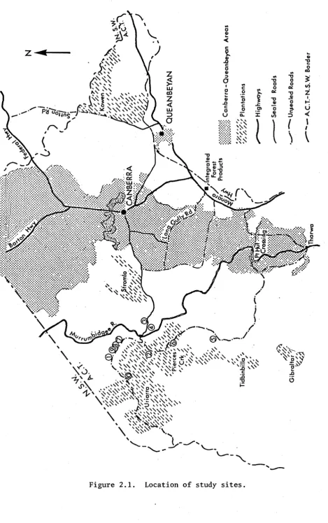
The general location of the sites was as follows. Sites 1, 7, 8 and 9 were located on the Mt. McDonald Road. Sites 2 and 5 on the Laurel Camp Road, which is the access road to Pierce’s Creek Forest. Sites 3 and 4 were on the Cotter Road above the Cotter pumping station. These two sites provided long, continuous grades. Site 6 on the Paddy’s River Road was the steepest site chosen. Site 10 was on the Brindabella Road and like site 6 was downhill with the load. The location of the sites is shown in Figure 2.1.
Ground Surveys
The following information was required at each site: Grade
Pavement Width Length of Section Horizontal Curvature.
The survey information was obtained quite simply with an Abney level, Suunto compass and metric band or tape, but nevertheless required a number of days in the field. The procedure was to measure grade, distance, pavement width and bearing from each successive station to the next along the road. Notes were made on the surface type and any other
\ ® V "
v \ ,\\VX\ n'\.
•
rsOs^ ' < ^ ' i p c ^ ' v
''>'-'S$
V ' ' \ > V > -\^E' '2's'
vidvcr. s' s
.
•
\ ^ ' V W . V v
c 15
% ■ : -V s w i p
s>
b
\o «
\
N\
K N — t V N N
P P "
V.L-.
X
Figure 2.1. Location of study sites.
j
a
p
j
o
g
M
'
S
N
-T
D
[image:23.537.32.502.46.795.2]SE C T IO N 2
100 200
HORIZONTAL DISTANCE ( m e t r e s )
SECTION 1
HORIZONTAL DISTANCE ( m e t r e s )
4-25%
2 -10
[image:24.537.9.508.43.781.2]S
E
C
T
IO
N
REDUCED LEVEL ( m e t r e s )
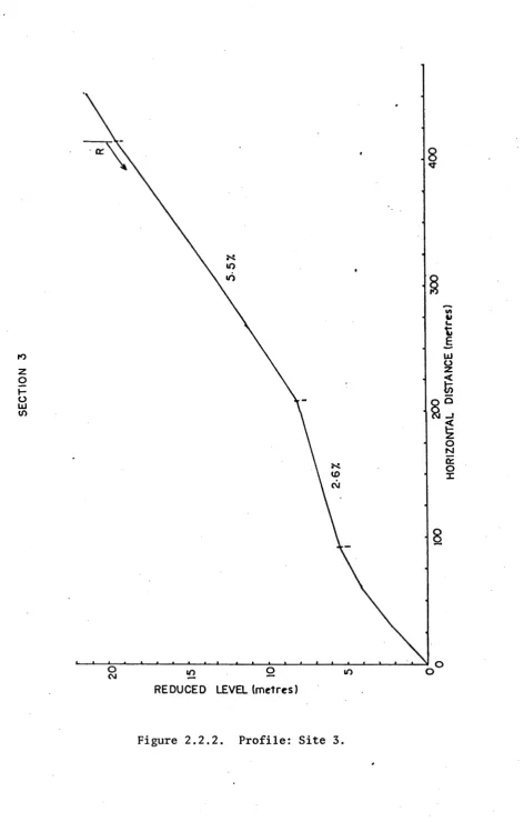
Figure 2.2.2. Profile: Site 3.
H
O
R
IZ
O
N
T
A
[image:25.537.45.518.60.801.2]16
6-06%
100
HORIZONTAL DISTANCE (m e tre s )
SECTION 4
7-05%
6-6 8%
6-98%
200
HORIZONTAL DISTANCE (m etres)
[image:26.537.24.486.60.657.2]R
E
D
U
C
E
D
L
E
V
E
L
(m
e
tr
e
s
)
SECTION 6
1007
.
100 2 0 0
[image:27.537.43.492.65.706.2]R
ED
UC
ED
L
E
V
E
L
(
m
e
tr
e
s
)
RE
DU
CE
D
LEVEL
(m
e
tr
e
s
)
SECTION 8
IOO
HORIZONTAL DISTANCE (metres)
SECTION 7
100 200
HORIZONTAL DISTANCE Im e tre s )
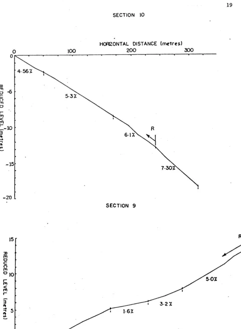
[image:28.537.48.502.63.798.2]SECTION 10
HORIZONTAL DISTANCE ( m e t r e s )
4 56 7.
SECTION 9
200
HORIZONTAL DISTANCE ( m e t r e s )
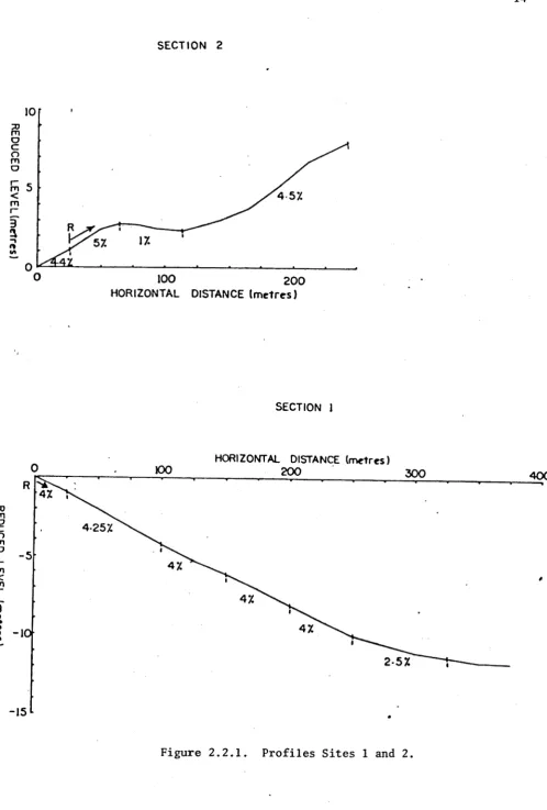
[image:29.537.18.499.30.685.2]The letter ' R* on these plans indicates the position of the radome and the direction in which it is pointing, the radome being the
signal transmitting and receiving aparatus.
Description of Sites
Site 1: Mt. McDonald Road
The radar was located at the top of the grade and about 450 metres from a T intersection with a road to Uriarra Forest Station. Approaching trucks negotiated several curves and an adverse grade, and then, approximately 500 metres away came down a short hill on to the flat near the intersection. The grades over the 400 metres
leading to the radar meter were then: 400 to 250 metres 250 to 100 metres 100 to 25 metres
25 to 0 metres
2.5% rise 4.0% rise 4.25% rise 4.00% rise
The 4% grade continued for a further 50 metres before levelling and entering a corner.
The average pavement width for the site was 5.6 metres and the surface was compacted gravel in reasonable condition.
Site 2: Laurel Camp Road
Leaving the radar in the direction of the beam there was a 5% rising grade for 40 metres, followed by a 1% fall for 50 metres and then ,4.5% rising for 90 metres. This was the extent of the radar beam’s line.
The grade continued rising at 4.5% into two curves beyond the limit of the meter.
This site did not prove very useful as far as grade effects were concerned as alignment and a narrow, rough pavement also caused reductions in speed.
Site 3: Cotter Road
The pavement of the Cotter Road had a bitumen surface.
The radar was at the top of a slope and loaded trucks climbed toward it. The grades going down from the radar were as follows:
0 to 107 metres 5.7% falling 107 to 207 metres 5.2% falling 207 to 323 metres 2.6% falling.
The grade then increased to 6% (falling) for 92 metres around a horizontal curve of 205 metres radius to the location of site 4.
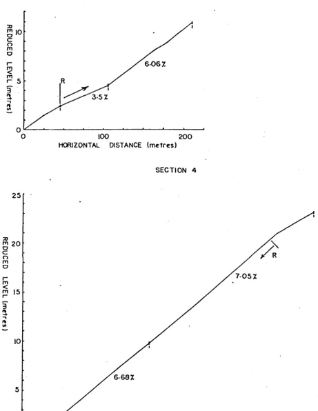
Site 4: Cotter Road
The radar was directed down the grade which was as follows for distances from the radar:
0 to 207 metres 7.1% falling 207 to 271 metres 6.6% falling
These sections were followed by a horizontal curve of approximately 190 metres radius and the road moved away from the direction of the radar beam. The grades were then 7% (falling) for 44 metres and 5% (falling) for another 50 metres.
Site 5: Laurel Camp Road
This site had to be abandoned. It was not used by log trucks at the time of field measurements because of wet weather. However, speed measurements for several other vehicles were recorded.
The radar was at the bottom of a slope and pointing up it. The grades for distances from the meter were as follows:
0 to 60 metres 3.5% (rising) 60 to 164 metres 6.0% (rising).
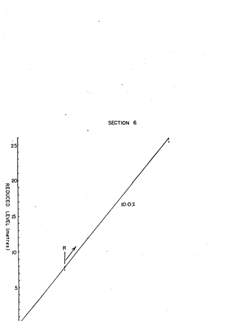
S i t e 6 : Paddy*s R i v e r Road
The P a d d y 's R i v e r Road i s a b itu m e n s u r f a c e d , t w o - l a n e r o a d and a t
t h i s s i t e t h e r e was a c o n s t a n t 10% f a l l i n g g r a d e f o r 180 m e t r e s a l o n g a
s t r a i g h t t o t h e r a d a r . The s t r a i g h t c o n t i n u e d f o r a n o t h e r 80 m e t r e s
p a s t t h e r a d a r b e f o r e e n t e r i n g a c u r v e .
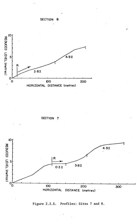
S i t e 7: Mt. McDonald Road
The r a d a r beam was aimed up t h e s l o p e and a s t h e m a j o r i t y o f t h e
t r u c k s t r a v e l l e d up t h e s l o p e t h e i r s p e e d s were m e asu re d as t h e y moved
away from t h e m e t e r .
R e f e r r i n g t o F i g u r e 2 . 2 . 5 , t h e r o a d was s t r a i g h t from t h e m e t e r ,
a t t h e 105 m e tr e mark t o a b o u t 250 m e t r e s . A h o r i z o n t a l c u r v e o f
a p p r o x i m a t e l y 55 m e t r e s r a d i u s p r e c e d e d t h e r a d a r m e te r p o s i t i o n . The
g e o m e try o f t h e g r a d e a t t h i s s i t e was r e l a t i v e l y co m p lex . The h o r i z o n t a l
c u r v e p r e c e d i n g t h e m e t e r was a t a r i s i n g g r a d e o f 4.6%. I n t h e s i g n a l
p a t h t h e r e w ere r i s i n g g r a d e s o f 0.25% f o r 40 m e t r e s , 3.8% f o r 60 m e t r e s
and t h e n 4.9% f o r 40 m e t r e s . The 3.8% and 4.9% g r a d e s w ere e q u i v a l e n t
t o 4.25% o v e r t h e 100 m e t r e s .
A verage p avem ent w i d t h was 6 m e t r e s w ith a g r a v e l s u r f a c e .
S i t e 8: Mt. McDonald Road
The r a d a r was aimed u p s l o p e a t t h i s s i t e , t h e g r a d e s b e i n g 2.8%
f o r 100 m e t r e s and t h e n 4.9% f o r 60 m e t r e s . The s t r a i g h t t h e n e n t e r e d
a 180 m e tr e r a d i u s c u r v e .
The a v e r a g e p av em en t w i d t h was 6 . 6 m e tr e s w i t h a g r a v e l s u r f a c e .
The s i t e was u p h i l l from s i t e 9 . A h o r i z o n t a l c u r v e o f 110 m e t r e
r a d i u s w i t h a g r a d e o f 5% s e p a r a t e d t h e two s i t e s .
S i t e 9 : Mt, McDonald Road
The r a d a r was a t t h e t o p o f t h e s l o p e on t h e 110 m e tr e r a d i u s
the radar w a s :
0 to 100 metres 5% (downhill) 100 to 160 metres 3.2% (downhill) 160 to 210 metres 1.6% (downhill).
A horizontal curve of 270 metre radius with a grade of 3.7% followed.
The average pavement width was 6.6 metres with a gravel surface.
Site 10: Brindabella Road
The radar was set up on a horizontal curve of 120 metres radius and above a 7.3% grade. Loaded log trucks moved down the grade. The grades moving away in the direction of the radar beam were as
follows:
0 to 60 metres 6.1% (downhill in direction of trucks) 100 to 180 metres 5.3% (downhill in direction of trucks). Beyond this straight was a grade of 4.6% around a horizontal curve of 200 metres radius.
The average pavement width was 5 metres with a gravel surface.
2.2.2 Speed Measurement
Equipment
A Traff-O-Matic, Model S-5, Radar Speed Meter and Graphic Recorder were borrowed from the National Capital Development Commission. This was the only radar meter available in Canberra with a Graphic Recorder.
The equipment measures the instantaneous speeds of moving vehicles and is a portable unit easily mounted on any vehicle with a 12 volt electrical system. It comprises four major components:
(i) Radio Frequency Head Assembly (Radome); (ii) Amplifier and Power Supply Assembly;
indicator); (iv) Graphic Recorder.
Details of the specifications of the Radar Speed Meter are given in the technical manual provided by the manufacturers.1^ The operating range of the unit was 0 to 160 kilometres per hour with a stated accuracy of plus or minus 3.2 kilometres per hour. The unit operates on the Doppler principle, that is on the change in the frequency when a wave is reflected from a moving target. The radome consisted of a radar transmitter and receiver and the meter detected the change in frequency in the reflected signal and converted it to the speed of the vehicle. The speed was indicated on the Indicator Assembly and Graphic Recorder.
A three position switch on the Amplifier and Power Supply Assembly provided for one of three ranges to be selected. The ranges were approximately 50, 100 and 150 metres with the radome one metre above the ground, and an unobstructed line of sight. In all the ranges, signals could be obtained for distances over twice the nominal range. The speed readings for the study were taken with the radome 1.5 metres
above the ground to gain a longer unobstructed view.
Field Set-up of Equipment
Preliminary testing of the equipment in the field and the suggested operational procedures in the manual led to a number of important requirements when setting up the equipment in the field.
The equipment had to be set up as far as possible off the road to avoid interference with the traffic flow, still keeping the angle between the path of the vehicle and the radar beam at less than ten degrees. This was to ensure that the error in the readings, due to the inclination of the radar beam to the line of travel, was less than 2%.
The amplifier and power supply assembly required at least five minutes to warm up before readings could be taken. After this warm-up period, a calibration check was carried out, using a calibration tuning fork supplied with the equipment. The vibrating tuning fork was held vertically 7 - 1 5 cm in front of the radome and the frequency
corresponded to an approaching speed of 64 kilometres per hour (40 mph).
Field Recording Procedures
Two cams were fitted to the graphic recorder enabling a choice of two chart drive speeds, namely 15 cm per hour or 15 cm per minute. After initial test runs it was considered that a chart drive of 15 cm per hour produced charts which enabled interpretation only in terms of maximum speed. The faster drive speed was therefore used and this produced a profile 'from which speeds at 2.5 second intervals could be obtained.
Examples of charts obtained with each of the two drive speeds are shown in Appendix 2.2.
A record was kept of every vehicle for which speed measure ments were taken but only the data for log trucks was processed. The following information was recorded on the chart of the meter:
Time
Vehicle Make and Type (for example, Volvo G88 Semitrailer) Registration Number of Prime Mover (and trailer if applicable) Loaded or Empty
Direction of Travel with respect to Grade (that is up or down). Notes were also made of any features regarding the performance of the truck during its passage through the measuring site which might assist subsequent interpretation of the performance of the vehicle and driver.
The following information was noted for vehicles other than log trucks:
Time
Vehicle Make and Type
Direction of Travel with respect to Grade (that is up or down) . The nature of the load usually carried was also noted for trucks and whether the truck was loaded.
It was convenient to record some of this information directly on the charts, along with the vehicle make and type. On some occasions it was possible to note on the charts the time, and such other events as gear changes and interference from other vehicles.
Problems Associated with Field Measurements
It was expected that the radar meter would attract attention and possibly cause normal performance to be modified. It was very desirable for example to avoid drivers slowing down to enable a closer
look at the instrument set-up. In two cases, trucks actually stopped at the set-up and the driver enquired what was being measured.
An endeavour was made to contact all log truck drivers and explain to them the nature of the measurements, request that they
disregard the meter as far as possible, and assure them that it was not a radar speed trap. The efforts made seemed to be fairly successful and most log truck drivers were aware of the position of the meter and many of them subsequently saw the charts. Nevertheless, it was not always possible to make contact with drivers before taking measurements and on several occasions trucks obviously slowed down. In these cases the data was discarded, somewhat reluctantly as sometimes only six trucks would be measured in one day. On one occasion, the driver of an unloaded vehicle was moving at an almost "breakneck” speed and it was assumed that this was a deliberate response to his knowledge of the location of the meter and, although the reading was discarded for the purposes of this study, a speed of 120 kilometers per hour for an unloaded log truck on a gravel road is worth noting.
radome on long steep slopes.
It is common with microwave multipath transmission for signal cancellation to occur when a vehicle comes within range. The indicator needles swing up to the speed reading and then drop momentarily towards zero, one or more times. This phenomena sometimes made interpretation of the charts more difficult, and an example is shown in Appendix 2.3.
There were also occasional problems with the ink flow in the pen of the chart recorder, particularly on cold mornings when the temperature was about zero, and some recordings were lost because the ink did not flow.
The needle on the graphical recorder sometimes rose slowly and gave speeds which were less than those shown on the indicator assembly. This was often pronounced in the first few seconds of the signal from a distant, fast-moving vehicle approaching the meter. When a vehicle passed the radome the signal often showed a kick up but this was easily distinguishable from the rest of the recording and probably due to the angle between the beam and the vehicle path exceeding ten degrees.
Intermittent signals were often obtained when log trucks were travelling at less than 10 kilometers per hour and this was contrary to the claims of the manufacturers that continuous measurements could be obtained down to zero speed.
A most frustrating problem was interference to, or masking of, the main signal by vehicles travelling in the opposite direction or overtaking the slower moving log trucks. At times it seemed that with only three vehicles per hour passing the meter two would always pass at the same time.
Location of Vehicles on Road Profiles at Time of Speed Measurement
The actual position of the radome was noted on the survey profiles and recorded with reasonable accuracy on the graphs produced by the Chart Recorder for each vehicle passage. This information was
necessary to fix recorded vehicle positions with respect to the position of the vehicle on the ground.
The position of the radome on the chart was used as a base point and the fraction of time to the next 2.5 second interval on the graph paper was recorded, on data coding forms, as the first time
interval. The speed at the radome and at 2.5 second intervals was also recorded on the coding forms. This information was subsequently
computed to determine the speed at various points along the road at the site.
The information on whether the truck was approaching or leaving the radar provided the record as to whether the truck was ascending or descending the grade, for the radar was always located at the same position at each site. Table 2.1 summarizes the radar position and the usual direction of travel of loaded trucks but it was necessary to check each trip as some trucks passed empty in the loaded direction.
The data on the coding forms was punched on to computer cards and a program written to check for any errors or
irregularities.-2.3 TRUCK CAPACITIES
The following data was required for each truck: Configuration
Number of axles
Tabletop, semitrailer, jinker, etc. Power rating
[image:38.537.42.479.352.749.2]Table 2.1
Radar Positions and Direction of Travel
Site Radar Usual Direction
Number Position-^) of Loaded Trucks^)
1 Top Uphill towards
2 Bottom Downhill towards
3 Top Uphill towards
4 Top Uphill towards
5 Bottom Downhill towards
6 Bottom Downhill towards
7 Bottom Uphill away
8 Bottom Uphill away
9 Top Uphill towards
10 Bottom Downhill towards
^ With respect to grade. 21
With respect to radar.
Data Collection
Information on the configuration of the trucks was collected in the field concurrently with other data collection and also from officers and employees of the A.C.T. Forests Branch.
Data on power ratings was obtained from the truck drivers at the weighbridges through the co-operation and assistance of employees of the Forests Branch. Additional information on Volvo trucks was obtained from discussions with the Volvo (Australia) dealer in Queanbeyan.
In answer to a written request the Department of Main Roads, New South Wales, provided information on the regulations in that State regarding maximum axle loads and loaded weights. This information is in Appendix 2.4 and enables permissible loads to be assessed.
tonnes.
Although apparently straightforward, a number of difficulties were encountered in collating the information on configurations and power ratings.
The configurations of trucks can be changed and the
manufacturer's information had to be checked. For example, a Leyland truck had the chassis of its prime mover lengthened and a longer tray added. The truck had previously towed a trailer and carried short logs on the truck and the trailer.
The collection of individual truck power ratings presented some difficulties. Manufacturers express the power rating in two ways. The first is an indication of the power produced by the motor (SAE), the second the power delivered to the drive shaft (DIN). Volvo, for example, use the second method.
Power varies with the state of repair and tuning of the motor but there was no practicable way to account for this in this study and the Tated values nominated by the manufacturers have been used.
Several of the trucks hauling the logs had modified motors fitted to the trucks or other modifications such as different injectors. In such cases, reliance had to be placed on the information supplied by the driver and wherever possible this was discussed personally. In the cases where this was not possible, information collected at the weigh bridge from the driver was accepted after checking against manufacturers specifications.
CHAPTER THREE
ANALYSIS OF LOG TRUCK SPEEDS IN THE A.C.T.
PART A : INTRODUCTION
3.1 EXAMINATION OF RADAR DATA
Introduction
As previously indicated in Chapter Two, the analogue charts obtained from the radar meter gave information on the velocity of the vehicles with respect to time. While this would be adequate for many applications of the radar meter, including speed checks, it was
necessary in this study to relate the speed of the vehicle to the position on the road.
The first step was to plot the velocity of each truck with respect to distance from the meter, so that the velocity at any point on the road profile could be determined.
In the preliminary analysis of the data to develop and check the methods, information from selected sites and trucks was computed and plotted manually. It seemed that patterns could be determined in the velocity of trucks at certain points on the road profiles and it was then decided to prepare all the graphs for the ten sites. The
The method developed was to obtain truck velocity at 2.5 second intervals from the analogue charts recorded by the radar meter and code this information for computation by a computer. The data were computer sorted in chronological order according to site, truck, and direction of travel.
The distance travelled by the truck in each time interval was calculated assuming the mean velocity for the time interval. Beginning at time zero, when the truck passed the radar meter, the speed at the Various distances from the meter was calculated by accumulating the distance travelled in successive time intervals.
The road survey profiles for each site were then superimposed on the graphs so that the speeds could be co-ordinated with various road geometry factors. This could be done with an accuracy of plus or minus ten metres, as the radar position had been marked on the site surveys. The main source of inaccuracy in relating the speed to the ground survey was in determining, on the field charts, when the truck actually reached or passed the radar meter. As noted previously, the speed and time at the radar meter constituted the datum for the computation of the speed-distance graphs.
There were several gradients at each site, and the speed at each change of grade was extracted and then also speeds at intervals of 50 metres. In some cases the charts had irregularities near the 50 metre
intervals (e.g. from gear changes). Speeds were then taken at 25 metre intervals to try to get a more accurate estimate of the speed with respect to distance.
In addition to plotting the information for visual study, the speed-distance information was tabulated as computer print-out along with the vehicle identification, direction of travel and gross weight. Examples of the print-out are shown in Appendix 3.2.
The maximum speed and the reduction from this over particular uphill gradients were recorded and the graphs examined to select those which could be used to formulate models to predict the speeds of log trucks on various grades in terms of the parameters measured in this study.
The ratio, power to weight, was adopted for the testing of model.formul ations. Power was expressed in watts and weight in kilograms. This ratio was used by Byrne
et al.
[1960] for travel time predictions on various grades.The relationships which might exist between speed (used as the dependent variable) and power to weight and grade (as the independent variables) were examined using manual techniques; to try and ascertain the form that relationships derived from the data might take and to make preliminary comparisons with theoretical relationships such as power related to velocity for a given load. The theoretical relationships are outlined by Byrne
et al.
[1960] and Armstrong [1972].It became clear that computerized techniques would have to be adopted to best test and validate models and the statistical techniques available were therefore reviewed in relation to the analysis of this data.
PART B : ANALYTICAL PROCEDURES
3.2 STATISTICAL CONSIDERATIONS
In many areas of research where controlled experiments are not practicable, the techniques of multiple regression analysis are commonly used to quantify the effects of different X-variables on some response Y. The determination of the relationship of a dependent variable Y, with a number of independent variables Y^ is commonly required in forestry research, and is the problem encountered in this study.
Specific reference to the use of linear regression analysis techniques in forestry research is made in Freese [1964], Snedecor and Cochran [1967], Draper and Smith [1966] and Leech [1973]. Linear analysis refers to linearity in the parameters of the type
Y = + + $2^2 ••• ^p^p + ^ *
X^, X ^ j X ^ . ^ o X ^ ; 3q ,^^ e t c . r e p r e s e n t c o e f f i c i e n t s (w hich a r e c o n s t a n t s )
and E i s an e r r o r t e r m .
N o n - l i n e a r r e g r e s s i o n a n a l y s i s r e f e r s t o f u n c t i o n s which a r e n o n
l i n e a r i n t h e p a r a m e t e r s , f o r exam ple
Y =
91
(VV - e-Vl ♦ e.
8 1 - 02 L J
N o n - l i n e a r r e g r e s s i o n a n a l y s e s a r e l e s s commonly u s e d a s t h e y he e n o t
b e e n i n t e g r a t e d i n t o a t h e o r y o f t h e same d e g r e e o f g e n e r a l i t y a s t h a t
w hich a p p l i e s t o t h e l i n e a r c a s e ( S n e d e c o r and C o c h ra n , 1967; F r e e s e ,
1 9 6 4 ) .
I n t h i s s t u d y , an a p p ro a c h u s i n g l i n e a r r e g r e s s i o n a n a l y s i s was
a d o p t e d f o r t h r e e main r e a s o n s :
1. A lth o u g h c o n s i d e r a b l e ti m e had b e e n s p e n t i n t h e f i e l d , t h e
amount and r a n g e o f t h e d a t a o b t a i n e d was l i m i t e d b y b o th t h e
t i m e a v a i l a b l e f o r c o l l e c t i o n and t h e s i t e s and t r u c k s a v a i l a b l e
f o r o b s e r v a t i o n . More r e f i n e d a n a l y s e s would n o t t h e r e f o r e
im p ro v e t h e r e s u l t s o b t a i n e d .
2. The form o f t h e t r u e model was n o t a v a i l a b l e b y s im p le t h e o r e t i c a l
c o n s i d e r a t i o n s and t h e r e f o r e t h e r e was no i n d i c a t i o n t h a t no n
l i n e a r form s would a c t u a l l y be r e q u i r e d .
3 . P a c k a g e co m p u te r p ro g ram s w hich c o u l d b e i n d e p e n d e n t l y h a n d le d
and i n t e r p r e t e d were r e a d i l y a v a i l a b l e f o r l i n e a r r e g r e s s i o n ,
and i n p a r t i c u l a r , t h e REX p ro g ram (G ro se n b a u g h , 1 9 6 7 ).
A number o f t h e more g e n e r a l p r o b le m s i n m u l t i p l e l i n e a r r e g r e s s i o n
a n a l y s i s w ere a p p l i c a b l e t o t h i s s t u d y . In t h i s t y p e o f a n a l y s i s ,
t h e r e s p o n s e o f t h e d e p e n d e n t v a r i a b l e (Y) i s gauged a g a i n s t t h e
e f f e c t s o f d i f f e r e n t in d e p e n d e n t v a r i a b l e s (X’ s ) . I t was n o t p o s s i b l e
i n t h e t y p e o f m easu re m en ts made i n t h i s s t u d y t o e n s u r e t h a t X v a l u e s
o t h e r t h a n p o w e r , w e ig h t and g r a d e were n o t r e l a t e d t o Y ( s p e e d ) i n t h e
s am p led p o p u l a t i o n . These o t h e r v a l u e s a r e d i s c u s s e d i n S e c t i o n 3 . 4 . 1 .
I f one o r more o t h e r r e l a t e d X v a l u e s e x i s t , t h e e s t i m a t e d
v a l u e o f t h e c o e f f i c i e n t s o f X i n t h e computed r e g r e s s i o n from t h e
sa m p le would n o t b e u n b i a s s e d e s t i m a t e s o f t h e p o p u l a t i o n ’ s c o e f f i c i e n t s
coefficient may then be over- or underestimated. The amount of bias in the coefficients depends on the variables that have not been measured and it is difficult to make a judgement on the magnitude of the bias.
However, where the primary objective of the analysis is to provide an accurate prediction of Y rather than separate the effects of the various independent variables, the bias may be of assistance. If the unknown variables were good predictors of Y and have stable
relationships with particular X variables, then the prediction of Y would be improved as the coefficients of the independent variables incorporate the effects of the unknowns.
The REX program [op. cit. , p.34] uses a least squares type of linear regression analysis. Four major assumptions are made in this type of analysis. The assumptions concern the residuals (or errors) present. Therefore, after fitting a curve to the data to form a
mathematical model, it is necessary to ascertain whether the residuals exhibit tendencies which confirm, or at least do not deny, the
assumptions. The assumptions are: 1. Homogeneity of the variance; 2. There is no measurement error;
3. There is no serial correlation between residuals; 4. The residuals follow a normal distribution.
1. Homogeneity of the Variance
The fitting of an unweighted regression assumes that the
dependent variable has the same degree of variability (variance) for all levels of the independent variables [Freese, 1967]. That is to say that the sample data is from a population for which the variance is
homogeneous and the variance of the residual term of the regression is constant over the range of the regression data. If the variance was heterogeneous, then the estimates of coefficients in the regression would be less precise than if homogeneous.
More precise estimates of the coefficients can be obtained in cases where the variance is heterogeneous by using weighted regression fitting procedures (Freese, 1964; Snedecor and Cochran, 1967). This may eliminate or reduce heterogeneity to acceptable levels. If weight ing is not used in such cases, the estimates would not have minimum variance as this would be obtained from the correct weighted least squares analysis.
Three commonly used tests for homogeneity of variance are discussed by Leech (1973). Leech favours Bartlett's test (Bartlett,
1937), as it allows for differing numbers of observations. The test procedure is also outlined by Freese (1964) and this test was adopted in analysing the data in these investigations. Snedecor and Cochran
(1967) urge caution when using the test as it is sensitive to non normality in the data, particularly kurtosis, and with long tailed
distributions (positive kurtosis) can give erroneous verdicts of hetero geneity.
The procedure in testing for homogeneity of variance in this study was as follows. If heterogeneous trends were evident, a weighting fac tor was developed which was then used in the development of the
regression models. When a model had been selected it was further tested using Bartlett's technique. The data was arranged in order according to the dependent variable and then divided into approximately equal groups. The variance within each group was then calculated and a value for chi-squared obtained. This was tested against the "Accumulative Distribut ion of Chi-square" as given in Table 4 of Freese (1967) for the desired probability level. The assumption of homogeneity was rejected if the calculated value was greater than that in the Table. If rejected, the weighting factor was redetermined and again applied to the data. The revised model was then tested again and the "cut and trial" proced ure continued until Bartlett's test did not reject the assumption of homogeneity.
2. Measurement Error