Inferring diffusion in single live cells at the single-molecule level

This is a repository copy of Inferring diffusion in single live cells at the single-molecule level.

White Rose Research Online URL for this paper: http://eprints.whiterose.ac.uk/84954/

Version: Accepted Version Article:

Robson, Alex, Burrage, Kevin and Leake, Mark C orcid.org/0000-0002-1715-1249 (2013) Inferring diffusion in single live cells at the single-molecule level. Philosophical

Transactions Of The Royal Society Of London Series B - Biological Sciences. 20120029. pp. 1-14. ISSN 1471-2970

https://doi.org/10.1098/rstb.2012.0029

[email protected] https://eprints.whiterose.ac.uk/

Reuse

Items deposited in White Rose Research Online are protected by copyright, with all rights reserved unless indicated otherwise. They may be downloaded and/or printed for private study, or other acts as permitted by national copyright laws. The publisher or other rights holders may allow further reproduction and re-use of the full text version. This is indicated by the licence information on the White Rose Research Online record for the item.

Takedown

If you consider content in White Rose Research Online to be in breach of UK law, please notify us by

Philosophical Transactions B.

Inferring diffusion in single live cells at the single

molecule level

Alex Robson1_{, Kevin Burrage,} 2, 3 _{and Mark C. Leake}1, 4,*

1_{Clarendon Laboratory, Dept of Physics, Parks Road, Oxford University, Oxford OX1}

3PU, UK, 2 _{Department of Computer Science, Wolfson Building, Parks Road, Oxford}

OX1 3QD, UK, 3_{Mathematics Department, QUT, Brisbane QLD 4001, Australia;} 4_{Dept of}

Biochemistry South Parks Road Oxford, OX1 3QU, UK.

*_{Correspondence: [email protected]}

Received Philtrans B 20 July, 2012. Accepted Philtrans B 20 August 2012.

Contributed original research article to theme issue of PhiltransB “Single molecule

ABSTRACT

The movement of molecules inside living cells is a fundamental feature of biological

processes. The ability to both observe and analyse the details of molecular diffusion in

vivo at the single molecule and single cell level can add significant insight into

understanding molecular architectures of diffusing molecules and the nanoscale environment in which the molecules diffuse. The tool of choice for monitoring dynamic molecular localization in live cells is fluorescence microscopy, especially so combining total internal reflection fluorescence (TIRF) with the use of fluorescent protein (FP) reporters in offering exceptional imaging contrast for dynamic processes in the cell membrane under relatively physiological conditions compared to competing single molecule techniques. There exist several different complex modes of diffusion, and discriminating these from each other is challenging at the molecular level due to

underlying stochastic behaviour. Analysis is traditionally performed using mean

square displacements of tracked particles, however, this generally requires more

data points than is typical for single FP tracks due to photophysical instability. Presented here is a novel approach allowing robust Ba yesian r anking of d iffusion

processes (BARD) to discriminate multiple complex modes probabilistically. It is a computational approach which biologists can use to understand single molecule features in live cells.

Keywords/phrases: Diffusion, confinement, fluorescent proteins, in vivo imaging,

single particle tracking, membrane heterogeneity

1. INTRODUCTION

Biological processes in the cell membrane are hard to replicate in artificial bio-mimetic membranes in vitro as the native protein-lipid architectures and dynamics in the

underlying membrane sub-structure that maintains the observed heterogeneity. Several observations have led to this hypothesis; on a macroscopic length scale of several hundred nanometres, the diffusion coefficient of proteins are one to two orders of magnitude lower than those observed in artificial membranes [4-9], also the observation that membrane proteins have dramatic drops in diffusion rates upon oligomerization or aggregation [4, 10, 11], incommensurate with Saffman-Delbrück modelling [12, 13] which represents the standard analytical method for characterizing the frictional drag of protein molecules in lipid bilayers. Non-specific interactions are also attributed to membrane heterogeneity; for example, simple lipid bilayers protein-lipid and lipid-lipid interactions can cause proteins to partition into self-associating clusters [14], creating protein-rich or poor regions in cells. Also, there is some evidence for regions of lipid micro- and nanoscale structure identified in some eukaryotic membranes commonly referred to as lipid “rafts”, which often appear to be consistent with mobile regions of phase-separated membrane that exist in an ordered, dense liquid phase surrounded by a more fluidic phase [15, 16]. These may be of functional advantage to signalling systems as well as being implicated in protein partitioning.

What is apparent is that there exists significant heterogeneity in local membrane architecture for a range of important biological functions. A key method for investigating the complex environment of the cell membrane is to monitor the fine details of diffusion of single molecules and complexes in native membranes. A tool of choice is fluorescence microscopy. This offers relatively minimal perturbation to native physiology whilst presenting an exceptional imaging contrast at single-molecule sensitivity levels that can allow the movement of individual fluorophore-tagged molecules, such as proteins and lipids, to be tracked with nanoscale precision [17-19].

membrane. SPT of fluorescently-labelled particles in the membrane offers significant advantages in using a much smaller probe on the nanometre scale. This was first applied using organic dye labelling [21, 22], but the recent use of genomically-encoded fluorescent protein (FP) reporters, such as green fluorescent protein (GFP) and its different coloured variants, has enabled many SPT studies to be performed on living cells with exceptional tagging specificity for the protein under investigation [23].

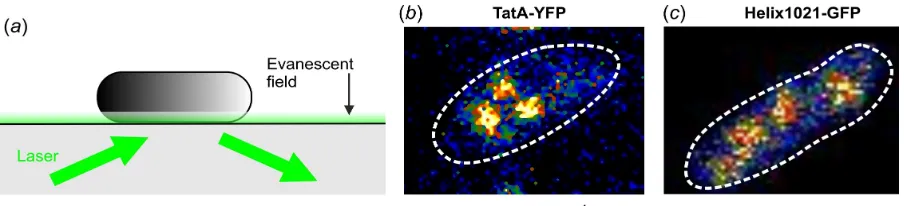
The most robust fluorescence imaging method for probing molecular level localization in the cell membrane is TIRF microscopy (see [24] for a discussion). This uses typically laser excitation at a highly oblique angle of incidence to generate an evanescent excitation field in the water-based environment of the sample - this can be thought of as an “optical slice” of ~100 nm thickness on the surface of the glass microscope slide/coverslip on which a cell sample is mounted. This results in significant excitation of fluorescently-labelled molecules in the cell membrane in the vicinity of the slide/coverslip surface. There is minimal excitation of components beyond this, either in the cell or from background fluorescence in the physiological buffer, therefore the signal-to-noise ratio for imaging membrane components is increased substantially. The end result is a very high detection contrast for fluorescently-labelled molecules and complexes in the cell membrane.

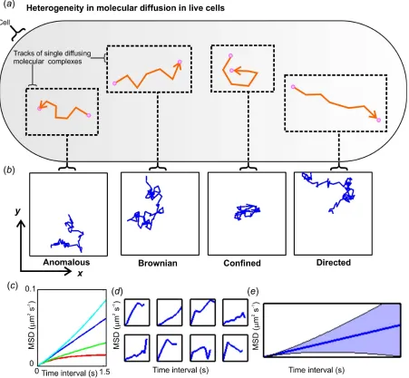
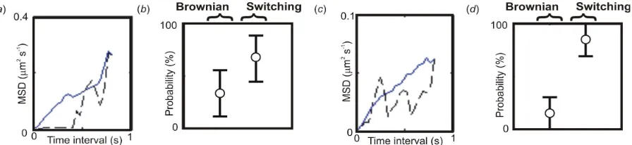
Four principal different diffusive modes are illustrated schematically in figure 1a, b with figure 1c plotting idealized mean square displacement (MSD) versus time interval

t [25]. Brownian motion represents “normal” diffusion and is the simplest mode of

diffusion characterized by a linear relation between MSD and t. However, a tracked

protein trajectory for which the MSD reaches an asymptote at high t is indicative of

confined diffusion, suggesting that the tracked protein is being trapped by its local environment - such corrals have been hypothesized as being important to forming nanoscale reaction chambers thereby greatly enhancing chemical efficiency [4, 9,

26-28]. Directed motion has an upwardly parabolic MSD function versus t and is seen for

between 0 and 1; this mode may, for example, represent the percolation of a protein through the disordered media of the membrane, hopping across corrals or interactions with specialized domains [32-35].

What is apparent from the in vivo single particle tracking studies that have

emerged over the past decade is that diffusion of molecules and complexes in living cells is in general not simple when viewed over the broad time scale of milliseconds to seconds relevant to many essential biological processes, and the reason for this may be fundamentally linked to critical sub-structural features of cells which are characterized over a length scale of a few to several hundred nanometres. There is therefore a compelling biological need to try to understand these complex diffusive processes.

Several analytical approaches have been attempted for characterizing diffusion in the cell membrane in addition to standard Saffman-Delbrück modelling, often involving heuristic approaches [11, 36]. A common approach has been to measure the ratio of the MSD with that expected from simple Brownian motion, embodied by a “relative deviation” parameter [26]. For directed motion, this parameter increases with t,

whereas for confined motion, it decreases. However, these types of MSD analysis approaches are weak on several levels when applied to tracks generated from FP-tagged molecular complexes in vivo. Firstly, trajectories are determined from a low

signal-to-noise ratio environment in which only tracks of short duration are able to be measured due primarily to the poor photophysics of the fluorophore resulting in scant, imprecise MSD information at high t [37]. Secondly, trajectories are generated from a

stochastic process, implying significant deviations from the idealized graphs of figure 1c.

In addition, this method is highly reliant upon an accurate measurement of the diffusion coefficient, which in the noisy, heterogeneous environment of the cell membrane may prove very challenging.

An appeal of MSD analysis lies in its relative simplicity to address qualitative questions concerning the membrane environment, for example effects of molecular crowding or confinement [38, 39]. However, as figure 1d, e illustrate there is an

curve from a single particle trajectory. Population averaging can smooth out such variation to obtain average behaviour, but with the unfortunate result that we lose informative data concerning the biological heterogeneity of the ensemble of diffusing molecular complexes. Recent improvements to MSD analyses have involved applications of some diffusion propagators directly. The propagators define the probability distributions that a diffusing particle will be at a given distance from its origin after a given time. These methods have been used in estimating cumulative probability distributions to substantiate the presence of different non-Brownian diffusive modes [33, 40, 41].

Our new approach here is to present an inference scheme that can separate the distinct types of diffusive modes of individual trajectories without population averaging, and do so in a probabilistic fashion, given conditions imposed on real experimental data. This can then be combined with photophysical information to quantify molecular stoichometry of diffusing complexes thus allowing probing of non-trivial relations between the size of a molecular complex and how fast it moves in vivo. The inference of these diffusive modes is done using a Bayesian

approach, incorporating a priori knowledge, based on both simulation and

experiment. We denote this as Ba yesian r anking of d iffusion (BARD).

Our study outlines the principles of the inference in light of the theory of diffusive processes. We describe the details of simulation using the different diffusive modes, and the inference algorithm used in separating out diffusive modes in a quantitative, probabilistic manner. We validate the inference using realistic simulated data, and apply to two different cell strains expressing FP fusion constructs to different membrane proteins. We obtain these live-cell data using TIRF microscopy. One cell strain expresses a single transmembrane helix probe in the cell membrane with a GFP fusion protein. The second strain is a yellow fluorescent protein (YFP) fusion to single twin-arginine translocation (Tat) protein complexes expressed in the cytoplasmic membranes of living bacteria, which exhibit significant real heterogeneity in terms of molecular stoichiometry, architecture and mobility.

2. MATERIALS AND METHODS

(a) Bacterial cell strain and preparation

Two different Escherichia coli strains were used in our in vivo microscopy investigations.

One was cell strain AyBC, as studied previously [11], using identical cell preparation conditions. This represents a heterogeneous, oligomeric membrane protein system. The cell strain contained a construct specifying a C-terminal enhanced YFP tag (Clontech Laboratories Inc., Mountain View, CA) to the native E. coli protein TatA on the

cytoplasmic side of the membrane. The Tat system of bacteria translocates natively folded protein substrates across the cytoplasmic membrane through a nanopore whose walls are composed of subunits of the TatA protein (figure 2a). In addition to TatA, there

are two other essential proteins in the Tat system, TatB and TatC, implicated both in substrate recruitment and gating of the TatA nanopore (figure 2b).

A second fusion construct was also investigated, denoted Helix1021-GFP (figure 2b). This represents a far less complex membrane protein system, which

consisted of just a simple model membrane protein of a single membrane-spanning alpha-helix fused to a GFP tag on the cytoplasmic side of the membrane [42]. The fusion gene coding for this model membrane protein used the open reading frame

sll1021 in the cyanobacterium Synechocystis sp. PCC6803 as a start point, but

expressing this as a membrane protein in E. coli for which there were no identified

orthologues. The protein has an undetermined function but has been identified in the

plasma membrane of Synechocystis [43], with the predicted gene product consisting of

673 amino-acids with a single predicted transmembrane alpha-helix close to the N-terminus. A portion of the sll1021 sequence coding for 38 amino-acids including the

predicted transmembrane alpha-helix was fused in-frame to the gene coding for GFPmut3* [44] with a linker of 5 asparagine residues. This construct was expressed in

E. coli cells from the arabinose-inducible pBAD24 vector [45], with a predicted topology

Cells of both strains were grown in Luria-Bertani (LB) medium [46] aerobically with shaking overnight at 37°C, and supplemented with 50 μg/ml ampicillin for correct antibiotic-resistant colony selection. Cells were diluted by 1:100 from the saturated cultured into M63 minimal media for sub-culturing, and were grown to mid-exponential phase typically for 3.5 hours at 30°C. For the Helix1021-GFP strain, L-arabinose was added to the culture at a final concentration of 2 mM. Cells were injected into a 5-10 µl flow-cell with poly-L-lysine-coated glass coverslips as the lower surface, allowed to settle for 10 min, washed with excess M63 and incubated with a 0.1% suspension of 202 nm diameter latex microspheres (Invitrogen Ltd., Paisley, UK) for 2 min to mark the coverslip surface, and washed with excess M63 buffer.

(b) TIRF microscopy and single particle tracking

A home-built inverted TIRF microscope was used with either a 473 nm laser for GFP excitation, or a 532 nm excitation wavelength for YFP excitation, with excitation intensity in the range 250-500 W cm-2 _{and measured depth of evanescent field penetration}

110 ± 10 nm, with specifications as described previously[7, 11, 28, 47-50], using either

473 nm or 532 nm laser dichroic mirrors and notch-rejection filters (Semrock) as appropriate. The focal plane was set at 100 nm from the coverslip surface to image the cell membrane conjugated to the glass coverslip. Fluorescence emission was imaged at ~40 nm/pixel in frame-transfer mode at 25 Hz by a 128x128-pixel, cooled, back-thinned electron-multiplying charge-coupled device camera (iXon+ DV860-BI, Andor Technology). Images were sampled for typically ~8 s. Fluorescent particle positions on each time-stamped image frame were detected and fitted using automated custom-written image-analysis software which fitted a two-dimensional radial Gaussian function plus planar local background to the image intensity data for each candidate particle.

molecules, and down to 5-10 nm for molecular complexes/assemblages containing more typically ~tens of FP molecules.

Tracks were generated from each particle provided tolerance criteria in subsequent image frames were satisfied on the basis of size, intensity and position of detected particles in subsequent image frames, for at least five consecutive image frames. The MSD versus time interval relation was then calculated for each particle trajectory, as described previously [11]. Using a Fourier spectral approach we were able to estimate the stoichiometry of these complexes through step-wise photobleaching of the relevant fluorescent protein molecule [7].

(c) Implementing and validating the BARD algorithm

Generation of synthetic tracks for validation. Two-dimensional simulated tracks for

use in validation were generated in a standard way by a stochastic random walk process in MATLAB (The MathWorks, Natick, MA) to approximate real diffusion for the fluorescently-labelled proteins in cytoplasmic membranes of E. coli cells, sampling at

the same 40 ms video-rate time interval as for experimental imaging, with track durations of typically 0.8 s (see figure S1, Supplementary Material).

Bayesian formulation. The general principle of Bayesian inference is to quantify

the present state of knowledge and refine this on the basis of new data, under-pinned by Bayes’ theorem, emerging from the definition of conditional probabilities

(fur-ther details, see Supplementary Material). In words this is simply: Posterior=(Likelihood x Prior)/Evidence

There are two stages in our statistical inference; parameter inference and model se-lection. Both use an application of Bayes’ Theorem. The first stage infers the pos-terior distributions about each model parameter, which is defined as:

( ) ( | ,₍ ) (₎ | ) | ,

|

P d w M P w M P w d M

P d M =

.

Here, M is a specific diffusion model, w is a model parameter and d represents SPT

data, and a phrase “P(A|B)” means “the probability of A occurring given that B has

single model, M. Both the posterior and likelihood are conditioned upon the data d.

We can now explain the three names of the terms above:

• The likelihood, P(d|w,M): the probability distribution of the data for a

given parameter.

• The prior, P(w|M): the initial distribution prior to any conditioning by

the data. Priors embody our initial estimate of the system, such as distribution of the parameters or the expected order of magnitude.

• The posterior, P(w|d,M): the distribution of the parameter following the

conditioning by the data.

The second stage in our statistical inference is model selection. This invokes anoth-er application of Bayes’ Theorem:

( ) ( | _{( )}) ( )

| P d M P M

P M d

P d =

.

P(M|d) is a number which is the model posterior, or probability. P(M) is a number

which is the model prior, P(d|M) is a number which is the model likelihood and P(d)

is a number which is a normalising factor which accounts for all possible models. This now generates the posterior (i.e. probability) for a specific model.

Linking the two stages in our statistical inference is the term P(d|M), the

mod-el likmod-elihood. This is also the normalisation term in the first stage. As modmod-el priors are usually flat (i.e. all models are expected equally), P (d|M) is often referred to as

the “evidence”, a portable unitless quantity. In the general case, comparing the P (d|

M) values for each independent model allows us to rank and select models

(Supple-mentary Material)

Diffusion Models. As proof-of-principle, we used four standard diffusion models

which are typical of observed molecular scale motion in living cells (Tables S1 and S2, Supplementary Material). These were Brownian, anomalous, confined and directed diffusion, and we used the underlying propagators associated with each different diffusion model directly (full details in Supplementary Material).

Inference in BARD. The inference scheme was split into two forms. One uses the

directly on the individual frame-by-frame spatial displacements measured for each

track, which we call the PDF method. These form the likelihoods, P(w|d,M)

(Supplementary Material).

As discussed in the Results section, the PDF method performed more accurately in many applications for comparing just two different non-confined diffusion models, such as anomalous diffusion with Brownian, but could not be applied to cases of confined diffusion, in which circumstance the MSD method was applied. Both approaches result in an estimate for the preliminary likelihood associated with each given single particle track.

The prior distribution for the diffusion coefficients D for Brownian diffusion,

and the equivalent transport coefficient Kα for anomalous diffusion, were modelled

as Gamma distributions (Supplementary Material, and see ref. [51] for a discussion of using a Gamma distribution). The prior distributions for the effective characteristic confinement radius R for the confined diffusion model, and for the

mean drift speed v for the directed diffusion model, were both approximated as

exponential distributions with expected sizes in the range of values that had been measured from several earlier studies in other biological systems (see Table S3,

Supplementary Material). The α factor in the anomalous diffusion model was

assumed to be uniform (i.e. flat) in the range 0.5-1.0 without further modelling.

We have no a priori expectations to indicate how this factor would be distributed.

The literature at present suggests multiple models of sub-diffusion, so the sensible consensus prior in light of this would be flat. However, an extension would be to discriminate between these different families. Either way, our uniform assumption can account for the experimental observations of anomalous diffusion with an anomalous coefficient of ~0.7-0.8.

BARD Implementation. To implement our BARD algorithm, the following steps

were taken:

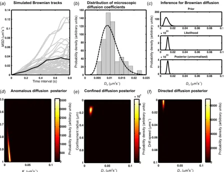
1. Quantify all of the microscopic diffusion coefficients, Dm, from the single

particle tracking data (shown here for simulated Brownian diffusion tracks in figure 4a). Here, Dm gives a measure of the short time scale rate of

individual track using the first four data points (full details in Supplementary Material).

2. Fit a Gamma distribution to the distribution of all Dm (figure 4b) and use this fit

to generate the two characteristic shape parameters of this function. Then use these shape parameters to generate the diffusion coefficient prior (see Equation

S11 and S12, Supplementary Material, and figure 4c, top panel).

3. Calculate the other parameter priors for α, R and v for the anomalous, confined

and directed diffusion models (Table S3, Supplementary Material).

4. For each separate single particle track we then calculated the likelihood (either

using Equation S8 for the PDF method, or Equation S9 for the MSD method, see Supplementary Material).

5. We then estimated the unnormalized posterior for each single particle track

against each diffusion model, taken for the pure Brownian diffusion model as:

Posterior = Likelihood(Brownian propagator) x Prior(Dm)

For the anomalous diffusion model as:

Posterior = Likelihood(anomalous propagator) x Prior(Kα) x Prior(α)

For the confined diffusion model as:

Posterior = Likelihood(confined propagator) x Prior(Dm) x Prior(R)

And for the directed diffusion model as:

Posterior = Likelihood(directed propagator) x Prior(Dm) x Prior(v)

An example of the unnormalized Brownian model posterior distribution for a typical simulated track is shown in figure 4c, lower panel. The posteriors for

the other diffusion models are shown for the same example track in figure 4d- f.

6. Normalize the parameter posterior distributions from stage 4 (details in Supplementary Material, equation S4), calculating the evidence term. This is the final step in the parameter inference section, which bridges to the second inference stage (i.e. model selection).

7. Model selection: Calculate the model posterior. Rank the models on the basis

models investigated: P(M|d). For example, for the example track shown in

figure 4a, which was simulated using a pure Brownian diffusion propagator

function, the inference ranking probabilities which were generated from the four candidate diffusion models of anomalous, Brownian, directed and confined are 33.1%, 65.6%, 1.1% and 0.2% respectively, and so in this instance Brownian diffusion is the favoured model. This is not to say that the absolute probability that the Brownian diffusion model is the correct one is ~66%, but rather that it has the highest probability of being true from the set of candidate models investigated.

8. For the top-ranked diffusion model for each single particle track we then automatically locate the centroid of the posterior, to indicate the specific value of the transport parameter for that particular diffusion model. This is done using a Gaussian fit about the posterior peak.

9. Repeat this process for all single particle tracks in the data set.

Modelling mobility changes due to switches in diffusion coefficient.

In order to demonstrate that the framework presented here can be extended to even more complicated cases of heterogeneous diffusion environments, we simulated a change in lateral diffusion coefficient as might be experienced by a single molecular complex undergoing transitions to multiple kinetic states. This may occur in signalling systems with transitions between ligand-bound and unbound states, or be due to a change in lateral mobility due to interactions with the underlying membrane such as local changes in viscosity [16] or interactions with the membrane cytoskeleton.

3. RESULTS

(a) TIRF microscopy on live bacterial cells

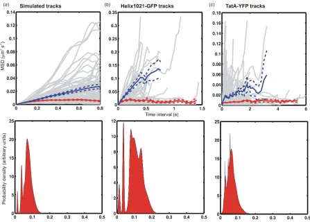
Bespoke video-rate TIRF microscopy at 40 ms per frame (figure 3a) was performed on

in width. This was larger than we measured for the point spread function width from single fluorescent protein molecules immobilized to the surface of the coverslip by ~100 nm [7]. The measured point spread function width of single FP molecules of ~200-300 nm is equivalent to the optical resolution limit of our microscope and is an inevitable feature due to diffraction of emitted fluorescence when the detector, in our case an EMCCD camera, is physically more than a few wavelengths distance away.

The TatA system had been characterized previously using epifluorescence microscopy that indicated multiple spots per cell (mean of ~15) with a range of fluorescence intensities, diffusing over the cytoplasmic membrane surface [11]. Our aim in the present study was to use TIRF illumination to improve the imaging contrast sufficiently to generate single particle trajectories in the TIRF evanescent field in the specimen focal plane, corresponding to localization of either the Helix1021 or TatA in the cytoplasmic membrane. This would then permit analysis of the transport properties of these proteins at the single molecule/single molecular complex level for a relatively simple membrane protein probe at one extreme and for a complex heterogeneous membrane protein molecular complex at the other, both in functional, living cells.

Using automated single particle tracking [11] we were able to track individual fluorescent spots to a super-resolution precision of ~40 nm or less. Experimental single particle tracks were collated and MSD values estimated (full details in Supplementary Materials). The longest duration tracks lasted typically ~1 s, but in most cases the tracks were shorter, with ~10 data points per track being more typical.

For the TatA-YFP data, cells contained typically ~2-3 fluorescent spots in TIRF

images (figure 3b), suggesting ~12-18 spots per cell since the TIRF evanescent field of

our microscope we estimate encapsulates roughly 1/6 of the E. coli cell membrane.

Most MSD traces indicated putative evidence for Brownian diffusion, with typical values of D ≈ 0.01 µm2 s-1. This was consistent with the earlier investigation, but with

The Helix1021-GFP cells contained typically ~4-6 fluorescent spots per TIRF

image (figure 3c), suggesting more like ~30 spots in total in the whole cell membrane.

MSD data again indicated putative evidence for two populations in terms of diffusive modes, one of Brownian diffusion with typical values of diffusion coefficient higher by factor of ~5-10 than the TatA-YFP data, and the other mode again qualitatively suggesting confined diffusion.

(b) Model ranking and parameter estimation

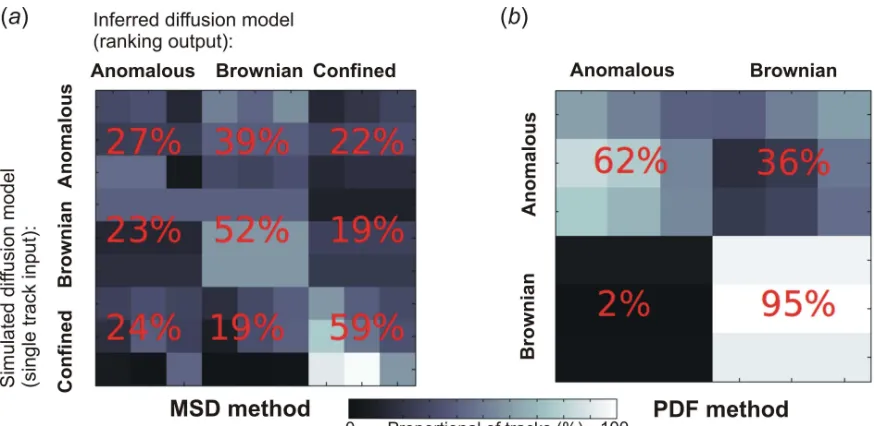
To validate our approach we tested the inference method using realistic simulated two-dimensional SPT input data utilizing mobility parameters with characteristic values comparable to those estimated qualitatively for the experimental Helix1021-GFP and TatA-YFP data from the MSD plots. We then analyzed both the parameter estimates and model rankings outputs. The correctness of the

model ranking was assessed by classification matrices. A classification

matrix represents different “input” simulated diffusion models down the rows,

i, while the different “output” diffusion models from the ranking inference are

represented across the columns, j, and then each location in the matrix is

given an associated number for the percentage of tracks that are included in that particular (i, j) class combination.

In figure 5 we show the results of two example classification matrices, one

corresponding to likelihood estimation using the MSD method in figure 5a, the other

to the PDF method in figure 5b. Previous experiments on other biological systems

which involve examples of directed diffusion, for example with putative protein treadmilling studies in vivo [29], suggested different values for characteristic

diffusion coefficients, and so directed diffusion model ranking was done separately (Supplementary Material). In this case, we investigated a range of different drift

speeds from 1-20 nm s-1_{. This indicated that at typical drift speeds used the directed}

diffusion model can be correctly identified against a Brownian model with a relative probability of ~60-70%.

identification of anomalous behaviour was poorer (~30%), probably because subtle sub-diffusive behaviour is not apparent for such typically short track lengths of only 10-20 data points as used here. The inference output for confined diffusion in particular was unsurprisingly found to be a function of track length, with the 50% threshold of correct inference for tracks being composed of at least ~16 data points (figure S2, Supplementary Material), though the change in correct relative inference probability for confined diffusion was found to be only a few % when the confinement radius was varied across a relatively large range 50-200 nm in estimating the posterior distribution. This is not to say that the choice in prior function has little effect on the final outcome; if we use a naïve “flat” prior function for the confined diffusion model (in effect, taking an infinitely large value for the confinement radius) then we estimate that the correct relative inference probability is over 20% lower compared against the non-flat priors used. In other words, utilizing physically sensible prior functions makes a substantial difference to correctly inferring the underlying type of diffusion (see Supplementary Material)

The PDF method is an approach which utilises information from the relative

dis-placements of a tracked molecule or complex from frame to frame, and so can not be applied to a confined diffusion model without a priori knowledge of the absolute position

of the diffusing particle relative to the boundaries of the putative confinement zone,

which in general is not the case. Therefore, for the PDF method we display in figure 5b

the relevant classification matrix between just anomalous and Brownian diffusion mod-els. Here, anomalous diffusion was correctly discriminated with an accuracy of at least 62%, performing better than the MSD method for corresponding diffusion models (for example, Brownian diffusion was correctly identified with a relative ac-curacy of 95% using the PDF method compared with 52% for the MSD method).

(c) Identifying switches in molecular mobility

example, be due to either a dramatic change in lipid viscosity for the micro- or nanoscale environment in which a protein molecule or complex is diffusing, or conversely through a rapid oligomerization or molecular assembly process of the diffusing complex. In this simple generalization, we assumed that the time scale of the transitional step between different lateral diffusion coefficients was much less than the sampling period. For simplicity, we assumed that diffusing particles make this mobility switch at the halfway point of their full simulated trajectory. At this point, particles were assumed to switch to a higher diffusion coefficient (from 0.01 µm2 _s-1 _{to either 0.05 µm}2 _s-1_{or 0.10 µm}2 _s-1_{), assuming true Brownian}

diffusion in each case and a video-rate sampling time interval of 40 ms for which the

number of data points in each half of a trajectory is N = 10.

A switching inference model was formulated by separating the

displacement data at each time point and allowing for two separate mobility measurements to be inferred either side of this. Figure 6 illustrates the typical simulated individual and time-averaged MSD outputs with model ranking predictions. This relatively simple switching inference modification can correctly predict switching behaviour characterized by two separate microscopic diffusion coefficients over a simple Brownian diffusion mode characterized by just a single microscopic diffusion coefficient, with a relative ranking probability in the range 65-85%, depending upon the size of the switch in diffusion coefficient. Using the PDF approach under the same conditions generated a slight improvement to correct identification, and in doing so we found that the correct switching model was identified in preference to simple Brownian motion (that is, a ranking probability in excess of 50%) down to as small a change as ~3-fold in the microscopic diffusion coefficient.

(d) Application of BARD to live-cell experimental data

Preliminary inspection of the MSD traces generated from automated single

particle tracking from both the Helix1021-GFP and the TatA-YFP E. coli cell

characterized by putatively asymptotic MSD versus time interval traces, which could be indicative of two possible populations corresponding predominantly to Brownian diffusion and confined diffusion. In the first instance, we ran a BARD analysis using all four standard diffusion models of anomalous, Brownian, confined and directed diffusion, which clearly indicated for both cell strains that Brownian and confined were the two most inferred diffusion models. We then pooled the combined inferred results from anomalous, Brownian and directed diffusion as constituting “mobile” tracks, and compared this to the inferred confined track data on MSD versus time interval plots.

Simulated realistic track data using our standard set of mobility parameters (Table S3, Supplementary Material) indicated that a mixture of such mobile and confined tracks could be successfully discriminated, with both the imposed values for microscopic diffusion coefficient and confinement radius agreeing with those

inferred from the BARD analysis to within the measurement error (Figure 7a).

Applying BARD analysis to the Helix1021-GFP track data indicated that 50-60% of all tracks exhibited confined diffusion with an estimated confinement radius of 110 ± 50 nm (± s.d.), with the mobile population characterized by a

microscopic diffusion coefficient typically in the range 0.01-0.05 µm2 _s-1

(Figure 7b). BARD analysis applied to the TatA-YFP track data indicated a

smaller but still significant proportion of 30-40% of all tracks exhibiting confined diffusion with a mean confinement radius of 60 ± 40 nm, and the mobile population characterized by a smaller typical microscopic diffusion coefficient in the range 0.002-0.01 µm2 _s-1 _{(Figure 7c).}

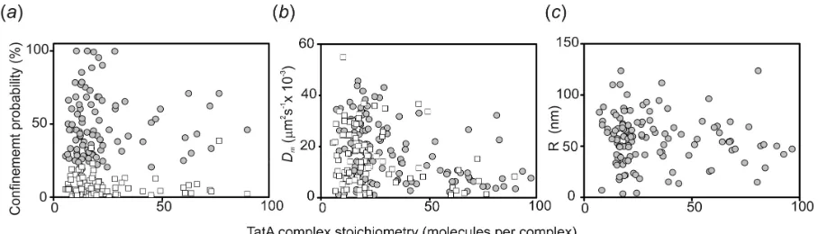
molecules per spot, whereas that of the confined population was higher by ~50% (figure 8a). We saw no obvious differences in microscopic diffusion coefficient

between the confined and mobile populations (figure 8b) nor of any clear

correlation between molecular stoichiometry in each fluorescent spot and the

inferred size of the confinement radius (figure 8c).

4. DISCUSSION

The ability to monitor single molecules or complexes diffusing in living cells is an excellent example of the “next generation” single-molecule cellular biophysics approaches which have emerged over the past decade. What some researchers are now trying to do with such exceptionally precise molecular-level data is to use them to increase our understanding of the functional architecture of both the diffusing molecules themselves and of their local cellular environment. However, to do so requires a development of novel computational methods that can accurately measure the underlying modes of diffusion from the typically noisy and limited data from these tracked molecules in vivo.

Two approaches were investigated, one using the MSD and the other using the PDF method. In each case, a prior formulation was used to describe the expected distribution of the parameters. Although neither approach could effectively discriminate between anomalous and confined modes of motion, which from the MSD curves have qualitatively similar shapes for noisy short tracks, we find that the PDF and MSD methods in tandem have different resolving power. The MSD method effectively identifies confined from simple Brownian motion, whereas the PDF method effectively identifies anomalous diffusion from Brownian diffusion. In addition, the PDF approach has a strong resolving power in that it can identify dynamics within a single track, as observed in the simulations of diffusion coefficient switching.

The PDF method does not take into account the full effect of experimental noise, as distinct from random fluctuations due to the stochastic nature of the diffusion processes. Levels of experimental noise are likely to vary between different experimental equipment and need to be properly characterized for each individual case. However, this was qualitatively incorporated into the MSD approach, where Gaussian errors are assumed. Experimental noise, arising in tracking would be included in the error, and would add by quadrature to the expected fluctuations due to stochastic noise (the time interval zero point in our case assumes an MSD error of around 40 nm2_).

Our in vivo video-rate particle trajectories contain approximately 10-30 times

fewer data points than those used in previous studies utilizing tracking of gold particles [4, 26, 27, 53], organic dye labelling of clusters containing hundreds of molecules [39] or quantum-dot tracking [41], and are of comparable duration to those obtained previously using single molecule fluorescence microscopy either in artificial lipid layers or in vivo

[11, 33, 40]. These have implemented a variety of different methodologies to analyze single particle trajectories involving either regression fitting of the MSD versus time interval relation, application of a relative deviation parameter or constructed probability distributions representative of the modes of interest.

microscopy, with typically very short tracks observed, it is generally infeasible to analyze such trajectories without some form of population averaging using conventional techniques. Exceptions are made of course to the occasional long track which is observed, or tracks which appear representative, but a majority of the body of data captured is noisy, and unrepresentative if multiple modes of behaviour are under investigation.

Our study was aimed at being able to discriminate, without population averaging, such molecular-level tracks. Once individual particle trajectories are categorized into different modes of diffusive behaviour, models can be built on how they behave collectively, potentially allowing greater physiological interpretation of the protein mobility characteristics in functional, living cells, and hence to have a greater understanding on their underlying membrane micro- and nanoscale structure in a biologically-relevant context. We have performed a validation across the approximately

biological relevant parameters for the datasets presented. However, extrapolating these

to any real system should come with the caveat that the classifications can only really be used as a guide for the particular set of algorithm parameters and system parameters used.

Ultimately, since the inference scheme is probabilistic there will inevitably be some trajectories which are falsely categorized with the wrong behaviour, most often into simple Brownian motion, as shown in the classification matrices. We included details on how model ranking varies with respect to the number of data points to demonstrate that there will often be a crossover between mis-categorization and the correct identification. A caveat then, for interpreting any model selection on the

experimental data would be that there is no evidence of heterogeneity under the given

experimental conditions. If this crossover is unreachable in the experimental framework

In an earlier single particle tracking study on the Tat system using non-TIRF illumination, the presence of an “immobile” sub-population of TatA protein complexes was reported, but not investigated further [11]. In our study, BARD analysls reveals that a significant proportion of TatA-YFP complex tracks have a confinement radius of 60 ± 40 nm. The measured localization precision on our microscope for tracking a single YFP molecule is ~40 nm. However, TatA complexes were observed to have a broad range of stoichiometry, with a median value of equivalent to ~20-30 TatA-YFP subunits, consistent with that reported previously [11]. These complexes are therefore brighter than a single YFP molecule by a factor of ~20-30, with the localization precision following iterative Gaussian fitting of the intensity profile of these fluorescent spots scaling approximately by the square-root of this factor, or ~5 (see ref. [57]), so the localization tracking precision for most TatA-YFP complexes is more like 5-10 nm. Therefore, the estimated confinement radius here is substantially higher than the localization precision for diffusing complexes, which strongly suggests that the majority of the “immobile” TatA complexes previously reported were in fact exhibiting true confined diffusion.

Similarly, we observed a significant sub-population of tracks for the Helix1021-GFP strain which exhibited confined diffusion, here with a mean confinement radius of 110 ± 50 nm, within experimental error of that measured for the TatA-YFP strain. The fact that the transmembrane helix probe has no known specific interaction

with molecular systems in E. coli suggests that the confinement domains in both

The diffusion models illustrated here are not exclusive as such – there is a risk that none of the models is actually the physically “correct” one. BARD analysis will provide probabilistic rankings of these models, but these probabilities can strictly only be interpreted in the context of the other models considered, and do not represent an absolute probability. Model selection is open-ended; the models presented here do not take into account the full degree of potential heterogeneity that may exist in the cell membrane, and other models can be considered. For example, there are several theorised models of anomalous sub-diffusion, each with a unique PDF. There may also be complex dynamic behaviour that has not been taken into account, such as hopping diffusion, reaction kinetics and molecular assembly effects. A natural extension of this BARD approach as we present it here is to incorporate more complex behaviour which may better capture the real, physiological behaviour of diffusion in living cells.

Separating different mobility characteristics into different categories will clearly facilitate insight into several important biological questions. For example, how proteins partition dynamically in the cell membrane, whether signalling events are linked to membrane architecture, the precise manner in which motor proteins shuttle in or near to cell membranes, and the extent to which interacting proteins rely upon random collisions or are part of putative confined “solid-state” reaction zones. Such new diffusion analysis tools that we report here might indeed also be further extended to larger length scale investigations beyond that of the single molecule and single cell, such as rheological or cell migration studies at the level of cellular populations in normal tissue development and tumour formation in cancer.

SUPPORTING MATERIAL

Electronic supplementary material is available via http://rstb.royalsocietypublishing.org.

ACKNOWLEDGEMENTS

bacterial cell strain AyBC, Anja Neninger and Conrad Mullineaux for the donation of bacterial cell strain Helix1021-GFP. This work was supported via a research grant to MCL (EP/G061009). MLC was supported by a Royal Society University Research Fellowship. AR was supported by the Research Councils UK.

REFERENCES

1 Singer, S. J., & Nicolson, G. L. 1972. The fluid mosaic model of the structure of

cell membranes. Science175, 720–731

2 Jacobson, K. E., Sheets, E. D. & Simson, R. 1995. Revisiting the fluid mosaic

model of membranes. Science 268, 1441-1442

3. Vereb, G.J., Szollosi, J., Matko, J., Nagy, P., Farkas, T., Vigh, L., Matyus, L., Waldmann, T. A. & Damjanovich, S. 2003 Dynamic, yet structured: The cell membrane

three decades after the Singer-Nicolson model. Proc Natl Acad Sci U S A. 100,

8053-8058

4 Kusumi, A., Nakada, C., Ritchie, K., Murase, K. Suzuki, K., Murakoshi, H., Kasai,

R. S., Kondo, J. & Fujiwara, T. 2005. Paradigm shift of the plasma membrane concept from the two-dimensional continuum fluid to the partitioned fluid: high-speed

single-molecule tracking of membrane single-molecules. Annu Rev Biophys Biomol Struct. 34,

351-378

5 Vrljic, M., Nishimura, S. Y., Brasselet, S., Moerner, W. E. & McConnell, H. M.

2002. Translational Diffusion of Individual Class II MHC Membrane Proteinsin Cells.

Biophys J. 83, 2681-2692

6. Deich, J., Judd, E. M., McAdams, H. H. and Moerner, W. E. 2004. Visualization

of the movement of single histidine kinase molecules in live Caulobacter cells. Proc Natl Acad Sci USA.101,15921-15926

7. Leake, M. C., Chandler, J. H., Wadhams, G. H., Bai, F., Berry, R. M. and

Armitage, J. P. 2006. Stoichiometry and turnover in single, functioning membrane

protein complexes. Nature.443, 355-358

8. Lommerse, P. H., Vastenhoud, K., Pirinen, N. J., Magee, A. I., Spaink, H. P. and

Schmidt, T. 2006. Single-molecule diffusion reveals similar mobility for the Lck, H-ras,

9. Wieser, S., Moertelmaier, M., Fuertbauer, E., Stockinger, H. and Schütz, G. J. 2007 (Un)confined diffusion of CD59 in the plasma membrane determined by

high-resolution single molecule microscopy. Biophys J.92, 3719-3728

10. Lee, C. L. and Petersen, N. O. 2003. The Lateral Diffusion of Selectively

Aggregated Peptides in Giant Unilamellar Vesicles. Biophys J.84, 1756-1764

11. Leake, M. C., Greene, N. P., Godun, R. M., Granjon, T., Buchanan, G., Chen, S.,

Berry, R. M. and Berks, B. C.. Variable stoichiometry of the TatA component of the twin-arginine protein transport system observed by in vivo single-molecule imaging. 2008. Proc Natl Acad Sci U S A. 105, 15376-15381

12. Saffman, P. G. and Delbruck, M. 1975. Brownian motion in biological

membranes. Proc Natl Acad Sci U S A. 72, 3111-3113

13. Hughes, B. D., Pailthorpe, B. A. and White, L. R. 1981. The translational and

rotational drag on a cylinder moving in a membrane. J. Fluid Mech. 110, 349-372

14. Lillemeier, B. F., Pfeiffer, J. R., Surviladze, Z., Wilson, B. S. and Davis, M. M. 2006. Plasma membrane-associated proteins are clustered into islands attached to the

cytoskeleton.Proc Natl Acad Sci U S A. 103, 18992-18997

15. Simons. K. and Ikonen, E. 1997. Functional rafts in cell membranes. Nature. 387,

569-572

16. Pike, L. J. 2009. The challenge of lipid rafts. J Lipid Res.50, S323-S328

17. Schmidt, T., Schütz, G. J., Baumgartner, W., Gruber, H. J. and Schindler, H.

1996. Imaging of Single Molecule Diffusion. Proc Natl Acad Sci U S A. 93, 2926-2929

18. Cheezum, M. K., Walker, W. F. and Guilford, W. H. 2001. Quantitative

Comparison of Algorithms for Tracking Single Fluorescent Particles. Biophys J. 81,

2378-2388

19. Kural, C., Kim, H. , Syed, S., Goshima, G., Gelfand, V. I. and Selvin, P. R.. 2005.

Kinesin and Dynein Move a Peroxisome in vivo: A Tug-of-War or Coordinated

Movement? Science. 308, 1469-1472

20. Geerts, H., De Brabander, M., Nuydens, R., Geuens, S., Moeremans, M. , De

Mey, J. and Hollenbeck, P. 1987. Nanovid tracking: a new automatic method for the study of mobility in living cells based on colloidal gold and video microscopy. Biophys J.

21. Schütz, G.J., Kada, G., Pastushenko, V.P. and Schindler, H. 2000 Properties of lipid microdomains in a muscle cell membrane visualized by single molecule

microscopy. EMBO J. 19, 892-901

22. Sako, Y., Minoghchi, S. and Yanagida, T. 2000. Single-molecule imaging of

EGFR signalling on the surface of living cells. Nat. Cell Biol.2, 168-172

23. Tsien, R. Y. 1998. The green fluorescent protein. Annu Rev Biochem. 67,

509-544.

24. Leake, MC. 2010.Shining the spotlight on functional molecular complexes: The new

science of single-molecule cell biology.Commun Integr Biol. 3,415-418.

25. Gross, D. J., and Webb, W. W. 1988. Cell surface clustering and mobility of the

liganded LDL receptor measured by digital video fluorescence microscopy. In

Spectroscopic Membrane Probes II, 1st ed., Loew L. M. editor, CRC Press, Boca Raton, FL. 19-45

26. Kusumi, A., Sako, Y., and Yamamoto, M. 1993. Confined lateral diffusion of

membrane receptors as studied by single particle tracking (nanovid microscopy). Effects of calcium-induced differentiation in cultured epithelial cells. Biophys. J. 65,

2021-2040

27. Daomas, F., Destainville, N., Millot, C., Lopez, A., Dean, D. and Salome, L. 2003. Confined diffusion without fences of a g-protein-coupled receptor as revealed by single particle tracking. Biophys J.84, 356-366

28. Lenn, T., Leake, M. C. and Mullineaux, C. W. 2008. Clustering and dynamics of

cytochrome bd-I complexes in the Escherichia coli plasma membrane in vivo. Mol. Microbiol.70, 1397-1407

29. Kim S.Y., Gitai, Z., Kinkhabwala, A., Shapiro, L. and Moerner, W. E. 2006. Single

molecules of the bacterial actin MreB undergo directed treadmilling motion in

Caulobacter crescentus. Proc Natl Acad Sci USA. 103, 10929-10934

30. Demond, A. L., Mossman, K. D., Starr, T., Dustin, M. L. and Groves, J. T. 2008.

31. Bouchaud, J. P. and Georges, A. 1990. Anomalous diffusion in disordered media: Statistical mechanisms, models and physical applications. Physics Reports. 195,

127-293

32. Saxton, M. 1994. Anomalous diffusion due to obstacle: a Monte Carlo study.

Biophys J.66, 394-401

33. Schütz, G. J., Schindler, H. and Schmidt, T. 1997. Single-molecule microscopy

on model membranes reveals anomalous diffusion. Biophys. J.73, 1073-1080

34. Metzler, R. 2000. The random walk’s guide to anomalous diffusion: a

fractional dynamics approach. Physics Reports. 339, 1-77

35. Nicolau, D. V., Hancock, J. F. and Burrage, K. Sources of anomalous

diffusion on cell membranes: A monte carlo study. 2007. Biophys. J. 92,

1975-1987

36. Peters, R., and Cherry, R. J. 1982. Lateral and Rotational Diffusion of

Bacteriorhodopsin in Lipid Bilayers: Experimental Test of the Saffman-Delbruck

Equations. Proc Natl Acad Sci USA. 79, 4317-4321

37. Füreder-Kitzmüller, E., J. Hesse, A. Ebner, H. J Gruber, and Schütz, G. J. 2005.

Non-exponential bleaching of single bioconjugated Cy5 molecules. Chem Phys Lett.

404, 13-18

38. Guigas, G., and Weiss, M. 2008. Sampling the cell with anomalous diffusion

- the discovery of slowness. Biophys J. 94, 90-94

39. Bruckbauer, A., Dunne, P. D., James, P. Howes, E., Zhou, D., Jones, R. and D.

Klenerman Selective diffusion barriers separate membrane compartments. 2010.

Biophys. J.99, L1-3

40. Schaaf, M. J. M., Koopmans, W. J. A., Meckel, T., van Noort, J., Snaar-Jagalska,

B. E., Schmidt, T. and Spaink, H. P. 2009. Single-molecule microscopy reveals membrane microdomain organization of cells in a living vertebrate. Biophys. J. 97,

1206-1214

41. Pinaud, F., Michalet, X., Iyer, G., Margeat, E., Moore, H. P. and Weiss, S. 2009.

Dynamic partitioning of a glycosyl-phosphatidylinositol-anchored protein in

glycosphingolipid-rich microdomains imaged by single-quantum dot tracking. Traffic.10,

42. Nenninger, A., Mastroianni, G., Robson, A., Lenn, T., Xue, Q., Leake, M. C. and

Mullineaux, C. W. 2012. Independent mobility of proteins and lipids in the plasma

membrane of Escherichia coli. Manuscript in preparation

43. Huang, F., Parmryd, I., Nilsson, F., Persson, A. L., Pakrasi, H. B., Andersson, B.

and Norling, B. 2002. Proteomics of Synechocystis sp. strain PCC6803. Identification

of plasma membrane proteins. Mol Cell Proteomics 1, 956-966

44. Cormack, B. P., Valdivia, R. H. and Falkow, S. 1996. FACS-optimized mutants

of the green fluorescent protein (GFP). Gene 173, 33-38

45. Guzman, L.-M., Belin, D., Carson, M. J. and Beckwith, J. 1995 Tight regulation,

modulation, and high-level expression by vectors containing the arabinose P-BAD

promoter. J Bacteriol177, 4121-4130

46. Sambrook, J. & Russell, D. W. 2001. Molecular Cloning: a Laboratory Manual.

Cold Spring Harbor Laboratory Press, Plainview, NY, USA

47. Lo, C.-J., Leake, M. C. and Berry, R. M. 2006. Fluorescence measurement of intracellular sodium concentration in single Escherichia coli cells. Biophys. J. 90,

357-365

48. Lo, C.-J., Leake, M. C., Pilizota, T. and Berry, R. M. 2007. Single-cell

measurements of Membrane Potential, Sodium-Motive Force and Flagellar Motor Speed in Escherichia coli. Biophys. J. 93, 294-302

49. Lenn, T., Leake, M. C. and Mullineaux, C. W. 2008. Are Escherichia coli

OXPHOS complexes concentrated in specialized zones within the plasma membrane.

Biochem Soc Trans. 36, 1032-1036

50. Reyes-Lamothe, R., Sherratt, D. J. and Leake, M. C. 2010 Stoichiometry and

architecture of active DNA replication machinery in Escherichia coli. Science. 328,

498-501.

51. MacKay, D. J. C. 2002. In Information Theory, Inference and Learning

52. MacKay, D. J. C. 1991. Bayesian interpolation. Neural Computation. 4,

415-447

53. Qian, H., Sheetz, M. P. and Elson, E. L. 1991. Single particle tracking. Analysis

of diffusion and flow in two-dimensional systems. Biophys J.60, 910-921

54. Barkai, E., Metzler, R. and Klafter, J. 2000, Physical Review. E, 61, 132-138

55. Bickel, T. 2006. A note on confined diffusion, Physica A,377, 24-32

56. Das, R., Cairo, C,W. and Coombs, D, 2010. A Hidden Markov Model for Single

Particle Tracks Quantifies Dynamic Interactions between LFA-1 and the Actin Cytoskeleton, PLoS Comput Biol, 5, 11

57. Thompson, R. E., Larson, D. R. and Webb, W. W. 2002. Precise nanometer

Figure 1. The complexity of molecular diffusion in living cells. (a), Schematic of diffusion

(orange track) of a single molecule or complex (pink circle) in a live cell with (b)

simulated data for the typical spatial localizations of tracked molecules in the specimen

xy plane of a typical optical microscope illustrating four common modes of diffusion. (c)

Idealized forms of mean square displacement (MSD) relations for anomalous (green),

Brownian (blue), confined (red) and directed (cyan) diffusion. (d) Typical simulated

Brownian diffusion MSD data for different diffusing molecules modelled with the same

diffusion coefficient and (e) the mean average of many simulated MSD relations (blue

Figure 2. Schematic of (a) membrane bound architecture of a Twin-Arginine

Translocase TatA nanopore allowing translocation of a full folded protein substrate

across the cytoplasmic membrane, and of (b) the TatA-YFP, TatB, TatC and

Figure 3. In vivo TIRF microscopy on live bacteria. (a) Schematic of TIRF on an E. Coli

cell immobilized to a glass microscope coverslip. False-colour TIRF images on single cells for the (b) TatA-YFP and (c) Heli1021-GFP cell strains, cell outline indicated

Figure 4. Implementing BARD. (a) Simulated Brownian tracks (grey) all with diffusion

coefficient D=0.01 µm2 s-1, with one of these tracks highlighted (black) for BARD

analysis. (b) Distribution of measured microscopic diffusion coefficient Dm values from

tracks in (a) with Gamma fit indicated (dashed line). (c) Constructing probability

distributions used in BARD for the highlighted track of (a) tested against a Brownian diffusion model showing the unnormalized prior (upper panel), likelihood (middle panel) and posterior (lower panel). Testing against the three other diffusion model generates two-dimensional unnormalized posterior distributions for (d) anomalous, (e) confined

and (f) directed diffusion models. For the highlighted track shown in (a) the highest

Figure 5. Characterizing the error in the BARD analysis using classification matrices for

(a) the MSD method, and (b) the PDF method. Each “pixel” in the matrix represents a

combination of a type of simulated track against an inferred highest ranked diffusion model from the BARD analysis, with greyscale indicating the individual inference ranking percentage. Each diffusion mode here was simulated with three different tracks, and therefore each matrix is composed of individual 3x3 sub-matrices, with the percentage in red indicating the mean average inference ranking percentage within that sub-matrix. Thus, the “diagonal” of (a) and (b) constitutes the “”true-positive”

Figure 6. Inferring a sudden change in diffusion coefficient. (a) MSD relation for a single

track simulated assuming Brownian diffusion (black) and the mean average of 20 such

tracks (blue) for which the diffusion coefficient D switches from 0.01to 0.10 µm2 s-1, with

(b) associated ranking inference probabilities for a single D Brownian (B) and two D

Switching (S) model. (c) MSD relation for a single track (black) and average of several

tracks (blue) for which D switches from 0.01 to 0.05 µm2 s-1 , with (d) associated ranking

Figure 7. Comparing mobile and immobile tracks. Upper panels are MSD versus time interval traces showing mean values assuming at least n=3 data points at each time

interval value, for all “mobile” tracks (blue, solid line) and confined tracks (red, solid line), s.e.m. error bounds shown (dotted lines), individual tracks shown in grey, for (a)

simulated tracks (n=50 mobile tracks here simulated using a Brownian diffusion

propagator function, n=50 confined tracks), (b) Helix1021-GFP (n=20 mobile tracks, n=27 confined tracks) and (c) TatA-YFP (n=258 mobile tracks, n=164 confined tracks).

Figure 8. Variation in (a) the probability that the top ranked diffusion mode will be

confined, (b) the microscopic diffusion coefficient Dm and (c) the confinement radius R

Supporting Material

Inferring diffusion in single live cells at the single

molecule level

Alex Robson,Kevin Burrage,and Mark C. Leake*

Generation of synthetic tracks

2D simulated tracks were generated using a stochastic random walk process, generated in MATLAB (The MathWorks, Natick, MA). This algorithm modelled the stochastic Ito differential equation:

dX=F(X ,t)dt+

√

Here, X is simulated particle displacement for a given spatial dimension as a function

of time t, F is a function that represents drift, G is a function that represents

diffusion and dW represents an incremental Wiener process. Following an

incremental sampling time δt, X changes its amount by a value δX which is

normally distributed such that <δX> ≈ F(X,t)δt and the variance

Var(δX) ≈ 2DG(X,t)TG(X,t)δt, where D is the corresponding lateral diffusion

coefficient. For Brownian, confined and directed diffusion, appropriate conditions on

F and G were chosen (Table S1) using a video-rate sampling time of 40 ms

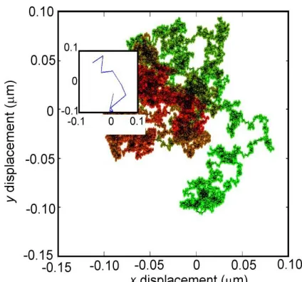
throughout to predict random incremental displacements for a simulated particle track. Anomalous motion was simulated separately, by rejection sampling of the probability distribution but used essentially the same randomized, incremental process. For confined tracks, the domain was modelled as an harmonic potential well in which a particle at the domain edge experiences a forcing function F that drives it back into the

domain, similar to the approach in [58] (Figure S1). We simulated anomalous diffusion through a rejection sampling algorithm.

Table S1. Selection of drift and diffusion functions in the stochastic equation

Mode F(X,t) G(X,t)

Brownian 0 1

Directed >0 1

Confined -sign(X) if X≥L;

0 if X<L

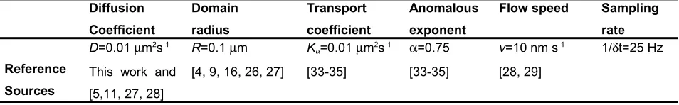
Figure S1. Simulated confined diffusion. Displacements in xy of a highly sampled confined track. Colouring added to indicate procession with time

proceeding from red at the origin to light green. Inset shows the observed

track with just N = 10 data points at video-rate sampling. Confinement

radius R = 0.1 µm.

Bayesian formulation

The general principle of Bayesian inference is to quantify the present state of

knowledge and refine this on the basis of new data, underpinned by Bayes’ theorem,

emerging from the definition of conditional probabilities. This can be explained by

considering the probability of two general events, A and B, happening, which is denoted P(A∩B), which equates to the probability of B happening, P(B), multiplied by the

probability of A given that B has occurred, denoted P(A│B), or: P(A∩B)=P(A│B)P(B)

Using the same notation we can say that:

P(B∩A)=P(B│A)P(A)

Since these two equations are equal this leads to Bayes’ theorem of:

P(A│B)= P(B│A)P(A)/P(B) (S1)