A spatial microsimulation approach for the analysis of commuter patterns: from individual to regional levels

This is a repository copy of

A spatial microsimulation approach for the analysis of

commuter patterns: from individual to regional levels

.

White Rose Research Online URL for this paper:

http://eprints.whiterose.ac.uk/77369/

Version: Published Version

Article:

Lovelace, R, Ballas, D and Watson, M (2014) A spatial microsimulation approach for the

analysis of commuter patterns: from individual to regional levels. Journal of Transport

Geography, 34. 282 - 296. ISSN 0966-6923

https://doi.org/10.1016/j.jtrangeo.2013.07.008

[email protected]

https://eprints.whiterose.ac.uk/

Reuse

Unless indicated otherwise, fulltext items are protected by copyright with all rights reserved. The copyright

exception in section 29 of the Copyright, Designs and Patents Act 1988 allows the making of a single copy

solely for the purpose of non-commercial research or private study within the limits of fair dealing. The

publisher or other rights-holder may allow further reproduction and re-use of this version - refer to the White

Rose Research Online record for this item. Where records identify the publisher as the copyright holder,

users can verify any specific terms of use on the publisher’s website.

Takedown

If you consider content in White Rose Research Online to be in breach of UK law, please notify us by

A spatial microsimulation approach for the analysis of commuter

patterns: from individual to regional levels

q

Robin Lovelace

_{, Dimitris Ballas, Matt Watson}

Department of Geography, The University of Sheffield, Sheffield S10 2TN, United Kingdom

a r t i c l e

i n f o

Keywords:

Spatial microsimulation Commuting

Policy evaluation

a b s t r a c t

The daily trip to work is ubiquitous, yet its characteristics differ widely from person to person and place to place. This is manifested in statistics on mode and distance of travel, which vary depending on a range of factors that operate at different scales. This heterogeneity is problematic for decision makers tasked with encouraging more sustainable commuter patterns. Numerical models, based on real commuting data, have great potential to aid the decision making process. However, we contend that new approaches are needed to advance knowledge about the social and geographical factors that relate to the diversity of commuter patterns, if policies targeted to specific individuals or places are to be effective. To this end, the paper presents a spatial microsimulation approach, which combines individual-level survey data with geographically aggregated census results to tackle the problem. This method overcomes the limitations imposed by the lack of available geocoded micro-data. Further, it allows a range of scales of analysis to be pursued in parallel and provides insights into both the types ofareaandindividualthat would benefit most from specific interventions.

Ó_{2013 The Authors. Published by Elsevier Ltd. All rights reserved.}

1. Introduction

Commuting is a major reason for personal travel,1_{and a broad}

research area within transport geography. In many cases zonally aggregated census statistics—often the most reliable source of infor-mation about spatial variation in commuter patterns—form the basis of geographical commuting research (Horner and Murray, 2002; Titheridge and Hall, 2006). Recent advances in data availability and computational methods have, however, facilitated the analysis (Helminen and Ristimäki, 2007) and modelling (Buliung and Kanaroglou, 2002; Buliung and Kanaroglou, 2006) of commuting at individual and household levels. This trend—towards micro-level social and spatial analysis—has several potential benefits for decision makers, including:

The ability to target specifictypesof commuters.

The potential to model the impacts of small-scale interventions

(e.g. a new bicycle path) on individuals living in the local area.

Higher spatial resolution, allowing for realistic insight into the

impacts of change on network usage (e.g. identify likely points of congestion).

The results provide a foundation for agent-based and dynamic

microsimulation models.

The shift towards micro-level analysis also has some potential disadvantages. These include greatly increased computational requirements for analysis, lack of available software or expertise, and the pitfalls of overcomplexity. As recent literature shows, new techniques for spatial microsimulation, which model individ-ual characteristics and behaviour, can overcome the majority of these problems (seeSection 2.3). A more fundamental barrier pre-venting the use of micro-level methods in many contexts is that accurate, geocoded microdata are simply unavailable. In the UK, for example, census-derived microdata are made available only as a Sample of Anonymised Records (SARs) at coarse geographical levels (Dale and Teague, 2002).2_{More specific surveys (such as the}

UK’s National Travel Survey) can provide further insight into travel patterns at the individual level but these also omit high resolution geographical information to protect participants’ anonymity.

We believe spatial microsimulation techniques, of the type described in this paper, hold great potential benefits for transport

0966-6923/$ - see front matterÓ2013 The Authors. Published by Elsevier Ltd. All rights reserved.

http://dx.doi.org/10.1016/j.jtrangeo.2013.07.008

q

This is an open-access article distributed under the terms of the Creative Commons Attribution-NonCommercial-No Derivative Works License, which per-mits non-commercial use, distribution, and reproduction in any medium, provided the original author and source are credited.

⇑ Corresponding author. Tel.: +44 07837788663. E-mail address:[email protected](R. Lovelace).

1 _{In the UK, for example, commuting accounts for 16% of trips and 20% of the total}

distance travelled by personal transport modes (DfT, 2011).

2_{The SARs are divided into two parts: the 2% SAR, which allocates each individual}

to a geographic region with a population size of at least 120,000 (narrowing-down the results to one or more Local Authorities), and the 1% sample, which allocates each individual to a country (Dale and Teague, 2002).

Contents lists available atScienceDirect

Journal of Transport Geography

j o u r n a l h o m e p a g e : w w w . e l s e v i e r . c o m / l o c a t e / j t r a n g e o

planners and policy makers who lack access to official, geocoded microdata (individual-level data allocated to small areas). With such ‘spatial microdata’, new analysis options are created, includ-ing route choice between origin destination pairs, localised inter-vention evaluations and cross-tabulated contingency tables. These applications should also be of use in the rare (yet increas-ingly common) situations where official geolocated microdata are provided. In the UK, as in many other countries, spatial microdata must be simulated, as reliable secondary data sources are limited to (1) zonally aggregated census data, and (2) non-geographical, individual level microdata from national surveys. This paper builds on the pioneering theoretical work on spatial microsimulation and applies it to the issue of commuting.

The aim of the research presented in this paper is to bring micro-level analysis within reach for transport planners and researchers already acquainted with aggregated census data on commuting. De-tailed non-geographical microdatasets on commuting already exist, but many analyses for evaluating the impact of commuting policies requirespatialmicrodata. As indicated above, there are a number of reasons why such spatial microdata may be needed: planning for more sustainable commuting is a complex problem that operates on a range of scales, including that of individuals (Vega, 2012; Verhetsel and Vanelslander, 2010). In the words ofLi et al. (2012, p. 313), ‘‘a more spatially disaggregated method is needed’’. To sum-marise the research problem, tools to aid the design and evaluation of policies affecting commuters are needed. These tools should be flexible, able to operate at a range of levels and shed light on various issues, from the potential of telecommuting (where internet access facilitates working from home, saving transport fuel) to levels of access to public transport, walkways and cycle paths.

The remainder of this paper is organised as follows: Section2

reviews relevant literature on commuting, transport modelling and spatial microsimulation, highlighting the potential benefits of incorporating individual level socio-demographic data into transport studies. Section3outlines the data and methods required to fulfil this potential, and and shows how spatial microsimulation has been implemented in this paper. Section 4 presents some outputs from the spatial microsimulation model. The purpose is to illustrate the new types of analysis opened-up and policy relevance of distributional impacts. Finally, in Section 5, these results are discussed and placed in the context of current practise in transport planning and policy evaluation.

2. Literature review

2.1. Modelling commuter patterns

Commuting has been a topic of research for many decades, reflecting its role in relation to economy, to individual and house-hold well-being and, increasingly, to environment. From this exten-sive literature, it is apparent that commuting should, in theory, be relatively easy to model. This is because journeys to work tend to be:

Regular, occurring on a near-daily basis for most people and

fol-lowing predictable hourly, weekly and annual patterns ( Akker-man, 2000).

Non-discretionary—work trips, unlike trips made for socialising

and holidays, are an essential part of daily working life. In other words, the demand for commuter travel is non-elastic, and responds slowly to changes in the cost of travel (DePalma and Arnott, 2012).

Destination-constrained. It is often challenging to change one’s

work location (e.g. after moving house), as embodied in the common assumption of fixed workplaces (Vega and Reynolds-Feighan, 2009).

These characteristics mean that commuting flows should follow more regular patterns over space and time than travel for other purposes, such as holidays or shopping. In addition, commuting statistics are widely available from national censuses, which often contain a question on travel to work. This data availability and rel-ative predictability has made commuting well-suited to academic research, and a number of methodological advances have been demonstrated using travel to work statistics.

This is well illustrated by comparing the methods ofIbeas et al. (2012) with those employed 16 years earlier by Forrest et al. (1996). In the former, four (increasingly complex) spatial econo-metric models were harnessed to investigate links between house prices and commuter accessibility. The latter used a single linear regression model to explore the house-price accessibility relation-ship with respect to a case study of Metrolink, a light rail scheme in Manchester. Increased range and complexity of methodologies can also be seen by comparing the descriptive methods used by Know-les (1996)with the statistical tests employed bySenior (2009)for exploring the transport impacts of the same scheme.3

The most recent major methodological advance to use commut-ing data is the radiation model (Simini et al., 2012). Based on cen-sus-derived inter-county commuter flow data across the USA,

Simini et al. (2012)developed a probabilistic method of predicting the flows between any two zones, based only on knowledge of population and employment. If the claims stand up to further tests, this could represent a step forward in the modelling capabilities of transport geographers (Brockmann, 2012), for example by allowing individual trips to be predicted and by providing realistic estimates of commuter flows in areas where no flow data is available. In gen-eral, however, methods for investigating commuting have ad-vanced gradually, in-line within the ‘normal science’ of transport geography. In addition, most modelling efforts have been con-strained to the geographical scale at which data is made available.

2.2. Scales of analysis

Despite the advances outlined above many geographic approaches for analysing commuting patterns operate only at a single level of analysis. This is often the lowest geographical level for which the required data are available. Indeed, prior to the 21st century, personal transport models tended to be simplistic, assuming ‘mono-centric’ cities (seeFig. 3) and and taking little or no account of geographic factors beyond distance (Akkerman, 2000; Horner and Murray, 2002). This was problematic for practi-tioners aiming to evaluate interventions, the impacts of which may be geographically heterogeneous and highly localised (e.g. bicycle paths) or focused on specific socio-economic groups (e.g. telecom-muting). Due to data, software and computing limitations, evalua-tions of the impacts of policies affecting personal transport have tended to be over-simplistic, considering only a single scale of analysis.4_{Ideally, however, macro (geographic)andmicro}

(individ-ual-level) factors would be included. The efforts towards such an ap-proach ‘‘that integrates [spatial] demographic microsimulation with urban simulation and travel demand’’ are making progress and could signify a major step forward for personal transport models for policy evaluation (Ravulaparthy and Goulias, 2011, p. 4). Increasingly, newly available micro-level datasets are being incorporated into

3_{The former study harnessed descriptive statistics based on primary data and}

hand-crafted maps to investigate the transport impacts of Metrolink. The latter employed multiple regression and chi-squared tests of survey data to identify longer-term changes in behaviour attributed to the light rail system.

4_{See, for example,Lovelace et al. (2011)for a non-geograhical example of city-level}

aggregation, andLi et al. (2012)orTitheridge and Hall (2006)for analyses that use only a single geographical level of analysis.

geographical analyses of personal travel and commuting in particu-lar (the next section provides examples of this work).

Advances in software, data availability and computers have been central drivers of this methodological change, leading to a plethora of options for many types of analysis.

2.3. Incorporating the micro level

Modern computers facilitate the simulation of hundreds of thousands of simultaneous trips. A good recent example illustrat-ing this is the work ofFerguson et al. (2012), who used microdata on company location in combination with the road network to pro-duce traffic simulations at high spatial and temporal resolutions. A major advantage of such detail is the opportunity to test our understanding of transport systems directly, through prediction and corroboration. The close fit between simulated and indepen-dent observations made of commercial vehicles by Ferguson et al. (2012), in both space and time dimensions, illustrates the po-tential of combining microdata with geographical inputs for policy analysis. In the realm of public transport,Tribby and Zandbergen (2012)combined demographic data of small areas with bus and walking networks for Albuquerque, New Mexico. The results of this study (which is further discussed in Section5) were used to eval-uate the accessibility impacts of new bus routes. It was found that the impacts varied greatly between neighbourhoods and, crucially for social justice, that disadvantaged groups benefitedleastfrom the intervention. From a methodological perspective,Tribby and Zandbergen (2012)used the study to highlight the importance of geographicalandsocio-economic disaggregation of results. While the preceding literature is new, it is worth noting that the benefits of including spatial and non-spatial factors in personal travel anal-ysis have been expounded since the 1970s (Horowitz, 1986). What is new is the widespread availability of data, computers and soft-ware to meet the challenge.

A couple of national-level studies serve here to illustrate the utility of analysing spatial microdata for the geographical investi-gation of commuting patterns. Helminen and Ristimäki (2007)

investigate the relationship between distance from workplace and telecommuting in Finland. They used an individual-level geo-located database of all 2 million workers to calculate average trip distances and total annual distance travelled. As the authors note, ‘‘distance is a basic characteristic of the spatial pattern of commut-ing’’Helminen and Ristimäki (2007, p. 333), yet it is difficult to cal-culate accurately in practise: Distance data are usually ‘Euclidean’ (provided as a straight line between home and work), yet the ac-tual route distance travelled is almost always longer and invariably difficult to calculate. Network analysis methods have recently emerged to overcome this problem (Ehrgott et al., 2012; Levinson and El-Geneidy, 2009). However, these methods would be difficult to conduct at the national scale:Helminen and Ristimäki (2007)

tackle this issue by explicitly using Euclidean distance and citing estimates of circuity (the ratio of route distance to Euclidean dis-tance). The results illustrate the utility of geographically disaggre-gated microdata.5

Another recent application of individual-level geolocated cen-sus data to commuting policy was the investigation of the impact of location (relative to railway stations and bus stops) on sustain-ability of work travel in Flanders (Verhetsel and Vanelslander, 2010). As withHelminen and Ristimäki (2007), a problem encoun-tered was the sheer size of the raw commuting database: 1.2 mil-lion individuals. This problem was overcome by aggregating the results into small areas (each containing around 130 people). The diversity of the data was tackled by classifying small areas into 5

groups, depending on the number of train stops made in each per day. Simplifying classifications may be an important way of interpreting complex spatial data, as will be seen in Section3.

With the increasing availability of individual-level transport data geographical methods for analysing them, that are accessible to transport planners, have (in general) struggled to keep up. Nota-ble exceptions include the work of Bhat et al. (2004), who pre-sented an econometric microsimulation approach to modelling daily travel patterns, and Guo and Bhat (2007), who refined the iterative proportion fitting procedure ofBeckman et al. (1996)to create accurate synthetic microdata for transport modelling appli-cations. However, in neither case are methods for thegeographic analysis of the microdata results presented.Buliung and Kanarog-lou (2006)addressed this problem by developing bespoke exten-sions to ArcGIS software. Their toolkit facilitated the geographical analysis of the travel spaces of households based on a detailed tra-vel-diary dataset. The research illustrates the potential for new software to pose relevant hypotheses and visualise travel patterns. The research agenda pursued byBuliung and Kanaroglou (2006)

raises the following questions: Can the behaviour of all citizens in a study area be simulated (rather than just the survey respon-dents)? How can methods of individual-level transport analysis be presented and disseminated such that they are used by others?6 Pibyl and Goulias (2005)presented an activity-based approach to the analysis of travel demand and travel schedules taking into account household characteristics.

Overall, micro-level transport models studies demonstrate the additional insight into transport patterns, and the effects of inter-ventions, which geolocated individual-level data can provide. Unfortunately the geolocated microdatasets used by these studies are unavailable in many settings, or lack key socio-demographic variables. This is where spatial microsimulation comes in: there is a much experience in the field which, we argue, has great poten-tial for transport researchers.

2.4. Spatial microsimulation and transport

In addition to micro-level transport models, there has been con-siderable progress in the development of micro-level models for analysing residential populations using spatial microsimulation. This body of work small area microdata (also often described as ‘spatial microdata’) by combining individual-level survey data with geographical data to simulate populations of individuals assigned to households, whose characteristics are as close to the real population as possible. The approach has added a geographical dimension to previous earlier work in which (non-spatial) micro-simulation models were used to asses the impact of national government policies (e.g. Mitton et al., 2000; Redmond et al., 1998). The model outputs of spatial microsimulation include all the variables contained in the non-geographical survey data. These so-called ‘target variables’ can include policy relevant variables such as earned income, household type and socio-economic group, about which geographical data is unavailable (for recent reviews of spatial microsimulation methods seeHarland et al., 2012; Hermes and Poulsen, 2012; Ballas et al., 2013; Birkin and Clarke, 2011).

Despite the methodological advances and growth in the number of applications over the past decade, there has been very little research applying the spatial microsimulation method to the

5 _{In this case for calculating the transport impacts of telecommuting in Finland and}

identifying the characteristics of telecommuters (Helminen and Ristimäki, 2007).

6_{The ArcGIS-based methods of individual-level analysis and visualisation}

advo-cated byBuliung and Kanaroglou (2006)appear, based on the academic literature, not to have adopted by researchers using microdata. None of the 59 articles citingBuliung and Kanaroglou (2006)in Google Scholar (September 2012) reported using their software to investigate travel patterns using microdata, instead dealing with the broader concept of activity spaces. This is despite the efforts made to ensure the software was user friendly, with the addition of a graphical user interface (Buliung and Kanaroglou, 2006).

R. Lovelace et al. / Journal of Transport Geography xxx (2013) xxx–xxx

analysis of spatially variable transport patterns and policies. This is surprising, as there is great potential to enrich transport models such as the those presented in Simini et al. (2012) and Tribby and Zandbergen (2012)with additional policy-relevant attributes at the small area level using the methods and datasets typically used in population spatial microsimulation models. Based on this research problem, the following section outlines an approach that simulates individual commuters, to demonstrate the potential benefits of spatial microsimulation as a tool for policy evaluation in the absence of real geocoded micro-level data.

3. Methods and data

3.1. Selecting geographical data and scales of analysis

UK census datasets are available at a range of administrative levels, through the portal Casweb (Census Area Statistics Web) (Fig. 1). It is important to consider the range of options at the out-set, because research findings can depend on the size and shapes of geographic zones, the ‘areal units’ of analysis (Horner and Murray, 2002; Openshaw, 1983). Selecting zones that are too small relative to the study area can lead to long processing times, messy maps and overcomplexity. Analyses based on overly large zones, on the other hand, can gloss over spatial variability by presenting space in extensive, homogeneous blocks. Regardless of the scale of anal-ysis selected, it is important to remember thatallanalysis based on geographically aggregated data may be susceptible to the modifi-able areal unit problem (MAUP) (Wong, 2009).

In contrast to research that uncritically uses only one scale of analysis, the methods described in this paper are designed to facil-itate ‘frame-independent’ (scale independent) analysis (Horner and Murray, 2002). Spatial datasets related to commuting in the UK, and their scales, are outlined inTable 1.7

These datasets are all derived from the National Census, which takes place every 10 years and covers every individual living in the

UK by law, so are highly reliable. However, they vary in terms of geographical scale and precision: Casweb data is the most reliable, as it is taken directly from the national Census (which happens every 10 years) and provides precise absolute count data at every level for which the data is provided. The Nomis data is also taken from the Census. Its main advantage is that it provides more cross-tabulation options for small (sub-ward level) areas than Cas-web data. To deal with this, Nomis applies a randomisation algo-rithm to the count categories to avoid individuals being identified from the various cross-tabulations provided. In addition, following the ‘confidentiality principle’ of census data release (Rees and Martin, 2002), small numbers (3 or below) are allocated as either 0 or 3 in the Casweb data, meaning reduced accuracy for small counts. This makes cross-tabulated datasets of unusual cate-gories such as ‘cycles to work’ unreliable at the smallest Output Areas (OA) level. Census data are the ‘gold standard’ in terms of accuracy and comprehensive geographical coverage (Rees et al., Fig. 1.National, regional and city-wide scales of analysis, as illustrated by a range of administrative boundaries. Yorkshire and the Humber (YatH, left), South Yorkshire (top right) and Sheffield (bottom right) are the study areas used for this paper. (See footNote 7 for definitions of acronyms.)

Table 1

Aggregate data related to commuting behaviour and the scales at which they are available for South Yorkshire. The abbreviations are as follows: OA refers to Output Areas, LS and MS referring to Lower and Medium Super Output Areas respectively; ST Wards refer to Statistical Wards, and LA refers to Local Authorities. Source: Casweb (Census Area Statistics Web), unless otherwise stated.

Variable OA LSOA MSOA ST Ward LA

N. zones in South Yorkshire 4278 845 173 59 4

Average population 296 1450 7320 21,500 317,000

Mode of transport to work Ya _{Y Y Y Y}

Average distance N Y Y Y Y

Distance categories Ya _Yc _Yc _{Y Y}

Car accessb _{Y Y Y Y Y}

a_{Output area statistics are often unreliable because values less than 3 are}

ran-domly allocated the value of 0 or 3. This is problematic for sparsely populated categories such as those who travel 60 km or more to work.

b_{‘Car access’ refers to the census dataset ‘cars or vans’ which provides counts for}

the number of houses with access to no cars, one car etc., and total number of cars in each area. This is for estimating reliance on public transport.

c_{Data provide by Nomis (obsolete acronym of the National Online Manpower}

Information System) government data portal, providing various cross-tabulation options (https://www.nomisweb.co.uk/Default.asp).

7 _{The administrative acronyms OA, LSOA, MSOA, and LA refer to Output Areas}

(which contain300 people), Lower Super Output Areas (1600 people), Medium Super Output Ares (7000 people) and Local Authorities (more than 100,000 people) respectively. PCs are postal codes, used in some geographical classifications.

2002, p. 4), but lack cross-tabulations and insights into individual-level variability within zones, details which are essential for the ‘intelligent’ analysis of commuter patterns including individual-le-vel factors. For the purposes of this paper, we use the MSOA leindividual-le-vel of geographical aggregation (see top right,Fig. 1)) to constrain the spatial microsimulation model, a medium level of geographic de-tail. The four constraint variables used were age/sex (to capture the demographic profile of each area), mode and distance travelled to work (for insight into commuter patterns) and National Statis-tics Socio-Economic Classification (NS-SEC) to provide information about class (a proxy for income). These constraints are described in

Table 2.

We selected these variables based on a consideration of possible correlations between them and the ‘target variables’ from the sur-vey dataset that we are aiming to estimate—in this case travel behaviours and socio-economic profile, such as income. This to selecting constraint variables is recommended by Ballas et al. (2007) and Edwards and Clarke (2009), who used correlation and regression analysis to identify the appropriate constraints. In our case the selection process was more straightforward: mode and distance are the only commuting-related variables available at the small-area level; age/sex are needed to create a realistic population profile (age is also related to commuting behaviour and income); and NS-SEC is a good indicator of socio-economic background and disadvantage (Anderson, 2013; Ballas et al., 2007; Kavroudakis et al., 2012). The model presented in this paper is underpinned by the assumption that our target variables are associated with the geographical constraint variables.

3.2. Microdata

The aggregated census data described above form a solid foun-dation for analysing commuting patterns. However, they omit a number of relevant variables and mask intra-zonal variability.

Table 3 illustrates some important individual level, transport related variables (‘target variables’, to be estimated at the local level) that are available through a single dataset: the Understand-ing Society dataset (USd).8

It should be noted that the USd variables described inTable 3

are proxies of the attributes assigned to them: therefore they should be interpreted with caution. The propensity of households to move (linked to commuting via job mobility), for example, does not just depend on the number of children:9 _{it also depends on}

other factors such as the ownership status of the house, years left

on mortgage, time spent at current location and satisfaction with the local community (Mellander et al., 2011). Some of this informa-tion is in fact provided by the USd (in variables ‘hsownd’ and ‘mglife’, at the household level and ‘mvyr’ and ‘lkmove’ in the individual questionnaire):Table 3represents only a snapshot of the available variables.

Some individual-level data may be inferred based on aggregate-level data. The number of people who commute in the same direction, for example, can be derived from commuting flow data provided by Nomis. This additional level of detail, about where people travel to and from may well be relevant for decision makers. Simulation of the potential for trip sharing or for the increased uptake of non-motorised modes along frequently used home-work corridors, for example, could harness this data. However, for the individual-level investigation of socio-economic variables not included in census aggregates related to commuting behaviour, spatial microsimulation is needed. The geographical data presented inTable 1can be combined with the non-geograph-ical microdata presented inTable 3.

3.3. Spatial microsimulation

As noted in Section2.4, spatial microsimulation models gener-ate individual-level data allocgener-ated to administrative zones. The methods underpinning spatial microsimulation models range from synthetic reconstruction techniques to combinatorial optimisation and deterministic reweighting based on iterative proportional fit-ting (IPF). ‘Synthetic reconstruction’approaches are typically used in situations where the only available data are small area cross-tabulations (e.g. seeTable 2) and suitable microdata (e.g.Table 3) are unavailable. The first demonstration of this technique was pre-sented byBirkin and Clarke (1988, 1989)in their Synthetic Spatial Information System for Urban and Regional Analysis (SYNTHESIS). This system used Monte Carlo sampling in combination with a sta-tistical method known as Iterative Proportional Fitting (IPF) ( Dem-ing and Stephan, 1940; Mosteller, 1968; Fienberg, 1970; Wong, 1992) to combine joint-probability distributions from small area census tables. The increasing availability of suitable social survey microdata sets from the 1990s onwards, combined with major ad-vances in computer hardware and software technologies created the enabling environment for the‘combinatorial optimisation’ ap-proach. The method work by searching for the optimal combina-tion of individuals and households from survey microdata to match aggregated count data. The first application of combinatorial optimisation algorithms to produce spatial microdata was pre-sented by (Williamson et al., 1998). ‘Hill climbing’, ‘genetic algo-rithms’ and ‘simulated annealing’ algorithms were tested by combing UK census data with the Sample of Anonymised Records (SAR). This work has led to further refinements and applications of the method (e.g. Voas and Williamson, 2001; Williamson et al., 2002; Ballas et al., 2006; Morrissey et al., 2008; Kavroudakis et al., 2012).

Table 2

The four constraint variables and their associated categories used as the aggregate-level inputs into the spatial microsimulation model. The category notation for numeric variables follows the International Organization for Standardization (ISO) 80000-2:2009: Square brackets indicate that the endpoint is not included in the set, curved brackets indicate that the endpoint is included.

Variable N. Categories/bin breaks Comments

Age/sex 12 (16, 20] (20, 25] (25, 35] (35, 55] (55, 100]

Female and male categories, in employment (excludes full-time students)

Mode 11 mfh metro train bus moto car.d car.p taxi cycle walk other

Main mode of travel to work (no data on variability of mode choice)

Distance 8 (0, 2] (2, 5] (5, 10] (10, 20] (20, 30] (30, 40] (40, 60] (60, 250]

Euclidean distance between respondents’ home postcode and their main place of work (does not capture multiple work destinations)

NS-SEC 9 NS-SEC 1.1, 1.2, 2, 3, 4, 5, 6, 7 and other Classes range from higher managerial (NS-SEC 1.1) to routine occupations (NS-SEC 7) – see (Chandola and Jenkinson, 2000) and on the ONS website (http://www.ons.gov.uk)

8 _{Understanding Society replaces the British Household Panel Survey (BHPS) as the}

UK’s largest national governmental survey (see www.understandingsociety.org.uk). The Department for Travel’s National Travel Survey and the Living Costs and Food Survey provide additional options for individual-level variables related to commuting. The USd is the most comprehensive (with a longitudinal sample size of 50,000), so it is used here.

9 _{To provide another example, the USd provides three categories of car engine size}

rather than describing the exact make and model, a substantial oversimplification from the perspective of energy use.

R. Lovelace et al. / Journal of Transport Geography xxx (2013) xxx–xxx

It should be noted that synthetic reconstruction and combinato-rial optimisation techniques rely on the use of random number gen-erators and (partly as a result) tend to be computationally intensive (Pritchard and Miller, 2012). An alternative approach, which does not rely on random numbers (and can therefore be guaranteed to produce the same output with each run) is the so called ‘determin-istic reweighting’approach (Ballas et al., 2005b). This, like synthetic reconstruction, uses IPF to weight individuals: individuals highly representative of a zone will receive a high weight. There have also been many applications and refinements to this technique (e.g.

Anderson, 2013; Campbell and Ballas, 2013; Edwards and Clarke, 2009; Smith et al., 2009). A key advantage of IPF-based determinis-tic models over probabilisdeterminis-tic combinatorial methods is that the re-sults are the same with each model run. Other benefits include the robustness and reliability of the technique (Mosteller, 1968; Fien-berg, 1970; Wong, 1992), as well as its speed and simplicity ( Prit-chard and Miller, 2012; Lovelace and Ballas, 2013). A major disadvantage for certain applications (e.g. agent based models) is that deterministic reweighting produces non-integer weights: researchers are not left with whole individuals to deal with, but many (in many cases tiny) fractions. However, this problem can be overcome using ‘integerisation’ (Ballas et al., 2005a; Edwards and Clarke, 2009; Lovelace and Ballas, 2013).

Each of the approaches discussed above result in the synthesis of spatial microdata: by combining small area census data with survey data, the individuals from the survey which most closely match the aggregated data are preferentially selected (or given high statistical weights). In other words, the models simulate vir-tual populations to match real aggregate data. Having considered all the methods that have been tried and tested to date and in par-ticular the strong arguments regarding the robustness, simplicity and computational speed of IPF-based approaches, it was decided to adopt the deterministic reweighting technique presented by

Ballas et al. (2005a)and the refinements and integerisation method presented byLovelace and Ballas (2013).

There is an ongoing debate within the spatial microsimulation community about which methods and refinements are best suited to different situations (e.g.Clarke and Harding, 2013). The inten-tion of this paper is not to intervene in the methodological debate, however, but to flag the alternative techniques available: this pa-per focusses on methods forapplyingspatial microdata to the anal-ysis of commuting patterns. Suffice to say that the methods presented here would be compatible with spatial microdata gener-ated through any means; deterministic reweighting via IPF is used here as it is widely considered to be well-established, fast and accurate (Wong, 1992; Pritchard and Miller, 2012; Lovelace and Ballas, 2013). The code used in this paper is written in R, is freely available and is described in more detail in a ‘‘user manual’’ for generating integer weights from the IPF procedure (Lovelace and Ballas, 2013, Supplementary Information).

As with any modelling method, spatial microsimulation simpli-fies real-world complexity. Its ability to create individual-level re-sults should therefore be treated with caution, and interpreted as a modelling tool to aid understanding rather than ‘real data’. It is important that practitioners are aware of its limitations before using it as a decision-making tool. These limitations, and strategies to overcome them, can be summarised as follows:

The individual-level results are simulated, and are unlikely to be

totally representative of the zones in question. We can have confidence in the contrained variables (although large bin sizes for continuous attributes such as age may not fully capture unu-sual distributions),10 _{but the target variables are simply the}

result of their relationship with constraint variables at the national level. This can be tackled through validation methods (seeEdwards and Clarke, 2009, and below) or, in the long run, through increased access to real spatially disaggregated microda-ta.11_{In fact, awareness of the policy insights offered to}

research-ers by spatial microdata could encourage the release of real geographically disaggregated microdata (seeLee, 2009).

Lack of accurate distance travelled estimates in the main model

(currently broad distance categories are used). This could be overcome by creating more accurate origin–destination pairs for individuals. Lower-level commuter flow data (compared with the data presented inFig. 5) is available to do this.12_Also,

undertaking network analysis of roads, railways, and walkways (seeFig. 6for an example) for all individuals could allow more accurate estimates of route distance. However, this is computa-tionally challenging, although increasing feasible (Gao et al., 2010).

Omission of explanatory variables such as car parks, the quality

of paths, and even the provision of showers for cyclists at work destinations. These variables can be included by appropriate survey questions (Buehler, 2012) or analysis of environmental variables (Rietveld, 2004).

Each of these issue presents a major methodological challenge, but none of them invalidates spatial microsimulation as a model-ling tool to better understand travel behaviour. These issues are partly tackled in Section3.6 and their implications discussed in the final section.

3.4. Model implementation

The method requires both aggregate and individual level datasets described in Sections3.1 and 3.2to share at least one ‘linking vari-able’. These linking (or constraint) variables, described inTable 2, preferentially sampled representative individuals, in this case via the deterministic reweighting technique of IPF (Wong, 1992; Table 3

Selected individual-level variables related to commuting, available from the Understanding Society dataset.

Attribute Variable Measurement Comment

Type of car Household variable 146 Engine size of cars: <1.4, 1.4–1.9, orP2l Data on additional cars also available

Household income Household variable 193 Net household income, £/month Equivalised income must be calculated

Telecommuting potential Individual-level variable 953 7 point scale from ‘‘no access’’ to ‘‘everyday’’ Must be linked with type of work Ease of moving home Household variable 171 Number of children (aged 15 or under) in household One indication of how settled household is

10_{The distance bins presented inTable 2, for example, are quite widely spaced. In a}

situation where many people travelled a distance close to the edges of one of these bins—for example due to a factory located 11 km from an employment centre—the results, which would represent an even distribution of all individuals in the sample who 10–20 km to work, would be inaccurate.

11_{For example, a dataset of geo-coded individuals and their workplaces provided by}

Finnish government allows destination/origin analysis and insights into the directions of flow (Helminen and Ristimäki, 2007)

12_{Commuter flow datasets of the type presented inFig. 5are available at the much}

smaller Output Area level (fromhttp://www.ons.gov.uk/ons/guide-method/census/ census-2001/data-and-products/data-and-product-catalogue/origin—destination-sta-tistics/output-areas/index.htmlthe Office of National Statistics). However, the data are available only on a DVD, with the following proviso: ‘‘analysis [of the Output Area commuter flow data] requires the use of specialist software, which is not supplied with the product, but which is available from intermediary organisations (for more information contact Census Customer Services).’’

Pritchard and Miller, 2012). The target variables (Table 3) are thus simulated.

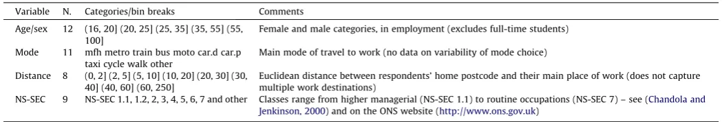
The mathematics (Fienberg, 1970) and code (Lovelace and Bal-las, 2013, Supplementary Information) used to implement IPF are described in detail elsewhere; here we illustrate in more intuitive terms how the model works.Tables 4 and 5provide samples of the raw constraint data, on aggregate and individual levels respec-tively. The spatial microsimulation model works by adjusting a large array of weights—rows corresponding to individuals and col-umns corresponding to the geographic zones under investigation— iteratively, to maximise the fit between simulated and census data. Assuming temporarily that only the four individuals represented in

Table 4were used, constraining by the distance variable inTable 5

would lead the individual with an ID of 2 to be allocated a weight of 914 for zone 1, 665 for zone 2 etc., as they are the only person who fits into that category. Clearly, many other individuals, with other characteristics would fit into the 5–10 km distance category in the entire microdataset, and this diversity is what allows the

weights to converge towards a single result for each individual-zone combination (Fig. 2).

To ensure the model is working, the simulated micro-data are aggregated and then compared with census data. Total absolute er-ror (TAE), a simple and effective goodness-of-fit metric ( William-son et al., 1998; Voas and WilliamWilliam-son, 2001), was calculated after constraining for linking variable and after each complete iter-ation (Fig. 2). Further validation tests are described in Section3.6. The weighted data provided by IPF-based spatial microsimula-tion is bulky (containing rows even for individuals who contribute very little: whose weight is close to zero) and prevents certain types of analysis. To tackle this problem, and provide a single data-set for analysis using various techniques (e.g. individual-level, geo-graphic, or agent-based methods), the ‘truncate, replicate, sample’ method of integerisation was usedLovelace and Ballas (2013). Still, the final output dataset contained 532,130 rows, representing every commuter in South Yorkshire.

3.5. Assigning work location

The spatial microsimulation model results in a large dataset containing hundreds of individuals for each zone under investiga-tion. For micro-level spatial analysis, origin–destination pairs are needed: simulated places of home and work need to be geotagged. The simplest solution to this problem is to allocate all individuals in each zone home coordinates corresponding to the zone’s popu-lation-weighted centroid. Likewise, work coordinates can be set to the nearest employment centre. This method allows for simple analyses such as the proxy for geographic isolation presented in

Fig. 3.

Rather than assuming that work centres are always located in the city centre, a more realistic approach is to acknowledge that a variety of employment centres exist, and that the relative impor-tance of each varies from place to place. This is illustrated inFig. 5,, a ward-level flow diagram of the work locations of commuters based on the outskirts of Sheffield. Although Barnsley is the closest city centre to Stocksbridge (seeFig. 3), this analysis makes it clear that Sheffield is the primary non-home workplace.

At an even finer geographical level, it is possible to discern the localities within each city and ward where people are most likely

Table 4

Sample of linking variables at the individual level (USd).

ID Age/sex Mode Distance (km) NS-SEC

1 Male, 59 Car driver 3 Lower management

2 Female, 51 Car driver 9 Higher professional

3 Male, 31 Car driver 2 Other

4 Female, 24 Walk 1 Lower management

Table 5

Sample of linking variable values for zones. The population of the most populous category is presented for each variable.

Variable) Age/sex Mode Distance (km) NS-SEC

Area code Males, 35–54 Car drivers 5–10 km Lower management

E02001509 116 1616 914 499

E02001510 94 1430 665 402

E02001511 82 1467 848 340

E02001512 152 2280 573 791

Fig. 2.Improving fit between simulated and census data across all 4 constraint variables outlined inTable 4, as illustrated by decreasing values of the total absolute error (TAE) (left) and decreases in the proportion of simulated aggregate cell values that differ from census data by more than 5% (right) after each constraint and iteration. The horizontal black lines represent 0 error and 5% of cell values, respectively.

R. Lovelace et al. / Journal of Transport Geography xxx (2013) xxx–xxx

to work based on UK census data. This is illustrated in Fig. 4. Although this level of geographic detail was not used in the final

results due to aggregation issues,13 _{it demonstrates the potential}

for highly localised work allocation based on census-derived flow data.

The analyses presented in bothFigs. 3 and 5both greatly over-simplify trip routes. The straight lines underestimate travel dis-tance, completely ignoring the transport network. A more realistic method is to randomly allocate each individual to a unique home location based on population density (or, potentially, local area classification) and estimate the route taken using shortest trip algo-rithms dependent on the mode of transport used (Fig. 6). This latter method allows for the calculation of route distances by mode, but is more complex and difficult to implement over large areas.

These methods of spatial analysis provide great insight into the meaning of aggregate statistics for groups of individuals at the city level of policy intervention. However, to gain insight into the im-pacts of schemes on individuals and local communities, agent based models may be needed. In particular, there is great potential to link the work presented here with relevant agent-based simula-tion work in the social sciences (e.g.Gilbert and Troitzsch, 2005; Gilbert, 2007) and attempts to add a geographical dimension to this work (seeWu et al., 2008).

To this endFig. 6presents the simulated route choice of the 18 commuters selected from the spatial microsimulation model, and contains both socio-demographic and geographic detail.14_The

dis-tances travelled along the transport network are clearly substantially further than represented by simple straight lines. This concept can be defined formally ascircuity, the ratio of straight-line distance to route distance (Ballou et al., 2002).Fig. 7illustrates the impact of the road network on distance travelled. Overall, the route distance represented inFig. 6is 223 km, 24% further than the straight-line distance (179 km) for the 17 commutes. As in previous studies, cir-cuity tends to decrease approximately logarithmically as a function of distance (Levinson and El-Geneidy, 2009). The spatial microsimu-lation method holds great potential for investigating the impact of

Fig. 3.Average distance to employment centre in South Yorkshire. The left-hand map illustrates how distance was calculated (using the command nncross () in the R package ‘spatstat’). The right-hand map illustrates the results—Sheffield and Rotherham are grouped together in the same travel to work zone.

Fig. 4.Employment density at the local level in Sheffield (nis the number of employees registered to each zone). These results were generated by summing all incoming flows to all of Sheffield’s 1744 Output Area (OA) administrative zones. Data provided on a CD, on request from http://www.nomisweb.co.uk/.

Fig. 5.Flow diagram illustrating popular commuter destinations for citizens of Stocksbridge. The thickness of the lines is proportional to the number of people who travel there (for reference, 661 people travel to the centre of Sheffield—illustrated by the thickest line—and 2036 people work in Stocksbridge—illustrated by the dot from which all lines radiate.n= 6338).

13_{The Output Area flow data presented in Fig. 4is difficult to work with for}

individuals allocated to specific zones, because any number between 1 and 4 is randomly set as either 0 or 3. This makes the flow data essentially probabilistic for single Output Area pairs, hence our limitation to aggregate-level analysis of this dataset here.

14_{For example, the simulated car passenger who commutes to central Sheffield in}

Fig. 6is 16 years old, is classified as class ‘other’, and lives in a family that has access to 5 cars. These, and further simulated details such as income, could, once validated, contribute towards transport interventions targeting specific commuter groups.

the travel network, especially when combined with new tools for batch-processing of shortest-route algorithms.15

3.6. Model validation

Due the dangers of using incorrect model data to inform policy, the importance of validation has been emphasised repeatedly in the spatial microsimulation literature (Clarke and Holm, 1987; Chin and Harding, 2006; Smith et al., 2009; Edwards et al., 2010; Ballas et al., 2013). Because the outputs of spatial microsimulation are by nature detailed and provided at the individual-level, valida-tion is challenging: ‘‘such detailed informavalida-tion is virtually never available at the disaggregate level for an entire region’’ ( Ravulapar-thy and Goulias, 2011, p. 37). In fact, one could argue that if indi-vidual microdata were made available at the small area level, spatial microsimulation would be obsolete.

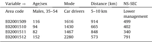
Researchers using spatial microsimulation have been innova-tive at overcoming this ‘catch 22’ situation, using a variety of meth-ods. In broad terms, there are two types of strategy available: internal and external validation (Edwards and Tanton, 2013). The first of these is relatively straightforward: the aggregated con-straint variables are compared with the aggregated results of the spatial microsimulation model for the same variables. In our mod-el, the results of this test were reassuring: the correlation between the aggregate counts from the census and those generated in our spatial microsimulation were 0.9989 overall for all 6920 data points (40 categories by 173 zones). However, the quality of the fit was better for some constraint variables than for others: the r2 _{values for the distance and mode variables were 0.9993 and}

0.9983, primarily due to the inaccuracy or our estimates of individ-uals who work mainly from home (mfh) (Fig. 8).

This internal validation result is less impressive when one con-siders that IPF always converges towards the optimal result for known constraint variables: it is the unknown cross-tabulations and target variables that we are trying to simulate with spatial microsimulation, so external should, in most cases, be the focus (Morrissey et al., 2008; Edwards and Tanton, 2013). Four methods of corroborating spatial microsimulation results with external data were identified:

Fig. 6.Simulated route choice for 20 randomly selected individuals from the spatial simulation model. Destinations were determined by (1) subsetting destination wards by distance from Stocksbridge centre, (2) assigning probabilities of working in each ward for each distance band (based on flow data presented inFig. 5) and (3) randomly selecting points within the resulting destination wards. (Workplaces of 3 people who work from home are not mapped).

Fig. 7.The circuity of the route distance as a function of the straight-line distance for 17 commuter trips modelled in Stocksbridge.

15 _{The analysis conducted one trip at a time, using the QGIS plugin ‘‘Road Path’’ for a}

simple solution with a user-friendly interface. (http://docs.qgis.org/2.0/html/en/docs/ user_manual/plugins/plugins_road_graph.html http://plugins.qgis.org/). To automate the process, Routino (http://www.routino.org/), PGRouting (http://pgrouting.org/) or the recently released R package osmar (http://cran.r-project.org/web/packages/osm) could be used. The rapid evolution of transport network data and software provides avenues for methodological advance.

R. Lovelace et al. / Journal of Transport Geography xxx (2013) xxx–xxx

Compare simulation results with real spatial microdata.16 Collect primary data from specific areas against which the

sim-ulated results can be tested.17

Compare simulation results at the aggregate level with

esti-mates from a dataset external to the model (Morrissey and O’Donoghue, 2013).

Aggregate-up the small area estimates provided by spatial

microsimulation to compare the results with real data thatis provided at higher geographies (Edwards and Clarke, 2009).

Each of these options was considered for our case study, but data constraints meant that only one, comparison of aggregate data on a target variable with a reliable external dataset, was deemed viable. The target variable chosen for this was income; Neighbourhood Statistics provides estimates of this at the MSOA level, allowing for direct comparison with our results (Fig. 9). The results show high levels of correlation (r2_{= 0.93) between simulated incomes}

and official estimates, although the spread of the values resulting from spatial microsimulation underestimated the true level of inter-zone variation in average incomes (seeTable 6).

4. Results

4.1. Aggregate-level results

Our results show that, at the aggregate level, South Yorkshire’s commuting behaviour is comparable to the national average. Nev-ertheless, the microdata illustrate inter- and intra- zone variability.

Table 7illustrates the cross-tabulations (contingency tables) that are made possible when spatial microdata are used. Univariate sta-tistics are available on mode of transport, age and number of cars but the interaction between these variables remains hidden in aggregated Census data.

Beyond illustrating the capability of spatial micrsimulation to provide estimated cross-tabulations of aggregate level data,Table 7

also provides substantive information about commuting patterns that could be applied to transport policy:

Cars dominate travel to work in South Yorkshire, to an even

greater extent than in England as a whole.

Fig. 8.Comparison of census and simulated results at the aggregate level for a selection of six categories from the mode and distance constraints. The ‘‘_20’’ category, for example, refers to the number of people travelling 10–20 km to work.

Fig. 9.Scatter graph of mean equivalised household income produced as an output from the spatial microsimulation model (yaxis) and official estimates from the Office of National Statistics for the 173 Medium Super Output Areas of South Yorkshire. (Max. and min. official estimates labelled in blue.) (For interpretation of the references to colour in this figure legend, the reader is referred to the web version of this article.)

Table 6

Contingency table illustrating the link between 2nd most common mode of TTW in an area and average values for other variables.

2nd mode N. zones Total (%) _{D(km) P car(%) D ens(People/km}2₎

MFH 18 10 17.0 68 31

Tram 4 2 10.8 53 179

Bus 95 55 11.2 54 106

Car (p) 10 6 13.5 63 40

Foot 46 27 13.2 53 112

Table 7

Summary statistics of the commuting behaviour of individuals in South Yorkshire disaggregated by mode. (Motorbike, taxi, metro and ‘other’ modes have been removed for brevity).

Mode N. % % National Age Distance (km) Ncars

Bus 31,486 7.2 7.4 38.3 7.5 0.5

Car (d) 268,496 61.1 54.6 40.1 14.3 1.9

Car (p) 38,233 8.7 5.9 33.5 14.5 1.5

Cyc 4498 1.0 2.6 38.3 5.0 1.1

MFH 45,326 10.3 9.3 40.0 0.0 1.9

Train 5709 1.3 4.6 36.9 24.6 1.2

Walk 38,406 8.7 9.7 36.6 3.1 0.8

Average – – – 39.0 11.3 1.6

16 _{Income, for example, is collected by the Census, but is not disseminated at}

aggregate levels, let alone the individual-level geocoded data required to validate the individual-level results of the spatial microsimulation model. Access to such sensitive real microdata limits the applicability of this method.

17 _{In some cases (e.g. environmental attitudes) this may be the only reliable}

validation option, as the data is simply not collected in geo-coded surveys.

The dominance of cars is even greater when measuring travel to

work in terms of distance travelled: car commuters travel on average further than all other types of commuters bar those who commute by train.

There are also substantial differences in the age profiles of

dif-ferent commuting modes: walking, which is often associate with older members of society, appears to be more prevalent amongst the young. Bicycle commuters, who are sometimes stereotyped as young (Daley and Rissel, 2011), are not much younger than than the average. Car drivers and home workers tend to be slightly older.

Car ownership, which is seldom factored-into transport policy

assessments, (Kay et al., 2011) varies with the mode of travel to work. Those who catch the bus or walk are least likely to own a car, while a those who drive to work or work from home own on average almost 2 cars per household.

4.2. Geographic variability

The results show a strong relationship between location and distance travelled. The role of location, and distance to employ-ment centres more specifically as a cause of distant commutes was explored using travel to work (TTW) zones, defined by the

Office for National Statistics at the wider regional level of Yorkshire and the Humber (Fig. 10).18_{Fig. 10shows that MSOA areas located}

in and around the conurbations surrounding Bradford, Sheffield and Hull tend to have low average commuter distances, while rural loca-tions such as the North York Moors are associated with long average commutes. This result differs from that of suburban USA (where ur-ban sprawl accounts for high commuting costs even within major conurbations), but it is hardly new or surprising (Marshall, 2008; Sexton et al., 2012). An unexpected result is the tendency of city cen-tres to be associated with high average commuter distances. This can be seen in red patches surrounded by a sea of green in the centres of Bradford, Leeds, Scarborough and Sheffield. (One hypothesis to ex-plain this is as follows: some city centres attract wealthy individuals, who tend to commute further, often by train.)

Fig. 10.Average distance travelled to work in Yorkshire and the Humber by MSOA zone. Black lines represent TTW zones.

Table 8

Contingency table of average values for continuous variables related to commuting, cross-tabulated by income bands, based on the spatial microsimulation model for South Yorkshire (n= 531,282).

Income group Proportion Age Dis (km) N.cars Income (£/yr) N.child

v.poor 10% 38 5.8 1.2 5519 0.9

poor 18% 39 8.1 1.2 10,158 1.0

below.av 22% 39 8.3 1.4 13,974 0.8

above.av 18% 39 8.9 1.6 17,902 0.6

affluent 32% 40 16.5 1.9 29,448 0.5

18 _{The wider regional level of analysis of Yorkshire and the Humber (seeFig. 1) was}

used in this case because TTW zones are large: only 3 are found in South Yorkshire (Fig. 3), so a larger area is useful to see the overall pattern. Travel to work zones are defined as ‘‘zones with a self- containment of at least 75% (which is to say that less than 25% of those who work in an area live outside it, and less than 25% of the employed residents of that area commute to workplaces outside the same area)’’ (Coombes and Openshaw, 1982).

R. Lovelace et al. / Journal of Transport Geography xxx (2013) xxx–xxx

4.3. Individual-level results

Spatial microsimulation allows one to ‘drill down’ to the indi-vidual level, target specific groups and model who (in addition to where) is most likely to benefit from specific interventions.Table 8, for example, shows simulated differences in commuting patterns between high and low income citizens in South Yorkshire as a whole.19 _{Because the individual microdata are also geocoded, we}

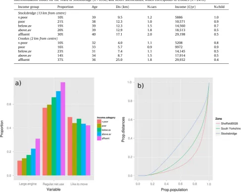
were able to conduct the same analyses for specific zones.Table 9

illustrates how the results of spatial microsimulation allow inter-and intra-zone analysis to be combined.Table 9indicates that the Sheffield028 (an MSOA zone) is more unequal in terms of income and distance travelled to work than Stocksbridge (a statistical Ward) (seeFig. 6to see their respective locations). These results, which can be compared with the regional data presented inTable 8, or re-cal-culated for smaller zones, are thus (to the extent that administrative boundaries allow) ‘frame independent’ (Horner and Murray, 2002).

To further explore differences in intra-zone inequality, com-muter work travel distances were plotted as Lorenz curves (Fig. 11b). These provide further insight into commuter patterns in each of the zones described inTable 9, and illustrate that a small proportion of the population living in Crookes accounts for a large part of the average trip distance. Stocksbridge, by contrast, has a more even distribution of commuter patterns.

Regarding the categorical target variables described inTable 3, the results imply that wealthy commuters in South Yorkshire drive larger cars, use the internet more frequently, and may be less likely to want to move than those with low incomes (Fig. 11a).

5. Discussion and conclusions

This paper has presented a spatial microsimulation approach to model commuter patterns. Whole individuals from a detailed na-tional survey were allocated to geographic zones at various levels; this provided further insight into intra-zone variability of commut-ing than is available from the use of aggregated census data alone. In addition, the careful selection of target variables not included in

Table 9

Contingency table of average values for continuous variables related to commuting, cross-tabulated by income bands, based on the spatial microsimulation model for the Ward of Stocksbridge (n= 6338) and MSOA Sheffield028, which corresponds to Crookes (n= 2470).

Income group Proportion Age Dis (km) N.cars Income (£/yr) N.child

Stocksbridge (13 km from centre)

v.poor 10% 39 9.5 1.2 5886 1.0

poor 21% 38 12.3 1.0 10,571 0.9

below.av 19% 39 12.3 1.5 14,560 0.7

above.av 20% 39 12.9 1.8 18,513 0.5

affluent 30% 40 17.1 2.0 29,198 0.5

Crookes (2 km from centre)

v.poor 10% 32 4.0 1.1 5208 0.8

poor 16% 33 5.7 0.9 9972 0.9

below.av 23% 31 7.4 1.1 14,145 0.5

above.av 14% 34 8.7 1.5 17,914 0.5

affluent 37% 36 25.0 1.8 29,932 0.4

Fig. 11.(a) Variability of vehicles (proportion of primary cars in household whose engine size is 2.0 litres or more), internet use (proportion of commuters who use the internet daily or weekly) and desire to move home depending on equivalised income. These categorical target variables are described inTable 3. (b) Lorenz curves illustrating the individual-level variability in commuter distances for 3 zones. The Gini indices associated with these curves are 0.278, 0.294 and 0.305 for Stocksbridge, South Yorkshire and Sheffield028 respectively.

19 _{The categories ‘‘very poor’’ to ‘‘affluent’’ used here are defined in (Ballas et al.,}

2005b). Statistical bins are defined as proportions of the the median income, with breaks at 50%, 75%, 100% and 125% of the median (Ballas et al., 2005b, p. 91).

the census provided insight into the relationships between com-muting behaviour and a variety of ‘target variables’ such as income, internet use, desire to move home, type of car and number of children.

From the perspective of the data-constrained policy makers mentioned in the introduction, these results are attractive: they provide a level of detail that is inaccessible for analyses based on geographically aggregated census data alone. The ability to explore the commuter behaviour of subsets of individuals based on age, distance travelled and class (constraint variables) or other variables including size of car or income (target variables) will be useful in various applications: being able to simulate the character-isticsof commuters who are most likely to benefit from certain interventions and identifyingwhere these people live and work clearly has huge potential for transport planning and policy. To illustrate the point, the distribution of low-income households reli-ant on buses can be simulated and mapped at the county level to help inform the location of new bus routes (Fig. 12). For example, if this type of analysis had been properly conducted and validated during the planning stages of the recently implemented rapid bus routes in Albuquerque mentioned in Tribby and Zandbergen (2012), the system could have been designed such that low income residents benefited from faster access to the city centre. In fact, rel-atively wealthy households (who probably have more transport options already) benefited most from the scheme (Tribby and Zandbergen, 2012). This illustrates the importance of considering not only aggregate-level impacts, but also taking into account the local and micro-level distributional effects of intervention. The spatial microsimulation approach to modelling commuter patterns outlined in this paper provides a foundation for investigating such effects. In addition, we have demonstrated how spatial microsim-ulation methods can enrich transport models with policy relevant socio-economic variables at individual and small-area levels. In

broader terms, we hope this paper promotes a closer collaboration between the fields of transport modelling, spatial microsimulation and spatial microsimulation.

Another possibility opened-up by the inclusion of the individual level data (but not explored in this paper) is more detailed energy analysis: previous studies have tended to focus on energy use in transport at national or city scales of (Lovelace et al., 2011; Wood-cock et al., 2007), omitting important information about its social distribution (seePreston et al., 2013for a UK example).

Despite these enticing possibilities, is important to remember that the results aresimulated. Consequently, we must distinguish between linking variables (or constraint variables)—these are con-strained by known census aggregates and are therefore trustwor-thy—and target variables which are more tentative estimates based on correlations between target and linking variables at the national level. As noted in Section3.1, target variable estimates rely on an often unstated assumption: that the relationships be-tween variables at the national level (e.g. bebe-tween distance trav-elled to work and income) tend to remain at local levels. This assumption cannot be expected to hold everywhere, so results aris-ing from target variables are expected to underplay the true level of spatial variability. Where possible, target variable results should be corroborated against independent datasets (Edwards and Clarke, 2009).

Many transport interventions have wide-ranging impacts on commuters. These depend on geographical and individual-level factors, and the importance of the latter especially is often over-looked in transport policy (e.g. Tribby and Zandbergen, 2012). The micro-level methods presented in this paper therefore have great potential, to enable researchers and transport planners to better model and predict the impacts arising from various inter-ventions. With the current focus on energy and sustainability in transport (Chapman, 2007), there is a risk that distributional

Fig. 12.Proportion of population who is earning less than 50% of South Yorkshire’s median incomeandlives in a car free household within the 173 MSOA boundaries of the metropolitan county, according to the spatial microsimulation model. Translucent red dots represent bus stops (data from http://data.gov.uk/dataset/nptdr).

R. Lovelace et al. / Journal of Transport Geography xxx (2013) xxx–xxx