White Rose Research Online
[email protected]
Universities of Leeds, Sheffield and York
http://eprints.whiterose.ac.uk/
This is an author produced version of a paper published in Intelligent Systems
Reference Library.
White Rose Research Online URL for this paper:
http://eprints.whiterose.ac.uk/77251/
Paper:
Malleson, N, Evans, A, Heppenstall, A and See, L (2014)
Optimising an
Agent-Based Model to Explore the Behaviour of Simulated Burglars.
Intelligent Systems
Reference Library, 52. 179 – 204.
the Behaviour of Simulated Burglars
1Nick Malleson, 2,3Linda See, 1Andrew Evans and 1Alison Heppenstall
1School of Geography, University of Leeds, Leeds, UK
2International Institute of Applied Systems Analysis, Laxenburg, Austria
3Centre for Applied Spatial Analysis, University College London (UCL), London, UK
Abstract Agent-based methods are one approach for modelling complex social systems but one issue with these models is the large number of parameters that re-quire estimation. This chapter examines the effect of using a genetic algorithm (GA) for the parameter estimation of an agent-based model (ABM) of burglary. One of the main issues encountered in the implementation was the computation time required to run the algorithm. Nevertheless a set of preliminary results were obtained, which indicated that visibility is the most important parameter in the de-cision of whether to burgle a house while accessibility was the least important. Such tools may eventually provide the means to gain a greater understanding of the factors that determine criminological behaviour.
http://dx.doi.org/10.1007/978-3-642-39149-1_12
1 Introduction
make assessments of their situation over time (or during each iteration of the mod-el) and then make decisions in response to these assessments (Bonabeau, 2002). By providing realistic environments and rules that are based on observed and ex-pected patterns of human behaviour, it is possible to create models that can simu-late real world systems (Moss and Edmonds, 2005).
Classic examples of ABMs are the Sugarscape model of Epstein and Axtell (1996), which simulates wealth accumulation through sugar harvesting in a simple environment, and Schelling’s (1971) model of segregation, which has been simu-lated by a number of researchers in the past using an ABM approach (see e.g. Omer, 2005 and Crooks, 2008). ABMs are now being applied in a variety of dif-ferent domains, e.g. ecology (Grimm and Railsback, 2005), economics (Tesfatsion and Judd, 2006) and more recently, criminology (Malleson 2009; 2010a, b, c).
Although ABMs represent a way to capture complexity in social systems, they have issues related to parsimony, i.e. they contain a potentially large number of parameters. Some parameters can be determined through expert knowledge or can be derived from field measurements or social surveys. However, many others are unknown and therefore require a method to determine their values. The need to calibrate a model is not limited to ABMs and many different methods of search and optimisation are available. However, classical search methods are not effec-tive in finding large numbers of parameters so other methods such as genetic algo-rithms (GAs) are needed.
which parameters varied considerably between runs and therefore had little effect on the overall results of the simulations.
More recently, Stonedahl (2011) undertook a comprehensive evaluation of GAs for parameter estimation of ABMs in a number of applied areas including ar-chaeology and viral marketing, which showed that GAs can be effective tools for uncovering and further investigating interesting behaviours in these applied areas. However, the research also recommended experimentation with further applica-tions as well as a consideration of multi-objective optimisation problems. The aim of this chapter is to provide an example of single-objective GA parameter estima-tion in another applicaestima-tion area, i.e. crime. An ABM of burglary, which has been previously developed and applied to the city of Leeds in the United Kingdom (Malleson et al., 2010a, b, c), is used to examine the use of a GA for parameter es-timation. The chapter begins with on overview of basic crime theory and previous modelling research, including why ABMs are well suited to modelling criminal behaviour. This is followed by a brief overview of optimisation methods and the basic mechanism of a GA. The ABM of burglary is then described including the parameters to be optimised and the GA experimental settings. This is followed by the results of some preliminary experiments and initial reflections upon this meth-od for parameter estimation. The chapter concludes with plans for further research in this area.
2 Theoretical Background
Individual acquisitive crimes are the result of the convergence of a huge number of factors. These include, but are not limited to:
• The motivation of the offender;
• The behaviour of other people including the victim(s); • The influence of the surrounding physical environment; • Wider social factors such as levels of community cohesion.
how comfortable an offender feels in a particular area (i.e. whether or not they stand out) as well as broader effects that influence where people travel to within a city.
Although the system is clearly complex in the scientific sense of the word, oc-currences of crime are not random. Crime patterns can remain stable over long pe-riods of time and a large body of literature has evolved to explain them. This sec-tion will outline some of the most relevant criminological findings which form the basis of ABMs of crime as introduced in section 3. As well as demonstrating that the model closely reflects the reality of the real-world crime system, it will make clear why the ability of agent-based modelling to account for the behaviour and interactions of numerous individuals makes it the most suitable methodology for modelling acquisitive crime and burglary in particular.
2.1 The Spatial Scale of Crime Analysis
2.2 Environmental Criminology Theories
The movement in crime research towards using individual-level geographies also resonates with the major theories in Environmental Criminology. As this section will illustrate, these theories focus specifically on the spatio-temporal behaviour of the individual(s) involved in crime events and the intricacies of the immediate sur-rounding physical environment.
Routine activity theory (Cohen and Felson, 1979) explores the interactions be-tween victims, offenders and other people who might influence an individual crime event (e.g. passers-by, police, etc.). For the crime to occur, the theory stipu-lates that an offender must meet a victim at a time and place with an absence of others who might prevent the crime. This convergence depends on the routine ac-tivities of the people involved. For example, a burglar might come into contact with a vulnerable house (the potential victim), but might not be able to commis-sion a crime if the routine activities of the residents or neighbours mean that they are in the area at the same time and will notice a crime taking place.
The geometric theory of crime (Brantingham and Brantingham, 1981) shares many similarities with routine activities theory, but focuses more explicitly on the interdependencies between a person’s knowledge of the environment, i.e. their
awareness space, and criminal opportunities. The theory considers how the routes used to travel around a city influence a person’s awareness space and hence the spatio-temporal locations in which offenders are likely to commit a crime. Bur-glars do not search for targets at random; instead they are likely to search near im-portant ‘nodes’ such as friends’ houses, schools, work places, or places of leisure (Brantingham and Brantingham, 1993). Thus house vulnerability to burglary is less relevant if the house itself is not within the awareness space of a person who might attempt to burgle it.
The final theory that the model logic attempts to replicate is the rational choice perspective (Clarke and Cornish, 1985). This suggests that the offender’s decision to offend is a cost-benefit analysis weighing up potential rewards of a successful crime with the risks of being apprehended. Thus a crime will only be committed if it is perceived as profitable. It is important to view the concept of rationality as ‘bounded’, such that a decision that might appear to be optimal to one person (in a specific situation with their own thoughts and motivations) might be blindingly ir-rational to another.
emphasis is on the individual-level nature of crime occurrences. The crime system is driven by the behaviour and interactions of individual people situated in a high-ly detailed local environment. Aggregating such a system (either spatialhigh-ly or tem-porally) will hide important lower-level dynamics that ultimately explain why crime takes place in the places that it does.
2.3 Traditional Crime Models
Traditionally, quantitative crime models have used area-based crime data in re-gression style modelling (see e.g Brantingham and Brantingham, 1998). Kongmuang (2006) provides a comprehensive review of the methods employed, where a number of common characteristics can be identified. For example, model accuracy is usually estimated through the Akaike Information Criterion (AIC) or a goodness-of-fit statistic such as R2. Other drawbacks are outlined below although
we do recognise that there are also many advantages of statistical methods which are not discussed further in this chapter.
Firstly, statistical models generally utilise simple functional relationships, e.g. they cannot adequately capture the evolution of individuals through time and the effect this has on their behaviour. In contrast, ABMs can represent these complex real world interactions including the intricate personal trajectories and histories of individuals. Statistical techniques generally aim to reduce variables to enhance explanation at a cost to predictive power, so cannot account for the complexity of the environmental backcloth and the non-linear human or human-environment interactions that drive the system.
Secondly, the use of spatially aggregated data -- to represent crimes, de-mographics, the environment, etc. -- hides important lower-level relationships be-tween crime, individuals and the environment. Similarly, it is not possible to cap-ture important feacap-tures of the physical environment such as accurate travel times, impassable barriers or road-network layout unless individual environment objects (roads, buildings, parks, etc.) are accounted for explicitly.
In general, the dynamics that drive the crime system (as with other social sys-tems) are not captured directly in aggregate models. This makes it difficult both to explore criminology theory -- which inherently focuses on the spatio-temporal be-haviour of individual people -- and to make crime forecasts at the same time. ABMs, however, provide an alternative approach by allowing these individual en-tities to be modelled directly. In this manner, it is possible to capture the true rich-ness of the system and much more closely reflect an individual’s unique circum-stances and behavioural characteristics.
3 Agent-Based Models (ABMs) of Crime
ABMs have a number of clear advantages over other modelling and analysis tech-niques when it comes to understanding crime. Crime tends to be the result of indi-viduals acting on the basis of their history and current environment, either alone or in collaboration. ABMs, unlike other techniques, take as their starting point unique individuals (‘agents’) with their own history and decision making capacities, and these individuals are placed in a complicated environment to discover the resultant behaviour. As in a real crime system, agents will both respond to and adjust the current environment (e.g. agents may cause an area’s attractiveness to housebuy-ers to fall). The agents in ABMs can interact and collaborate in group behaviour and decision making. However, there is also no reason why larger, aggregate groupings and decision making (e.g. government policy groups) cannot also be represented and respond to the system. In short, ABMs represent social systems in the way we intuitively understand social systems ourselves.
mi-crosimulations that look at the results of such interactions, after multiple events and with low populations, these techniques become problematic. With ABM, in-dividuals carry their history with them, either implicitly or explicitly, and this his-tory can be analysed to see how it affects their decision making. Finally, ABMs can represent a wide range of environments, from the very abstract, to the ex-tremely realistic. This allows us to explore and understand the effects of the envi-ronment on behaviour at a very detailed level. For example, it is possible to look at the effect that a specific change in a public transport route might have on crimi-nal opportunity. Moreover, once an ABM is set up, a wide variety of different analyses and scenarios can be run without adjusting the underlying model, unlike many other techniques, where the model must be specifically designed from the ground up to answer a single research question.
Given these advantages, it is somewhat surprising how slowly the development of ABM of crime has progressed. Nevertheless, the last ten years or so has seen an increased interest in the technique, and a number of groups are building ABMs of crime of various levels of detail. In general, most current ABMs of crime attempt to replicate the major components of the criminal system to some degree: offender motivation and decision-making, offender behaviour and movements, victimhood and guardianship. However, given the complexity of the system, it should come as no surprise that most concentrate on building realism in one of these components rather than all of them. In addition, the realism of the environment within the model varies a great deal, not least because of the broad division in agent-based modellers between those who believe ABM should be utilised as abstract ‘thought experiments’ to explore key theoretical behaviours and ideas, and those who be-lieve that it is possible to build a more detailed model of the real world for explo-ration and prediction (see, for example, Di Paolo et al., 2000, for arguments for the former).
Malleson et al. (in press) give a full review of ABMs used to model crimes that have a predictable geographical component (that is, crimes like burglary and street theft, as opposed to crimes like domestic violence and fraud, on which geog-raphy have less obvious effects). However, notable models at the more abstract end of the scale include Winoto (2003); van Baal (2004); Brantingham and Bran-tingham (2004; BranBran-tingham et al. 2005a;b; 2008); Dray et al. (2008a), and Wang
organisa-tion, e.g. gang crime and civil violence (Lustick 2006; Huddleston et al. 2008; Bhavnani et al. 2008; Cherif et al. 2009; Egesdal et al. 2010). Some of the ethical issues facing agent-based modellers of crime are explored by Evans (2012).
4 Optimisation of Complex Models
We now consider the specific issue of parameter estimation in ABMs using meth-ods of optimisation, which are techniques that search a problem space for the best solution possible given the complexity of the problem, the computational re-sources available and the objectives or constraints of the problem (Goldberg, 1989). Mathematically this involves finding what are referred to as a set of deci-sion variables that minimise or maximise one or more objective functions (i.e. a function specific to the problem which determines how good the solution is) sub-ject to satisfying a set of constraints. For example, the decision variables may be the quantity of material that flows between a set of different distribution points where the objectives are to minimise the distance travelled while maximising the profit subject to certain routes not being allowed due to direction of flow or exces-sive gradients. Some problems may have a single optimal solution where the main challenge is finding the global optimum in a solution space characterised by mul-tiple local minima (or maxima depending upon the way the problem is formulated) without having to fully search the whole parameter space. In contrast, in more complex problems or in those with multiple objectives, there is no single solution that simultaneously optimises all conflicting objectives. The result is a set of alter-native optimal or feasible solutions of similar fitness that represent trade-offs be-tween the different objectives. Optimisation provides the mechanism to find this set of solutions, which are called Pareto optimal solutions. Other methods, such as multi-criteria decision making, are then needed to further evaluate the solutions that are identified during the optimisation process. Many real world problems are characterised by the need to take conflicting multiple objectives into account. In hydrology, for example, multi-objective optimisation methods are used extensive-ly for calibrating physical and conceptual hydrological models (Yapo et al., 1998; Vrugt et al., 2003; Efstratiadis and Koutsoyiannis, 2009).
algo-rithm; and run the algorithm to obtain the results (Deb, 2001).The next section deals specifically with step 6, i.e. different methods of optimisation.
4.1 Methods of Optimisation
A number of different optimisation methods have been developed in the past to handle problems involving single and multiple objectives. Classical (or conven-tional) optimisation methods were developed using differential calculus. They in-volve finding an analytical solution on functions that are continuous and differen-tiable, e.g. the simplex method (Maros and Mitra, 1996). These are referred to as strong methods and are deterministic. On the other end of the spectrum are weak classical methods, which involve a random or stratified random sampling of the search space in order to find the solution, which are inefficient methods. These classical methods have a number of disadvantages (Goldberg, 1989; Deb, 2001). For example, the convergence of an optimal solution depends upon the initial so-lution and they are not efficient for problems with discrete rather than continuous search spaces. Moreover, they are not efficient in solving non-linear, complex problems with large search spaces and many conflicting objectives and they can-not be parallelized efficiently since they use a single search path to obtain the op-timal solution. For this reason, a set of intermediate methods have been developed that contain a stochastic element and which use more effective search strategies to avoid being trapped in local minima, e.g. simulated annealing, tabu search and evolutionary methods such as genetic algorithms (GAs). The focus of this research is on GAs, which are described in more detail in the sections that follow.
4.2 Genetic Algorithms (GAs)
number of individuals, a much larger group is being evaluated implicitly. By this mechanism, a GA can ‘home in’ on the space with the highest-fitness individuals. This combination of parallelism, along with the other major components of a GA which produce the evolution of fitter solutions, i.e. selection, mutation and crosso-ver, make this approach a very powerful and efficient tool.
[image:12.595.134.460.362.515.2]GAs follow the same basic set of steps as outlined in Figure 1. A population is first initialised and the objective functions are then set. The fitness of each indi-vidual is assessed and on the basis of this, the fittest in the population are selected for reproduction via crossover. This continues over many generations or iterations until predefined criteria are satisfied, e.g. a certain threshold value for the objec-tive function has been reached. For a more detailed overviews of GAs, the reader is referred to Goldberg (1989), Davis (1991), Michalewicz (1992), Bäck and Schwefel (1993) and Eiben and Smith (2003). For an overview of GAs in the con-text of geographical optimisation, Xiao (2008) provides an excellent introduction.
Fig. 1. The basic operation of a GA (adapted from Weise, 2009).
The following sections will briefly outline the main generic parameters and pro-cesses that all GAs share.
4.2.1 Initial population
method is that the GA starts with a set of approximately known solutions and therefore may converge to an optimal solution faster than the first method. The disadvantage is that genetic diversity may be restricted and limit the ability of the GA to generate optimal solutions that might only be arrived at through a random starting position.
4.2.2 Representation
Most of the problems suitable for GAs involve identification of a set of parameters that need to be represented in such a way as to allow evolutionary operators to be effectively applied. As GAs are robust, there is little need to rigorously identify the ‘best’ representation for a particular problem (Goldberg, 1989). There are two broad methods that can be used for representation: binary alphabets (Holland, 1975) and real numbers (Davis, 1991; Beasley et al., 1993; Michalewicz and Jani-kow, 1991; Michaelewicz, 1992). There is no single ‘correct’ coding method for encoding a problem; the mode of representation is dependent on the problem. However, the coding sequence must adequately represent the problem to ensure that the optimal solution is available to the algorithm and be bounded by an allow-able range for the parameters.
4.2.3 Fitness and Selection
In order to evolve better performing solutions, the fittest members of the popula-tion are selected and randomly exposed to mutapopula-tion and recombinapopula-tion (as de-scribed below). This produces offspring for the next generation. The least fit solu-tions die out through natural selection as they are replaced by new recombined, fitter, individuals. Evaluation of the fitness of the individuals involves some form of comparison between observed and model data, or a test to see if a particular so-lution meets pre-defined criteria or constraints. In this work, the Standardised Root Mean Square Error (SRMSE - Knudsen and Fotheringham, 1986) is used to estimate the difference between real crime data and the model results.
Table 1. Description of several of the most common forms of parental selection
Selection Type
Description
Ranking The population is sorted from best to worst. The number of copies that an indi-vidual receives is given by an assignment function and is proportional to the rank assignment of an individual.
Tournament A random number of individuals are selected from the population. The best in-dividual from this group is chosen as a parent for the next generation. This pro-cess is repeated until the mating pool is filled.
Roulette
Wheel Individuals are mapped to contiguous segments of a line, such that each indi-vidual’s segment is equal in size to its fitness. A random number is generated and the individual whose segment spans the random number is selected. This process is repeated until the desired number of individuals is obtained.
Truncation Truncation sorts individuals according to their fitness (from best to worst). Only the best individuals are selected to be parents.
4.2.4 Selection pressure
Along with the selection method, the selective pressure parameter is critical. This parameter measures the probability of the best individual being selected compared to the average probability of selection and drives the algorithm towards a solution. The value for this parameter should be carefully selected as too much selective pressure can lower the diversity within the population resulting in sub-optimal so-lutions. Conversely if the selection pressure is too low, the population remains too diverse and the optimal solution is not found.
4.2.5 Recombination/Crossover
Fig. 2. Representation of recombination between two parents to produce an offspring
There are several methods of recombination available; the suitability of the method is dependent on the types of genes or variables stored in the chromosome. The three most common approaches are intermediate, line and extended line re-combination methods. In intermediate rere-combination, the variable values of the offspring are randomly chosen from between the values of the parents. Normally values of up to 25% outside this range can be used, which has been chosen to en-sure that statistically a space covered by the recombination does not decrease in size with time leading to a loss in diversity. The position of the variable chosen on the line determines how much each parent contributes to the offspring and is cho-sen uniformly at random for each gene. Line recombination is similar to interme-diate recombination except that the same random number is used for selecting the value of every gene in a chromosome. Extended line recombination is different from the above techniques in that the variable range is not limited to a range around the parents. The probability of any particular value being taken is not uni-form but varies with a high probability near the parents and a low probability far away from the parents. The probability distribution can also be chosen to favour the fitter parent. The value controlling the amount of the parent that is used is gen-erated randomly and then used for selecting the value of subsequent genes.
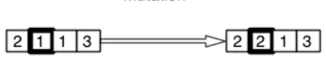
4.2.6 Mutation
Fig. 3. Illustrating the mechanism of mutation
The literature offers no strict guidelines for the selection of the size of the mu-tation step. The optimal step-size depends on the research problem and may even vary during the optimisation process. Small mutation steps are acknowledged in the literature as being successful, especially when the individual is already well adapted. However, large mutation steps can, when successful, produce good re-sults very quickly. A good mutation operator should therefore produce small step-sizes with a high probability and large step-step-sizes with a low probability.
In the next section, the ABM burglary model is introduced along with the set-tings of the GA for parameter estimation.
5 The Agent-Based Burglary Model
5.1 Purpose of the Model
The motivation behind the model is to simulate the spatio-temporal locations of burglaries at the city scale and, ultimately, to provide a framework for modelling and testing our understanding of the criminal system. The model runs for a fixed length of simulated time -- sufficient to reach dynamic equilibrium -- so does not predict the actual number of crimes. Instead, we focus here on the values of the behavioural parameters that drive the behaviour of the agents to determine what these tell us about the behaviour of burglars in the real world.
There is no notion of the processes that lead to someone ‘becoming’ a burglar; each agent has only one purpose which is to commit burglary. In addition, there is no notion of punishment or capture – offenders are not removed from the system, nor are their drivers adjusted by any kind of punishment. Although variables such as community guardianship help to determine whether a property is chosen for a crime, a chosen target is always successfully victimised. There is also no commu-nication between agents; all offenders are currently lone individuals without a shared understanding.
The model generates a spatial distribution of crimes, taking into account a va-riety of offender behaviours, environmental factors, and victim and guardian at-tributes.
5.2 Data and the Study Area
The study area for this research covers 1,700 hectares in the city of Leeds, UK. The area contains some of the most deprived neighbourhoods in the country and was earmarked for an ambitious urban renewal scheme which makes it an ideal candidate for predictive crime modelling. Figure 4 illustrates the data used to rep-resent the study area in the simulation.
• Communities are generated using the Output Area geography (a census area
boundary containing approximately 100 houses) and classified using the Output Area Classification (OAC: Vickers and Rees, 2007). This allows community types to be compared quantitatively.
• The home locations of offenders were estimated from police recorded crime
• Roads and buildings are established from Ordnance Survey MasterMap data
(the Integrated Transport Network and Topographic Area data sets respective-ly)
• Expected data are required to validate the model. The data used here are the
[image:18.595.136.507.275.542.2]number of burglaries per Output Area that occurred in 2001. This year was chosen because it corresponds closely with the timing of the UK census from which community demographics are estimated. As mentioned in section 4.2.3, the SRMSE is used to compare model results to expected data at the output ar-ea level.
Fig. 4. Datasets used in the ABM of burglary
5.3 State Variables and Scales
5.3.1 The Agents
The model is comprised of agents representing offenders. Victims and guardians are represented through environmental variables, e.g. the estimated level of com-munity cohesion. Each offender agent is assigned a home building (and associated community) at model initialisation. This location, derived from real offender data, is where the agent lives. The main agent variable, which changes during the model run, is the burglary motive. This variable increases over time and determines whether or not a burglar will choose to target an individual house; more details follow in section 5.3.3. Once a burglary has been committed, this level falls to ze-ro.
5.3.2 The Environment
Objects within the environment build up a substrate in which the agents act. There are three types of objects:
• Roads are used to restrict the possible spatial locations of the agents. In the full
version of the model, roads can be used to simulate different transport speeds and routes (e.g. a car driver moving faster along a major road) but in this sim-plified version all agents move at a constant speed of 4 miles per hour (a fast walking pace).
• Buildings represent the houses in which agents live and also represent the
po-tential victims of burglary. Their spatial locations and attributes have been es-tablished from the Ordnance Survey MasterMap geographic data product.
• Communities represent the neighbourhoods in which the houses are located.
They will influence whether or not a burglar chooses a particular house and al-so determine where an offender starts their search.
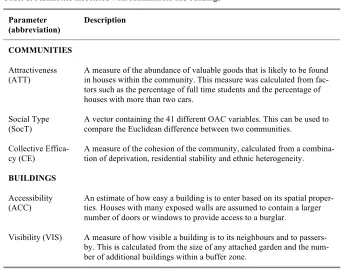
Table 2. Parameters associated with communities and buildings
Parameter (abbreviation)
Description
COMMUNITIES
Attractiveness (ATT)
A measure of the abundance of valuable goods that is likely to be found in houses within the community. This measure was calculated from fac-tors such as the percentage of full time students and the percentage of houses with more than two cars.
Social Type (SocT)
A vector containing the 41 different OAC variables. This can be used to compare the Euclidean difference between two communities.
Collective Effica-cy (CE)
A measure of the cohesion of the community, calculated from a combina-tion of deprivacombina-tion, residential stability and ethnic heterogeneity.
BUILDINGS
Accessibility (ACC)
An estimate of how easy a building is to enter based on its spatial proper-ties. Houses with many exposed walls are assumed to contain a larger number of doors or windows to provide access to a burglar.
Visibility (VIS) A measure of how visible a building is to its neighbours and to passers-by. This is calculated from the size of any attached garden and the num-ber of additional buildings within a buffer zone.
5.3.3 Process Overview and Scheduling
The model is initialised with data that allocates offenders to households, attributes to buildings and transport components, and initialises the state variables of the of-fenders. Offenders start with nothing in their awareness space. At each time step, all offenders decide on actions determined by their internal states. The sequence of offenders is random.
1. At 09:00 simulated time, the agent chooses a community to travel to in search of a burglary target. The following formula is used to assign the likelihood, L, of choosing each community, a, relative to their current location, c, and their home community, h:
L = w1*(1/dist(c,a)) + w2*Attract(h,a) + w3*SocialDiff(h,a) (1) + w4*PrevSucc(a)
where dist(c,a) represents the distance (travel time) from their current location to the target community, Attract(h,a) represents the relative attractiveness of the community compared to the agent’s home area, SocialDiff(h,a) returns the simi-larity of the target community and the agent’s home (where similar communities are favourable) and PrevSucc(a) returns the number of times an agent has had a successful burglary in the past. Importantly, the weights w1 to w4 can be used to assign an importance to each factor -- if a weight is large then the parameter will have a greater influence on the agent’s behaviour. Roulette-wheel-selection is used to randomly choose a community from all of those available such that those with a greater likelihood value have a greater chance of being chosen.
2. On the way to their destination, the agent observes each house that they pass and a ‘risk’ for burglary is calculated as follows:
R = (w5 * CE + w6*ACC + w7*VIS) / (w5 + w6 + w7) (2) where CE is the perceived collective efficacy of the surrounding area, ACC repre-sents the accessibility of the target building (how easy it is to enter) and VIS repre-sents the visibility of the building to neighbours and passers-by (where high visi-bility increases the risks). If this risk value is lower than the agent’s current burglary motive, then the agent might commit a burglary - the probability of actu-ally committing a burglary increases exponentiactu-ally as the difference between risk and motive increases. Again, weights applied to each parameter determine how much of an influence each factor will have over the agent’s decision.
If the burglary is successful, then the agent travels home. In this manner the model has been configured to allow for a variation in offending behaviour (the same agent will not always choose the same house) but agents will, on average, always commit one burglary per day.
6 Exploring the Dynamics of Criminal Behaviour
The model outlined in section 5 is an advanced ABM that attempts to closely rep-resent criminological theory and the experiences of crime-reduction experts in the field. There are 7 different variables that determine where burglar agents will start searching for targets and which houses, in particular, they will actually victimise. Although some experimentation with changing the parameters can be undertaken manually through trial-and-error, the number of combinations that can be tested, even with 7 parameters, is limited. Thus, the GA provides a more comprehensive approach to more intelligently explore the entire 7-dimension parameter space. This can help to determine which parameters have the most substantial influence on the model, and the values may eventually inform our understanding of the be-haviour of burglars in the real world.
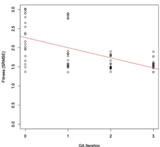
A set of preliminary experiments have been undertaken here using a GA to find the values of the 7 parameters. A population of 20 individuals was used and the GA was tracked over three iterations. The fitness of each model configuration (or ‘chromosome’) is provided in Figure 5, which is plotted against the iteration number. As would be expected, the GA is able to identify which model configura-tions result in the lowest error and, hence, which should be used to generate the configurations in the next iteration. Accordingly the model error decreases with each subsequent iteration. Figure 5 also highlights some clustering of fitness val-ues after the initial (random) population undergoes an evolution. This illustrates that the algorithm is fine-tuning the ABM in different parts of the parameter space that have the lowest error.
Fig. 5. Fitness of all the chromosomes by GA iteration
Table 3. Values of the parameters after each iteration
Iteration Fitness w1 w2 w3 w4 w5 w6 w7
0 1.372 0.719 0.668 0.736 0.683 0.541 0.291 0.984
1 1.362 0.719 0.668 0.736 0.683 0.541 0.291 0.984
2 1.372 0.719 0.668 0.736 0.683 0.541 0.291 0.984
3 1.365 0.689 0.717 0.781 0.727 0.510 0.241 1.000
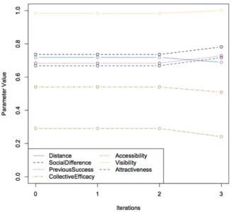
[image:23.595.128.466.522.623.2]Figure 6 illustrates the change in parameter value for these best models. Inter-estingly, the Visibility parameter is consistently assigned a high value, which im-plies it is an important factor in the agent’s decision compared to other variables. Conversely, Accessibility appears to have only a marginal importance. Explana-tions for these findings will be discussed in the following section.
Fig. 6. Parameter values for the best model after each GA iteration
picture of the underlying point patterns and is commonly used by police analysts (Chainey and Ratcliffe, 2005).
Fig. 7. Results from the three best model iterations after 1, 2 and 3 iterations
differences in configuration, which suggests that small changes to any of the agents’ behavioural parameters have little effect on the model results. Some small differences can be seen in the centre of the study area where some small hotspots are picked up differentially between the three models. Any discrepancies are likely to be a result of the probabilistic nature of the model (recall that with sufficient computing power each model would have been run a large number of times to cal-culate an average error value) although there would be scope to investigate what might be generating these differences, e.g. the slight decrease in the distance, col-lective efficacy and accessibility parameters in ‘Model 3’ and a slight increase in all the others. However, it is encouraging that small parameter changes have little effect on the model results because, were this not the case, it would be more diffi-cult to be confident in the robustness of the results. This represents another con-siderable advantage of the application of an optimisation algorithm to this model.
7 Discussion and Conclusions
This paper presented some very preliminary attempts at using a GA to estimate the parameters of an ABM of burglary. These initial findings indicated that the weight associated with the visibility parameter was consistently high. This means that with the models that closely matched the observed crime data, the agents were more likely to burgle houses that were well hidden from their neighbours and passersby. In the ABM used here, this feature was estimated by combining the physical size of a house’s garden with a measure of its isolation (i.e. the number of other properties in the immediate surrounding area). Conversely, the accessibility parameter was consistently the least important. This parameter is calculated by es-timating the number of exposed walls in each building such that detached houses are at a greater risk of being burgled than semi-detached houses or terraces be-cause there are likely to be a larger number of entry points. Why this building fea-ture appears to be less important, however, is less clear. One of the next steps will be to explore these geographical parameters is more detail.
hardware, each GA iteration -- with a population of only 20 chromosomes -- re-quired approximately 20 hours to complete. An associated side effect of the com-putation time is that it is not feasible to run each individual model configuration multiple times, which would be preferable because it would give a more compre-hensive assessment of the model error (the simulation is probabilistic so each run will lead to slightly different results). Future work will port the model to more powerful computer systems and run a GA with a larger population for a larger number of iterations and with multiple runs per model configuration. Only then will it be possible to more exhaustively examine the behaviour of the parameters in relation to burglar behaviour in a real-world setting.
The implications of using such an approach when scaling up an ABM to a much larger area, with larger numbers of individuals and with a much larger num-ber of parameters is clearly evident from these preliminary experiments. Ambi-tious ABM projects such as modelling the entire economy of the United States (Farmer and Foley, 2009) will clearly face major computational challenges in the future. But without methods like GAs, the task of parameter estimation would render such modelling approaches infeasible.
References
Andresen, M., & Malleson, N. (2011). Testing the Stability of Crime Patterns: Implications for Theory and Policy. Journal of Research in Crime and Delinquency, 48(1), 58–82.
van Baal, P (2004). Computer Simulations of Criminal Deterrence: From Public Policy to Local Interaction to Individual Behaviour. Den Haag, The Netherlands: Boom Juridische Uitgevers. Bäck, T. & Schwefel, H.-P. (1993) An Overview of Evolutionary Algorithms for Parameter
Op-timization. Evolutionary Computation, 1(1), 1-23.
Beasley, D., Bull, D.R. & Martin, R.R. (1993). An Overview of Genetic Algortihms: Part 1, Fundamentals. University Computing, 15(2) 58-69.
Bhavnani, R., Miodownik, D., and Nart, J. (2008) REsCape: an Agent-Based Framework for Modeling Resources, Ethnicity, and Conflict. Journal of Artificial Societies and Social Simu-lation 11 (2), 7 [Online]. Retrieved on 16 June 2011 from:
http://jasss.soc.surrey.ac.uk/11/2/7.html
Birks, D. (2005). Computational criminology: A multi-agent simulation of volume crime activi-ty. Presentation to the British Society of Criminology Conference, University of Leeds, UK. Birks, D. (2007). Synthesis over analysis: using agent-based models to examine the interactions
of crime. Presentation at the Fifth National Crime Mapping Conference, London.
Birks, D. J., Donkin, S., and Wellsmith, M. (2008). Synthesis over analysis: Towards an ontolo-gy for volume crime simulation. In Liu, L. and Eck, J., editors, Artificial Crime Analysis Sys-tems: Using Computer Simulations and Geographic Information Systems, pp 160–192, Her-shey, PA. Information Science Reference
Birks, D., Townsley, M., & Stewart, A. (2012). Generative Explanations of Crime: Using Simu-lation to Test Criminological Theory. Criminology, 50(1), 221–254.
Brantingham, P. J., & Brantingham, P. L. (1981). Notes on the geometry of crime. In P. J. Bran-tingham & P. L. BranBran-tingham (Eds.), Environmental criminology (pp. 27–54). Prospect Heights.
Brantingham, P. L., & Brantingham, P. J. (1993). Nodes, paths and edges: Considerations on the complexity of crime and the physical environment. Journal of Environmental Psychology, 13(1), 3–28.
Brantingham, P. L. and P. J. Brantingham (1998). Mapping crime for analytic purposes: Loca-tion quotients, counts, and rates. In D. Weisburd and T. McEwen (Eds.), Crime Mapping and Crime Prevention, Volume 8 of Crime Prevention Studies, pp. 263–288. Monsey, NY: Crim-inal Justice Press.
Brantingham, P. L. and Brantingham, P. J. (2004). Computer simulation as a tool for environ-mental criminologists. Security Journal 17(1), pp. 21–30.
Brantingham, P. L., Glasser, U., Kinney, B., Singh, K., and Vajihollahi, M. (2005a). A computa-tional model for simulating spatial aspects of crime in urban environments. Proceedings of the 2005 IEEE International Conference on Systems, Man and Cybernetics 4, pp. 3667–3674. Brantingham, P. L., Glasser, U., Kinney, B., Singh, K., and Vajihollahi, M. (2005b). Modeling
urban crime patterns: Viewing multi-agent systems as abstract state machines. Proceedings of the 12th International Workshop on Abstract State Machines, pp. 101–117, Paris.
Brantingham, P. L., Glasser, U., Jackson, P., Kinney, B., and Vajihollahi, M. (2008). Master-mind: Computational modeling and simulation of spatiotemporal aspects of crime in urban environments. In Liu, L. and Eck, J., editors, Artificial Crime Analysis Systems: Using Com-puter Simulations and Geographic Information Systems, chapter 13, pp. 252–280. IGI Global. Chainey, S., & Ratcliffe, J. (2005). GIS and Crime Mapping (1st ed.). Chichester: John Wiley
and Sons.
Cherif, A., Yoshioka, H., Ni, W., and Bose, P. (2009) Terrorism: Mechanisms of Radicalization Processes, Control of Contagion and Counter-Terrorist Measures. Santa Fe Institute Working Paper [Online] Retrieved on 16 June 2011 from:
http://tuvalu.santafe.edu/events/workshops/images/7/7e/TerrorismWorkingPaper.pdf Cilliers, P. (1998). Complexity and Postmodernism. Routledge, Bury St Edmonds.
Clarke, R. V., & Cornish, D. B. (1985). Modeling offenders' decisions: A framework for research and policy. Crime and Justice, 6, 147–185.
Cohen, L., & Felson, M. (1979). Social Change and Crime Rate Trends: A Routine Activity Ap-proach. American Sociological Review, 44, 588–608.
Crooks, A. (2008). Constructing and implementing an agent-based model of residential segrega-tion through vector GIS. CASA Working Paper Series, Paper 133.
http://eprints.ucl.ac.uk/15185/1/15185.pdf
Davis, L. (1991). Handbook of Genetic Algorithms. Van Nostrand Reinhold, New York, NY. Deb, K. (2001). Multi-objective Optimization using Evolutionary Algorithms. Wiley, West
Sus-sex UK.
Di Paolo, E. A., Noble, J. and Bullock, S. (2000) Simulation models as opaque thought experi-ments. In: Seventh International Conference on Artificial Life, pp. 497-506, MIT Press, Cambridge, MA.
Dray, A., Mazerolle, L., Perez1, P., and Ritter, A. (2008b). Policing Australia’s heroin drought: using an agent-based model to simulate alternative outcomes. Journal of Experimental Crimi-nology 4, pp 267–287
Eck, J., & Weisburd, D. (1995). Crime places in crime theory. In J. Eck & D. Weisburd (Eds.), Crime and Place (pp. 1–33). Criminal Justice Press.
Eck, J. E., & Liu, L. (2008). Contrasting simulated and empirical experiments in crime preven-tion. Journal of Experimental Criminology, 4(3), 195–213.
Egesdal, M., Fathauer, C., Louie, K., Neuman, J., Mohler, G., and Lewis, E. (2010) Statistical and Stochastic Modeling of Gang Rivalries in Los Angeles. SIAM Undergraduate Research Online (SIURO) 3. [Onine] Retrieved on 16 June 2011 from:
Eiben, A.E. & Smith, J.E. (2003) Introduction to Evolutionary Computing. Springer.
Efstratiadis, A. & Koutsoyiannis, D. (2009). On the practical use of multiobjective optimisation in hydrological model calibration, European Geosciences Union General Assembly 2009, Geophysical Research Abstracts, Vol. 11, Vienna, European Geosciences Union, 2009. Epstein, J.M. and Axtell, R.L. (1996). Growing Artificial Societies: Social Science from the
Bot-tom Up. The MIT Press.
Evans, A.J. (2012) A sketchbook for ethics in agent-based modelling. Association of American Geographers (AAG) Annual Meeting, 23-26 February 2012, New York. [online]
http://www.geog.leeds.ac.uk/presentations/12-2/12-2.pptx
Expósito, R. R., Taboada, G. L., Ramos, S., Touriño, J., & Doallo, R. (2013). Performance anal-ysis of HPC applications in the cloud. Future Generation Computer Systems, 29(1), 218–229. doi:10.1016/j.future.2012.06.009
Farmer, J.D. & Foley, D. (2009). The economy needs agent-based modelling. Nature, 460, 685-686.
Grimm, V. & Railsback, S.F. (2005). Individual-Based Modeling and Ecology. Princeton Uni-versity Press, Princeton, NJ
Grimm, V., U. Berger, F. Bastiansen, S. Eliassen, V. Ginot, J. Giske, J. Goss-Custard, T. Grand, S. Heinz, G. Huse, A. Huth, J. U. Jepsen, C. Jørgensen, W. M. Mooij, B. Müller, G. Pe’er, C., Piou, S. F. Railsback, A. M. Robbins, M. M. Robbins, E. Rossmanith, N. Rüger, E. Strand, S., Souissi, R. A. Stillman, R. Vabø, U. Visser, and D. L. DeAngelis. 2006. A standard proto-col for describing individual-based and agent-based models. Eproto-cological Modelling 198:115-126.
Goldberg, D. (1989). Genetic Algorithms: in Search, Optimisation and Machine Learning. Addi-son Wesley, Crawfordsville.
Goldstein, N.C. (2004). Brains versus Brawn — Comparative Strategies for the Calibration of a Cellular Automata-Based Urban Growth Model. In: Atkinson, P., Foody, G., Darby, S. and Wu, F. (Eds.) Geodynamics, CRC Press, Boca Raton FL, pp.249-272
Hayslett-McCall, K. L., Qiu, F., Curtin, K. M., Chastain, B., Schubert, J., and Carver, V. (2008). The simulation of the journey to residential burglary. In Artificial Crime Analysis Systems: Using Computer Simulations and Geographic Information Systems, chapter 14. IGI Global. Heppenstall, A. J., Evans, A. J., & Birkin, M. H. (2007). Genetic algorithm optimisation of an
agent-based model for simulating a retail market. Environment and Planning B: Planning and Design, 34 , 1051-1070.
Holland, J. (1975). Adaption in Natural and Artificial Systems. MIT Press, Cambridge MA. Holland, J. (1992) Genetic algorithms. Scientific American, July 1992, 66-72.
Huddleston, S. H., Learmonth, G. P., and Fox, J. (2008) Changing Knives into Spoons. Proceed-ings of the 2008 IEEE Systems and Information Engineering Design Symposium, University of Virginia, Charlottesville, VA, USA, April 25, 2008. [Online]. Retrieved on 16 June 2011 from: http://www.sys.virginia.edu/sieds09/papers/0047_FPM2Sim,DM-02.pdf
Johnson, S. D., Bernasco, W., Bowers, K. J., Elffers, H., Ratcliffe, J., Rengert, G. F., & Towns-ley, M. (2007). Near Repeats: A Cross National Assessment of Residential Burglary. Journal of Quantitative Criminology, 23(3), 201–219.
Johnson, S. D., & Bowers, K. J. (2009). Permeability and Burglary Risk: Are Cul-de-Sacs Safer? Journal of Quantitative Criminology, 26(1), 89–111.
Knudsen, D. C. and Fotheringham, A. S. (1986). Matrix comparison, goodness-of-fit, and spatial interaction modeling. International Regional Science Review, 10:127–147.
Kongmuang, C. (2006). Modelling Crime: A Spatial Microsimulation Approach. Ph. D. thesis, School of Geography, University of Leeds, Leeds LS2 9JT, UK.
Liu, L., Wang, X., Eck, J., and Liang, J. (2005). Simulating crime events and crime patterns in a RA/CA models. In Wang, F., editor, Geographic Information Systems and Crime Analysis, pages 197–213. Idea Publishing, Reading, PA.
Lustick, I. S. (2006) Defining Violence: A Plausibility Probe Using Agent-Based Modeling. Pa-per prepared for LiCEP, Princeton University, May 12-14, 2006. [Online]. Retrieved on 16 June 2011 from: http://www.prio.no/files/file48070_lustick_violdef_foroslo_v2.pdf Malleson, N. (2006). An agent-based model of burglary in Leeds. Master’s thesis, University of
Leeds, School of Computing, Leeds LS2 9JT, UK. [Online]. Retrieved on 16 June 2011 from: http://www.geog.leeds.ac.uk/fileadmin/downloads/school/people/postgrads/n.malleson/mscpr oj.pdf
Malleson, N. (2010). Agent-Based Modelling of Burglary. PhD Thesis, School of Geography, University of Leeds
Malleson, N., Evans, A. J., and Jenkins, T. (2009). An agent-based model of burglary. Environ-ment and Planning B: Planning and Design 36, pp. 1103–1123.
Malleson, N., Heppenstall, A. J., Evans, A. J., and See, L. M. (2010a). Evaluating an agent-based model of burglary. Working paper 10/1, School of Geography, University of Leeds, UK. Jan-uary 2010. [Online]. Retrieved on 16 June 2011 from:
http://www.geog.leeds.ac.uk/fileadmin/downloads/school/research/wpapers/10_1.pdf Malleson, N., Heppenstall, A. J., and See, L. M. (2010b). Crime reduction through simulation:
An agent-based model of burglary. Computers, Environment and Urban Systems 34, pp. 236– 250.
Malleson, N., See, L. M., Evans, A. J. and Heppenstall, A. J. (2010c). Implementing compre-hensive offender behaviour in a realistic agent-based model of burglary. Simulation: Transac-tions of the Society for Modeling and Simulation International 88(1) 50-71.
Malleson, N., Evans, A.J., Heppenstall, A.J., and See, L.M. (In press) Crime from the ground-up: Agent-Based Models of burglary. Geographical Compass.
Malleson, N., Evans, A.J., Heppenstall, A.J., and See, L.M. (In prep) The Leeds Burglary Simu-lator.
Maros, I. & Mitra, G. (1996). Simplex algorithms. In J. E. Beasley. (Ed.) Advances in Linear and Integer Programming. Oxford Science. pp. 1–46.
Melo, A., Belchior, M., and Furtado, V. (2005). Analyzing police patrol routes by simulating the physical reorganization of agents. In Sichman, J. S. and Antunes, L., editors, MABS, volume 3891 of Lecture Notes in Computer Science, pages 99–114. Springer.
Michalewicz, M. (1992). Genetic Algorithms + Data Structures = Evolution Programs. Springer-Verlag.
Michalewicz, Z. & Janikow, C. (1991). Genetic Algorithms for Numerical. Optimization, Statis-tics and Computing, 1(2), 75–91.
Mitchell, M. (1998). An Introduction to Genetic Algorithms. MIT Press
Moss, S. and B. Edmonds (2005). Towards good social science.Journal of Artificial Societies and Social Simulation 8(4).
Omer, I. (2005). How Ethnicity Influences Residential Distributions: An Agent-Based Simula-tion, Environment and Planning B: Planning and Design, 32(5), 657-672.
Rengert, G. F., & Wasilchick, J. (1985). Suburban burglary: A time and a place for everything. Springfield, IL: Charles Thomas Publishers.
Schmidt, B. (2000). The Modelling of Human Behaviour. Erlangen, Germany: SCS Publications. Schmidt, B. (2002). How to give agents a personality. In Proceedings of the 3rd Workshop on
Agent- Based Simulation, April 7-9, Passau, Germany.
Schelling, T.C. (1971). Dynamic models of segregation. Journal of Mathematical Sociology, 1, 143-186.
Shaw, C, & McKay, H. (1942). Juvenile Delinquency and Urban Areas. Chicago, IL: University of Chicago Press.
Stonedahl, F.J. (2011). Genetic Algorithms for the Exploration of Parameter Spaces of Agent-Based Models. Unpublished PhD Thesis. Northwestern University, Evanston Illinois.
http://forrest.stonedahl.com/thesis/forrest_stonedahl_thesis.pdf
Tesfatsion, L. and Judd, K.L. (2006). Handbook of Computational Economics: Agent-based Computational Economics. North Holland.
Urban, C. (2000). PECS: A reference model for the simulation of multi-agent systems. In R. Su-leiman, K. G. Troitzsch, and N. Gilbert (Eds.), Tools and Techniques for Social Science Sim-ulation, Chapter 6, pp. 83–114. Physica-Verlag.
Vickers, D. and Rees, P. (2007). Creating the UK national statistics 2001 output area classifica-tion. Journal of the Royal Statistical Society Series A, 170(2):379–403.
Vrugt, J.A., Gupta, H.V., Bastidas, L.A., Bouten, W. & Sorooshian, S. (2003). Effective and ef-ficient algorithm for multiobjective optimization of hydrologic models. Water Resources Re-search, 39(8), 1214, doi:10.1029/2002WR001746
Wang, X., Liu, L., and Eck, J. (2008). Crime simulation using gis and artificial intelligent agents. In Liu, L. and Eck, J., editors, Artificial Crime Analysis Systems: Using Computer Simula-tions and Geographic Information Systems, chapter 11. Information Science Reference. Weisburd, D., Bushway, S., Lum, C., & Ang, S.-M. (2004). Trajectories of crime at places: A
longitudinal study of street segments in the city of Seattle. Criminology, 42(1), 283–321. Weisburd, D., Bruinsma, G. J. N., & Bernasco, W. (2009). Units of analysis in geographic
crimi-nology: historical development, critical issues, and open questions. In D. Weisburd, W. Ber-nasco, & G. J. N. Bruinsma (Eds.), Putting Crime in its Place. Units of Analysis in Geograph-ic Criminology (pp. 3–31). Springer.
Wiese, T. (2009) Global Optimization Algorithms – Theory and Applications. University of Kassel, Distributed Systems Group. Second Edition. http://www.it-weise.de.
Winoto, P. (2003). A simulation of the market for offenses in multiagent systems: Is zero crime rates attainable? In Sichman, J. S., Bousquet, F., and Davidsson, P., editors, MABS, volume 2581 of Lecture Notes in Computer Science, pp. 181–193. Springer.
Xiao, W. (2008) A Unified Conceptual Framework for Geographical Optimization Using Evolu-tionary Algorithms. Annals of the Association of American Geographers, 98(4), 795-817. Yapo, P.O., Gupta, H.V. & Sorooshian, S. (1998). Multi-objective global optimization for