Power-constrained intermittent control

http://eprints.whiterose.ac.uk/81010/

Version: Accepted Version

Article:

Gawthrop, P., Wagg, D., Neild, S. et al. (1 more author) (2013) Power-constrained

intermittent control. International Journal of Control, 86, (3). 396 - 409. ISSN 0020-7179

https://doi.org/10.1080/00207179.2012.733888

[email protected] https://eprints.whiterose.ac.uk/ Reuse

Unless indicated otherwise, fulltext items are protected by copyright with all rights reserved. The copyright exception in section 29 of the Copyright, Designs and Patents Act 1988 allows the making of a single copy solely for the purpose of non-commercial research or private study within the limits of fair dealing. The publisher or other rights-holder may allow further reproduction and re-use of this version - refer to the White Rose Research Online record for this item. Where records identify the publisher as the copyright holder, users can verify any specific terms of use on the publisher’s website.

Takedown

If you consider content in White Rose Research Online to be in breach of UK law, please notify us by

International Journal of Control Vol. xx, No. xx, xxx xxxx, 1–24

RESEARCH ARTICLE

Power-constrained Intermittent Control

Peter Gawthrop1_{, David Wagg}2_{, Simon Neild}2 _{and Liuping Wang}3 1 _{Dept. of Electrical and Electronic Engineering,}

The University of Melbourne, VIC 3010, Australia.

e-mail:[email protected]

2 _{Department of Mechanical Engineering, University of Bristol, Bristol, BS8 1TR.}

e-mail :David.Wagg,[email protected]

3_{Discipline of Electrical Energy and Control Systems, School of Electrical and Computer Engineering,}

RMIT University, Melbourne, Victoria 3000, Australia. e-mail :[email protected]

(Received 00 Month 200x; final version received 00 Month 200x)

In this paper input power, as opposed to the usual input amplitude, constraints are introduced in the context of intermittent control. They are shown to result in a combination of quadratic optimisation and quadratic constraints. The main motivation for considering input power constraints is its similarity with semi-active control. Such methods are commonly used to provide damping in mechanical systems and structures. It is shown that semi-active control can be re-expressed and generalised as control with power constraints and can thus be implemented as power-constrained intermittent control. The method is illustrated using simulations of resonant mechanical systems and the constrained nature of the power flow is represented using power-phase-plane plots. We believe the approach we present will be useful for control design of both semi-active and low-power vibration suppression systems.

Keywords Intermittent control; hybrid control; vibration control; semi-active damping; power phase-plane.

ISSN: 0020-7179 print/ISSN 1366-5820 online c

xxxx Taylor & Francis

1 Introduction

Model-based predictive control (MPC) (Maciejowski 2002, Wang 2009) combines a quadratic

cost function with linear constraints to provide optimal control subject to (hard) constraints on

both state and control signal; this combination of quadratic cost andlinear constraints can be

solved using quadratic programming (QP) (Fletcher 1987, Boyd and Vandenberghe 2004). The

intermittent approach to MPC was introduced (Roncoet al. 1999) to reduce on-line

computa-tional demand whilst retaining continuous-time like behaviour (Gawthrop and Wang 2007, 2009,

Gawthropet al.2011). This paper considers intermittent control with (hard) constraints on

in-putpower flow. This combination of quadratic cost andquadratic constraints can be solved using

quadratically-constrained quadratic programming (QCQP) (Boyd and Vandenberghe 2004). Our

motivation for this extension of intermittent control in particular, and MPC in general, is the

application of intermittent control to semi-active control of vibration.

Semi-active control is an increasingly important control method which is used in a wide range

of structural and automotive control applications (Hrovat 1997, Fialho and Balas 2000,

Kitch-ing et al. 2000, Hong et al. 2002, Preumont 2002, Jalili 2002, Sammier et al. 2003, Spencer

and Nagarajaiah 2003, Verros et al. 2005, Shenet al. 2006, Giorgettiet al. 2006). The method

was introduced by Karnopp et al. (1974) and involves replacing a conventional actuator by a

modulated semi-active element, typically a damper of some type. Such devices are designed to

dissipate unwanted vibration energy without adding any additional energy to the system. One

of the most popular methods for implementing semi-active control is to use magneto-rheological

(MR) dampers (Jansen and Dyke 2000, Yanget al. 2004). As a result semi-active devices

typi-cally possess the mathematical property of passivity, as defined, for example, by Anderson and

Vongpanitlerd (2006). As discussed by Willems (1972), passive systems are a subset of

dissipa-tive systems. Because of this passivity constraint, the modulated damper cannot produce any

desired force but only those forces which, together with the corresponding power co-variable

(relative velocity) satisfy the passivity constraint. Thus, for example, a switching strategy could

be used so that the damping coefficient is set to zero when the passivity constraint is violated;

this leads to methods such as clipped optimal (Preumont 2002) and hybrid approaches based on

intermittent control (Gawthropet al. 2012).

In this paper we will exploit knowledge of existing active controllers to enhance the performance

of semi-active controllers. In particular, MPC is a standard design method with well established

theoretical properties (Mayne et al. 2000). It has been applied to a number of application

ar-eas including process control (Qin and Badgwell 2003) and mechanical systems (Giorgettiet al.

in discrete-time, continuous-time approaches are also possible (Wang 2001, 2009). As mentioned

previously, intermittent control provides an alternative approach which combines both

contin-uous and discrete-time aspects; again, some theoretical results are available (Gawthrop 2009,

Gawthrop and Wang 2011) and there are applications to mechanical systems (Gawthrop and

Wang 2006, 2009, Gawthropet al. 2012) and physiological systems (Gawthrop et al. 2011).

Another factor for semi-active control design is the current strong interest in low-energy

con-trol. For example, recent results are given by Cassidyet al.(2011) and Wang and Inman (2011).

This is closely related to the concept of energy harvesting to supply some or all of the semi-active

control system power requirements (Nakanoet al. 2003, Scruggset al. 2007a,b). The concept of

“energy harvesting” is closely related to that of “regeneration” (Seth and Flowers 1990, Tucker

and Fite 2010).

In contrast to conventional MPC which uses linear constraints to satisfy amplitude bounds

on control and state amplitude; this paper presents an approach to both semi-active damping

and low-energy control by re-expressing the power constraints associated with control signal as

quadratic optimisation constraints. Together with an intermittent implementation of MPC, this

leads to intermittent control with quadratic constraints. Quadratic optimisation with quadratic

constraints leads to the QCQP formulation mentioned previously; such problems can be solved

using second-order cone programming (Loboet al. 1998).

Bemporad and Morari (1999) show that robust model-predictive control with invariant

ellip-soidal terminal sets leads to a QCQP problem. Cannonet al.(2001) have shown that the

triple-mode triple-model-based predictive control leads to a QCQP problem which can be solved using an

active-set method. Solimanet al.(2011) show that certain problems in wind-turbine control lead

to a QCQP based MPC solution which can be approximated by QP with a polytopic constraint

approximation. Quadratic constraints in the context of linear-quadratic optimisation have been

considered by Yakubovich (1992) in the infinite horizon case and by Matveev and Yakubovich

(1997) in the finite horizon case. However, unlike this paper, they consider constraints based on

theintegral of quadratic functions over time. Quadratic optimisation with quadratic constraints

is considered in the context of power flow optimisation by Laveiet al.(2011) and in the context

of distributed control of positive systems by Rantzer (2011).

The contribution of this paper is to show that designing semi-active control systems using the

quadratic constraints approach allows the power flow into and out of the controlled systems to

be directly addressed. In addition, we make use of the power-phase-plane (PPP) of Seth and

Flowers (1990) which gives an immediate qualitative method for assessing the performance of

2 Unconstrained Intermittent Control

This section contains the background material needed for the rest of the paper; more details

and alternative algorithms are presented elsewhere (Gawthrop and Wang 2007, 2009, 2010). As

discussed by Gawthrop and Wang (2009), the simple version used here is similar to the “control

signal generator” of ˚Astr¨om (2008) and the “model” of Montestruque and Antsaklis (2003).

This paper considers single-input, single-output (SISO) systems given in state space form as:



    

    

d

dtx(t) =Ax(t) +Bu(t) +Bdd(t)

y(t) =Cx(t)

x(0) =x0

(1)

A is an n×n matrix, B and Bd are n×1 column vectors and C is a 1×n row vector. The

n×1 column vectorxis the system state. The output, control signal and disturbance,y,uandd

respectively are scalar functions of time andx0 is the system initial condition. In common with

other work relating to semi-active control, it is assumed that the statexis available.

It is also assumed that there are two power covariables u and v associated with the control

system actuator. For example, in mechanical systems, u could be the actuator force and v the

corresponding relative velocity and in electrical systemsucould be an applied voltage andvthe

corresponding current. It is assumed that these quantities are linear combinations of the state

variables contained inxand the control signal uand so may be written as:

u=Cux+Duu (2)

v=Cvx+Dvu (3)

Specific examples of (2) and (3) appear in Section 4. The linearity assumption of Equations (2)

and (3) imposes a restriction on the applicability of the approach of this paper. In the non-linear

case, Equations (2) and (3) would represent a linear approximation.

We now consider how the control signal is determined. The underlying design method of

intermittent control is the conventional continuous-time state-feedback controller with gain k

given by:

u(t) =−kx(t) (4)

However, as seen later, for intermittent control the state vector used is a modified generalised

system:



    

    

dxc

dt (t) =Acxc(t)

y(t) =Cxc(t)

xc(0) =x0

(5)

where Ac =A−Bk (6)

There are many ways to choosek. One is linear-quadratic regulator (LQR) design (Kwakernaak

and Sivan 1972, Goodwinet al.2001) which chooses the controluto minimise the infinite-horizon

linear-quadratic cost function:

JLQR=

Z ∞

0

(x(t)TQx(t) +u(t)Ru(t)) dt (7)

The solution to this optimisation is of the form of (4) where:

k=kLQR =R

−₁

BTP (8)

andP is the positive-definite solution of the algebraic Riccati equation (ARE):

ATP+PA−PBR−₁

BTP+Q= 0 (9)

Intermittent control makes use of three time frames:

(1) continuous-time, over which the controlled system (1) evolves, which is denoted byt.

(2) discrete-time points at which feedback occurs indexed by i. Thus, for example, the

discrete-time time instants are denotedtiand the corresponding system statexiis defined

as

xi =x(ti) (10)

The ith intermittent interval is defined as

∆i=ti+1−ti (11)

∆i will be assumed to have a constant value of ∆ol for the rest of this paper.

(3) intermittent-time is a continuous-time variable, denoted by τ, restarting at each

in-termittent interval. Thus, within the ith intermittent interval,τ =t−ti

intermittent control signalUi is defined at each discrete-time point ti by:

Ui =xi=x(ti) (12)

wherex(ti) is the value ofx(t) sampled at timet=ticorresponding to timeτ = 0. Equation (12)

does not hold in the constrained case considered below. This particular formulation where the

hold is initialised to the system state at timeti is related to both the “control signal generator”

of ˚Astr¨om (2008) and the “model” of Montestruque and Antsaklis (2003).

The vector Ui defines the trajectory generating the inter-sample control signal u(t). In

par-ticular, the control signal applied to the system (1),u(t), is generated using thegeneralised hold

given by



    

    

d

dτxh(τ) =Ahxh(τ)

xh(0) =Ui

u(ti+τ) =−kxh(τ)

(13)

wherexh is thendimensional state of the generalised hold andAh=Ac given by (6). The hold

statexh is initialised toUi . An important aim of this paper is to replace the linear intermittent

feedback controller (12) by an on-line optimisation procedure so that both state and input hard

constraints can be obeyed by the control law. This is considered in Section 3.

3 Power-Constrained Intermittent Control

In contrast to the unconstrained case represented by Equation (12), in the constrained case

Ui 6=x(ti). It is therefore useful to construct a set of equations describing the evolution of the

system statexand the generalised hold statexh that does not rely on equation (12). Following

the approach of Gawthrop and Wang (2009), combining (1) and (13) gives such a set of equations:



 

 

d

dτX(τ) =AxuX(τ)

X(0) =Xi

(14)

where

X=



 x

xh



, A_xu= 



A −Bk

0n×n Ah



, X_i = 

 xi

Ui



The differential equation (14) has the explicit solution

X(τ) =E(τ)Xi (16)

whereE(τ) =eAxuτ

(17)

where τ is the intermittent continuous-time variable based on ti. Power constraints are based

on the system inputuand the corresponding power covariable v. To generate the constraints, u

andv must be expressed in terms of the composite state at timeti,Xi. Using equations (2), (3)

and (13), it follows that:

u(τ) =γuE(τ)Xi (18)

v(τ) =γvE(τ)Xi (19)

whereγu=hCu−Duk i

(20)

and γv=hCv−Dvk i

(21)

3.1 Power Constraints

The vectorX, defined in (15), contains the system state and the state of the generalised hold;

equation (16) explicitly givesX(τ) in terms of the initial valueXi at time ti.

Hence a constraint on the input power at timeτ can be expressed as:

p(τ) =uT(τ)v(τ) =XT_i Γu(τ)ΓTv(τ)Xi ≤pmax (22)

whereΓu =γuE(τ) (23)

and Γv =γvE(τ) (24)

Following standard MPC practice, constraints beyond the intermittent interval can be included

by assuming that the the control strategy will be open-loop in the future; this constraint time

horizon is denotedτc.

3.2 Optimisation

Following, for example, Chen and Gawthrop (2006), a modified version of the infinite-horizon

LQR cost (7) is used to give a finite horizon expression of the form

Jic =x(τ1)TPx(τ1) +

Z τ₁

0

where the weighting matricesQ andR are as used in (7) andPis the positive-definite solution

of the ARE (9). More discussion of this cost function is given by Gawthrop and Wang (2009).

We now prove the following Lemma.

Lemma 3.1 Power-constrained optimisation: The minimisation of the cost function Jic

of Equation 25 subject to the constraints (22) is equivalent to the solution of the following

quadratically-constrained quadratic program (QCQP):

min

Ui

UT_i JU UUi+ 2xTiJU xUi+xTi Jxxxi (26)

subject to maxXT_i Γu(τ)ΓTv(τ)Xi ≤pmax for all0≤τ ≤τc.

Proof UsingXfrom (15), (25) can be rewritten as

Jic=X(τ1)TPxuX(τ1) +

Z τ₁

0

X(τ)TQxuX(τ)dτ (27)

where Qxu=





Q 0n×n

0n×nkTRk



 (28)

and Pxu=





P 0n×n

0n×n0n×n



 (29)

Using (16), equation (27) can be rewritten as:

Jic=XTiJXXXi (30)

whereJXX =J1+eA

T xuτ1_P

xueAxuτ1 (31)

andJ₁ = Z τ₁

0

eATxuτ_Q

xueAxuτdτ (32)

Following Gawthrop and Wang (2009), the 2n×2n matrixJXX can be partitioned into four

n×n matrices as:

JXX =





Jxx JxU

JU xJU U



 (33)

Using the constraint equation, (22), combining equations (25) – (33) and noting thatJXX is

symmetrical gives expression (26).

Remark 1 : The constraint depends on the current value Xi of the composite state; from

equation (15) it follows that the constraint inequality depends on the current statexi as well as

Remark 2 : In practice, a finite number,Nc, of values ofτ are chosen in the range 0≤τ ≤τc.

TheseNc values τ1, τ2, . . . , τi. . . , τNc are then used to precompute Nc vectors Γui=Γu(τi) and

Nc vectorsΓv_i =Γv(τ_i).

Remark 3 : From equation (12), the unconstrained value of Ui isxi. It saves computation if

the constraints are checked before optimisation to see ifUi =xiactually satisfies the constraints.

4 Examples

The properties of power-constrained intermittent control are illustrated using two examples. The

first (Section 4.1) is a simple undamped oscillator which can be taken to represent a unit

mass-spring system. The control force u and disturbance forcedare collocated. The basic properties

are illustrated by the transient response of the system from a non-zero initial condition when

the disturbance is zero and by the steady-state response to a sinusoidal disturbance with zero

initial conditions. The second (Section 4.2) is a more realistic example of a quarter-car model

previously used by Preumont (2002) to compare and contrast vibration control algorithms.

Actuator dynamics are also included to illustrate the behaviour when the control signal is not

a power covariable. Following Preumont (2002), the behaviour is illustrated by responses to

sinusoidal disturbances at various frequencies. The power phase-plane approach of Seth and

Flowers (1990) is used to display the results where the power covariables u (2) and v (3) are

plotted against each other thus allowing the effect of power constraints to be easily visualised.

The examples were simulated within GNU octave (Eaton 2002) using the NLopt optimisation

algorithms (Johnson 2012). In particular, the COBYLA (Constrained Optimisation by Linear

Approximations) algorithm for derivative-free optimisation with nonlinear inequality and

equal-ity constraints (Powell 1998) was used. The use of such a general purpose algorithm was justified

by the experimental nature of the investigation.

4.1 Simple oscillator

This example considers the simple harmonic oscillator:

¨

y(t) +y(t) =u(t) +d(t) (34)

where y is the displacement, u(t) the force control signal and d(t) a disturbance force. This

differential equation may be rewritten in the state-space form of (1) where

x= 

 v

y 

, A=



 0−1

1 0 

, B=B_d= 

 1

0 

, C=

h 0 1

i

and the velocityv = ˙y. An ideal actuator is assumed and the power covariables are u =u and

v=v. It follows that

Cu= h

0 0 i

, Du= 1, Cv= h

1 0 i

, Dv= 0 (36)

An unconstrained intermittent controller was designed as in Section 2, equation (7), with the

following parameters:

Q=



 0 0

0 100 

, R= 1 (37)

Together with the system parameters of (35), these parameters give:

k=h4.25 9.05 i

, Ah=Ac=





−4.25−10.05

1 0



 (38)

This gives closed-loop poles at:s=−2.13±j2.35, The open-loop intermittent interval (11) was

chosen as ∆i= ∆ol = 0.01s.

The power-constrained intermittent control was designed as in Section 3.2 and the effect of

the two parameters of Lemma 3.1:pmax equation (22) andτc was examined.

Figures 1 and 2 correspond to the transient response of the closed-loop system to an initial

conditionx(0)

x(0) = 

 1

0 

 (39)

From equation (38), it follows that the initial state in the power phase-plane is:

x=





v

u



=



 x1(0)

−kx(0) 

=



 1

−4.25 

 (40)

In each case, the black line corresponds to the power-constrained intermittent control, the light

grey line to the unconstrained intermittent control and the dark grey curves to the power

con-straints.

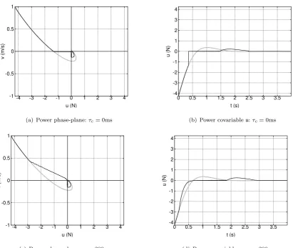
Figure 1 corresponds to pmax = 0; the input power flow must be negative, such that the

controller is semi-active, and the constraint boundaries are the axes of the power phase-plane.

Figure 1(a)&(b) correspond to a zero constraint horizonτc = 0. The unconstrained and

power-constrained trajectories are identical until the constraint boundary is reached; from this point,

-1 -0.5 0 0.5 1

-4 -3 -2 -1 0 1 2 3 4

v (m/s)

u (N)

(a) Power phase-plane:τc= 0ms

-4 -3 -2 -1 0 1 2 3 4

0 0.5 1 1.5 2 2.5 3 3.5

u (N)

t (s)

(b) Power covariableu:τc= 0ms

-1 -0.5 0 0.5 1

-4 -3 -2 -1 0 1 2 3 4

v (m/s)

u (N)

(c) Power phase-plane:τc= 200ms

-4 -3 -2 -1 0 1 2 3 4

0 0.5 1 1.5 2 2.5 3 3.5

u (N)

t (s)

(d) Power covariableu:τc= 200ms

Figure 1. Simple oscillator: transient response with initial conditionv = 1,y = 0 (39),u=−4.25 (40) andpmax = 0.

(a) With a zero constraint horizonτc= 0, the constrained, active control, trajectory (black) closely follows the unconstrained

trajectory (grey) or constraint boundarypmax= 0 as appropriate. (b) The corresponding control signaluhas a corresponding

“corner” not exhibited in the unconstrained control. (c) With a non-zero constraint horizonτc = 200ms, the constrained

trajectory (black) leaves the unconstrained trajectory before the constraint is reached thus anticipating the constraint. (d) The corresponding control signaluis smoother than that of (a)

unconstrained again. The power covariable u = u has a discontinuity when the boundary is

reached.

To investigate the effect of a non-zero constraint horizon Figure 1(c)&(d) show the effect of

a 200ms constraint horizonτc = 0.2. The unconstrained and power-constrained trajectories are

identical until the constraint boundary is approached; from this point, the power-constrained

trajectory diverges from the unconstrained trajectory and gives a smoother approach to the

constraint boundary than corresponding toτc = 0. The power covariable u=u no longer has a

discontinuity.

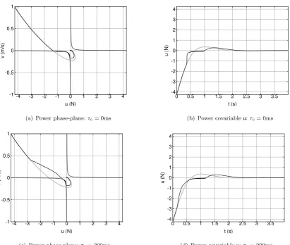
Figure 2 is similar to Figure 1 except that the power constraint is relaxed by settingpmax =

0.01. The constraint boundaries are now the rectangular hyperbolae shown in Figure 2(a)–(d)

but otherwise the behaviour is similar to that described by Figure 1. However, the smoother

-1 -0.5 0 0.5 1

-4 -3 -2 -1 0 1 2 3 4

v (m/s)

u (N)

(a) Power phase-plane:τc= 0ms

-4 -3 -2 -1 0 1 2 3 4

0 0.5 1 1.5 2 2.5 3 3.5

u (N)

t (s)

(b) Power covariableu:τc= 0ms

-1 -0.5 0 0.5 1

-4 -3 -2 -1 0 1 2 3 4

v (m/s)

u (N)

(c) Power phase-plane:τc= 200ms

-4 -3 -2 -1 0 1 2 3 4

0 0.5 1 1.5 2 2.5 3 3.5

u (N)

t (s)

(d) Power covariableu:τc= 200ms

Figure 2. Simple oscillator: transient response with initial conditionv= 1,y= 0 (39),u=−4.25 (40) andpmax= 0.01.

In contrast to Figure 1 the non-zero maximum power leads to the hyperbolic constraints leaving the axes around the origin. (a) Again, the constrained trajectory (black) closely follows the unconstrained trajectory (grey) or constraint boundary. (b) The smoother constraint leads to a smoother control signal than that of Figure 1(b). (c) and (d), as in Figure 1 , the non-zero constraint horizonτc= 200ms gives smoother control.

Figures 1(b)&(d).

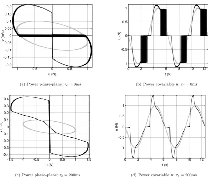
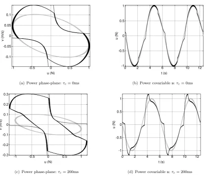
Figures 3&4 correspond to Figures 1&2 except that the initial condition is zero and the

disturbance d is a sinusoidal disturbance at the resonant frequency d = sinω0t where w0 =

1 rads−₁

. The figures display two periods after a steady-state has been reached.

Figures 3(a)&(b) show that a zero constraint horizon τc = 0 and a zero power constraint

pmax= 0 once again lead to a discontinuous control signal and, once again, this disappears when

τc = 0.2. Figures 3(a)&(c) also show the increase in the amplitude of the system velocityv=v

due to the imposition of the power constraints. Figure 4 shows the effect of relaxing the power

constraint (pmax= 0.01) in the sinusoidal disturbance case. The smoother hyperbolic constraint

boundaries give a smoother shape to the trajectories and no discontinuities are observed in the

control signals shown in Figures 4(b)&(d). Moreover, Figures 4(a)&(c) show that the relaxed

-0.2 -0.15 -0.1 -0.05 0 0.05 0.1 0.15 0.2

-1 -0.5 0 0.5 1

v (m/s)

u (N)

(a) Power phase-plane:τc= 0ms

-1 -0.5 0 0.5 1

0 2 4 6 8 10 12

u (N)

t (s)

(b) Power covariableu:τc= 0ms

-0.4 -0.3 -0.2 -0.1 0 0.1 0.2 0.3 0.4

-1.5 -1 -0.5 0 0.5 1 1.5

v (m/s)

u (N)

(c) Power phase-plane:τc= 200ms

-1 -0.5 0 0.5 1

0 2 4 6 8 10 12

u (N)

t (s)

(d) Power covariableu:τc= 200ms

Figure 3. Simple oscillator: steady-state sinusoidal response:pmax = 0. This figure corresponds to Figure 1 but with a

sinusoidal disturbance at the resonant frequencyd= sin 2πf0t. (a) With a zero constraint horizonτc= 0, the constrained

trajectory (black) lies within the negative power quadrants. (b) The corresponding control signaluexhibits a rapid switching, or chattering, phenomenon not exhibited in the unconstrained control. (c) With a non-zero constraint horizonτc= 200ms,

the constrained trajectory (black) anticipates the constraint. (d) The corresponding control signaluis smoother than that of (a) and does not exhibit chattering. In both cases, the control signal has a small high-frequency component which we attribute to deficiencies in the numerical optimisation.

3(a)&(c).

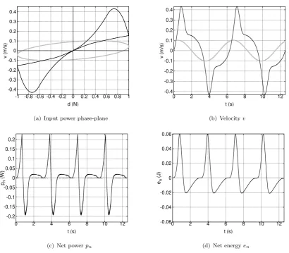
Each point on the power phase-plane trajectories of Figures 3(a), 3(c), 4(a) and 4(c)

corre-sponds to the instantaneous power p = uv associated with the control signal u and extracted

from the system. The corresponding power injected into the system by the disturbance d is

p₀ =dvand is thus, throughv, dependent on the control strategy as well asditself; this injected power can itself be represented on the power phase-plane. The net power into the system pn,

and the corresponding accumulated energyen are given by

pn(t) =p(t) +p0(t) =v(t)[u(t) +d(t)] (41)

en(t) =

Z t

0

-0.1 -0.05 0 0.05 0.1

-1 -0.5 0 0.5 1

v (m/s)

u (N)

(a) Power phase-plane:τc= 0ms

-1 -0.5 0 0.5 1

0 2 4 6 8 10 12

u (N)

t (s)

(b) Power covariableu:τc= 0ms

-0.3 -0.2 -0.1 0 0.1 0.2 0.3

-1 -0.5 0 0.5 1

v (m/s)

u (N)

(c) Power phase-plane:τc= 200ms

-1 -0.5 0 0.5 1

0 2 4 6 8 10 12

u (N)

t (s)

(d) Power covariableu:τc= 200ms

Figure 4. Simple oscillator: steady-state sinusoidal response:pmax= 0.01.This figure corresponds to Figure 2 but with a

sinusoidal disturbance at the resonant frequencyd= sin 2πf0t. In contrast to Figure 3 the non-zero maximum power leads

to the hyperbolic constraints leaving the axes around the origin. (a) The constrained trajectory (black) closely follows the unconstrained trajectory (grey) or constraint boundary. (b) The smoother constraint leads to a smoother control signal than that of Figure 3(b). (c) and (d) the trajectory no longer follows the constraints so closely.

In this particular example, the system does not, by itself, dissipate energy as there is no damping

term in Equation (34). Therefore, in the steady state, the net energy loss in the system over

one period must be zero. Figure 5 examines these ideas with reference to the particular example

of Figures 3(c) and 3(d) (pmax = 0, τc = 200ms). Figure 5(a) gives the power phase-plane

corresponding todthus the disturbance powerp₀; it corresponds to Figure 3(c) which shows the control power p; as p0 depends on velocity v (Figure 5(b)) it depends on the control strategy

as well as the disturbance d. Figure 5(c) shows the net power pn (41) as a function of time t

and Figure 5(d) shows the corresponding accumulated energyen. As predicted, the accumulated

energy is zero at the end of each period of the the disturbanced. Compared to the example in

Figures 3(a) and 3(b) (whereτc = 0), the velocities are larger and so the power injected by the

disturbance and extracted by the controller are larger. Similar results are obtained for the other

-0.4 -0.3 -0.2 -0.1 0 0.1 0.2 0.3 0.4

-1 -0.8 -0.6 -0.4 -0.2 0 0.2 0.4 0.6 0.8 1

v (m/s)

d (N)

(a) Input power phase-plane

-0.4 -0.3 -0.2 -0.1 0 0.1 0.2 0.3 0.4

0 2 4 6 8 10 12

v (m/s)

t (s)

(b) Velocityv

-0.2 -0.15 -0.1 -0.05 0 0.05 0.1 0.15 0.2

0 2 4 6 8 10 12

pn

(W)

t (s)

(c) Net powerpn

-0.06 -0.04 -0.02 0 0.02 0.04 0.06

0 2 4 6 8 10 12

en

(J)

t (s)

(d) Net energyen

Figure 5. Power and energy:pmax = 0,τc= 200ms. This Figure corresponds to Figures 3(c) and 3(d); as before, black

corresponds to constrained and grey to unconstrained control. (a) shows the power phase-plane corresponding to the dis-turbanced; this lies within the first and third quadrants indicating power inflow. (b) shows the corresponding velocity. (c) Shows the net power flowpn =v(u+d) into the system whenτc= 0 corresponding to (d) shows the corresponding

accumulated energyen=

Rt

0pn(t′)dt′. Note that the accumulated energy returns to zero at the end of each period,

4.2 Quarter car model

The quarter-car model of Figure 6 is used by Preumont (2002) as an example for illustrating

passive, active and semi-active vibration control. The same example is used by Gawthropet al.

(2012) to illustrate semi-active control based on switched intermittent control.

To make the problem more realistic, and to illustrate the case where the power covariable

u6=u, the actuator is modelled by the low-pass filter with transfer function G(s) given by

G(s) = 1

1 + 0.01s (43)

The state-space equations are of the form of Equation (1) wherez3 is the filter state and:

x=hv₂ z₂ v₁z₁ z₃ iT

m

k

c

M

K

v

v

v

f

z

z

Figure 6. Quarter car model.m= 240kg,M = 36kg,k= 16kN/m,K= 160kN/m,c= 980Nsec/m. z1 andz2 are the

spring extensions in m andv1 andv2are the mass velocities in m/s.f is an external applied force andu=−f whereuis the active control signal.

The matricesA,B,Bd andC are then given by:

A=           

−_mc −_mk _mc 0 _m1

1 0 −1 0 0

c M k M − c M − K M − 1 M

0 0 1 0 0

0 0 0 0 −100

          

, B=

           0 0 0 0 100           

, Bd=

           0 0 0 −1 0           

, C=

           1 0 0 0 0            T (45)

In this case, the power covariables are the actuator forceu=ζ and velocityv=v2−v1 hence:

Cu =

h

0 0 0 0 1 i

, Du= 0, Cv =

h

1 0−1 0 0 i

, Dv = 0 (46)

An unconstrained intermittent controller was designed as in Section 2, equation (7), with the

following parameters:

Q=hCCT i

, R= 1 (47)

Together with the system parameters of (45), these parameters give:

k=h0.43−0.26 0.0059−1.9 0.016 i

(48)

This gives closed-loop poles at: s =−2.57±j7.42, s =−13.92±j67.84 and s =−99.91. The

open-loop intermittent interval (11) was chosen as ∆i = ∆ol= 0.01s.

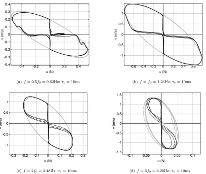
The power-constrained intermittent control was designed as in Section 3.2. Figure 7

gives the steady-state response of the system to the disturbance d = sinωt where ω =

-0.4 -0.3 -0.2 -0.1 0 0.1 0.2 0.3 0.4

-0.4 -0.2 0 0.2 0.4

v (m/s)

u (N)

(a) f= 0.5f0= 0.62Hz:τc= 10ms

-1 -0.5 0 0.5 1

-0.6 -0.4 -0.2 0 0.2 0.4 0.6

v (m/s)

u (N)

(b)f=f0= 1.24Hz:τc= 10ms

-1 -0.5 0 0.5 1

-0.3 -0.2 -0.1 0 0.1 0.2 0.3

v (m/s)

u (N)

(c)f= 2f0= 2.48Hz:τc= 10ms

-1.5 -1 -0.5 0 0.5 1 1.5

-0.1 -0.05 0 0.05 0.1

v (m/s)

u (N)

(d)f= 5f0= 6.20Hz:τc= 10ms

Figure 7. Quarter-car model: steady-state sinusoidal response. (a)–(d) give the power-phase plane sinusoidal response at 4 frequencies including the two resonant frequencies. In each case, the constrained trajectory (black) lies within the constraint boundaries (grey hyperbolae) whereas the unconstrained trajectory lies outside the constraints in three of the four cases. The use of a non-zero constraint horizon (τc= 10ms) avoids the rapid switching, or chattering, phenomenon associated with

zero horizon (τc = 0ms) but means that the trajectory does not necessarily follow the constraints closely. The maximum

powerpmaxwas set to zero.

7(a)–(d) shows the power phase-plane at each of the four frequencies for four periods when

the simulation has reached a steady-state. In each case, the power-constrained intermittent

con-troller follows the unconstrained concon-troller when away from constraints and closely follows the

constraints when the unconstrained controller violates the constraints. As discussed in Section

4.1, the use of a non-zero constraint horizon of 10ms (τc = 0.01) avoids discontinuous control.

There are, however, two discrepancies to be explained. Firstly, the constraints are violated at

certain times; this is due to the combination of the disturbance and non-zero intermittent interval

∆ol. The constraint prediction equation (22) assumes d= 0 and so the predicted constraint is

in error; this effect increases with ∆ol. The effect could be reduced by using a disturbance

model within, for example, a disturbance observer. Secondly, the four displayed periods are not

identical. This is because the disturbance period is not an integer multiple of the intermittent

-0.4 -0.3 -0.2 -0.1 0 0.1 0.2 0.3 0.4

-0.6 -0.4 -0.2 0 0.2 0.4 0.6

v (m/s)

u (N)

(a) f= 0.5f0= 0.62Hz:τc= 10ms

-1 -0.5 0 0.5 1

-0.8 -0.6 -0.4 -0.2 0 0.2 0.4 0.6 0.8

v (m/s)

u (N)

(b)f=f0= 1.24Hz:τc= 10ms

-1 -0.5 0 0.5 1

-0.4 -0.3 -0.2 -0.1 0 0.1 0.2 0.3 0.4

v (m/s)

u (N)

(c)f= 2f0= 2.48Hz:τc= 10ms

-1.5 -1 -0.5 0 0.5 1 1.5

-0.1 -0.05 0 0.05 0.1

v (m/s)

u (N)

(d)f= 5f0= 6.20Hz:τc= 10ms

Figure 8. Quarter-car model: sensitivity. This figure corresponds to Figure 7 except that the system has been multiplied by a gain of 1.2 (i.e. a 20% increase) without modifying the controller. The control system is robust to this perturbation insofar as the response is not greatly changed by this unmodelled gain.

the phase-plane statex is not periodic.

Figure 8 corresponds to Figure 7 except that the system has been multiplied by a gain of 1.2

without modifying the controller to take account of this change. The control system is robust to

this perturbation insofar as the response is not greatly changed by this unmodelled gain.

5 Conclusion

It has been shown that constraining the power flow into a dynamic system can be implemented

using quadratic constraints within a finite-horizon optimisation scheme to give power-constrained

intermittent control. Although using a zero-length constraint horizon and a strictly passive limit

on the power flow gives clipped-optimal like behaviour, a non-zero constraint horizon gives

a smoother anticipatory action. Moreover, relaxing the power limit to allow a small positive

power flow similarly gives a smoother control signal. We anticipate that the power-constrained

vibration control and low-power control using energy harvesting or regeneration.

A general purpose non-linear optimisation algorithm was used in this work and, although

suitable for demonstrating the concepts using simulations, it is neither efficient nor suitable for

real-time use. It would be of interest to take advantage of the specific quadratically-constrained

quadratic programming (QCQP) form of the optimisation and use the corresponding efficient

algorithms (Boyd and Vandenberghe 2004, Lobo et al. 1998). The high-frequency component

of the control signal visible in Figures 3 and 4 is also believed to be due to deficiencies in the

optimisation algorithm. It would therefore be of interest to investigate the exact source of this

phenomenon. The example of Section 4.2 illustrated that the method is robust to a quite large

change in system gain. Future work will provide a theoretical analysis of robustness to system

variation.

As illustrated in Section 4, there are a number of design parameters to be chosen including

the constraint horizonτc and the maximum powerpmax. In this paper, these two parameters are

chosen in anad hoc manner; future work will formulate design rules for such parameters.

Because the controller constrains the power injected into the system, the resulting constrained

controller has passivity properties even if the underlying unconstrained design does not. This is

a generalisation of the argument behind semi-active control and will be investigated to give new

generalisations of semi-active control.

Constrained control leads to considerations offeasibility. This topic has been investigated in the

context of model-based predictive control with linear constraints using quadratic programming

(Scokaertet al.1999, Mayneet al.2000) and needs to be applied to the QCQP based algorithms

discussed here.

The algorithm presented here has a fixed interval ∆i= ∆ol. However, as discussed by Gawthrop

and Wang (2009a), event-driven versions may be derived. This “control on demand” approach

may also have implications for low-energy control and will be further investigated.

The power phase-plane approach of Seth and Flowers (1990) has been shown in Section 4 to

provide a useful way of presenting the properties of the method. Future work will consider the

power phase-plane approach in more detail including the relation between the power phase-plane

of the control signal and that of the disturbance and the relative shapes of the constrained and

unconstrained cases.

Although this work was largely motivated by semi-active damping and its implementation

using modulated dampers, implementation issues are not discussed in this paper. In particular,

when the power constraint (22) is relaxed so thatpmax>0, the resultant controller can no longer

be implemented by a modulated damper. However, future work will investigate whether such a

for example, discussed by Potteret al. (2011).

This paper has been orientated towards the mechanical engineering application of semi-active

vibration control. However, it is applicable to any physical domain, or multiple physical domains,

where energy considerations are important.

Acknowledgements

Peter Gawthrop is a Visiting Research Fellow at the University of Bristol. He is also partially

supported by the linked EPSRC Grants EP/F068514/1, EP/F069022/1 and EP/F06974X/1

“Intermittent control of man and machine” and gratefully acknowledges the many discussions

about intermittent control with Henrik Gollee, Ian Loram and Martin Lakie. The authors wish

to thank Irina Lazar, University of Bristol, for her constructive comments on the draft of this

paper.

The authors gratefully acknowledge the many insightful comments of the referees which have

References

Anderson, B.D.O., and Vongpanitlerd, S., Network Analysis and Synthesis: A Modern Systems

Theory Approach, First published 1973 by Prentice-Hall, Dover (2006). ˚

Astr¨om , K.J. (2008), “Event Based Control,” in Analysis and Design of Nonlinear Control

Systemseds. A. Astolfi and L. Marconi, Heidelberg: Springer, pp. 127–147.

Bemporad, A., and Morari, M. (1999), “Robust model predictive control: A survey,” (Vol. 245,

eds. A. Garulli and A. Tesi, Springer, pp. 207–226.

Boyd, S., and Vandenberghe, L.,Convex optimization, Cambridge Univ Press (2004).

Cairano, S.D., Bemporad, A., Kolmanovsky, I.V., and Hrovat, D. (2007), “Model predictive

con-trol of magnetically actuated mass spring dampers for automotive applications,”International

Journal of Control, 80, 1701–1716.

Cannon, M., Kouvaritakis, B., and Rossiter, J. (2001), “Efficient active set optimization in triple

mode MPC,”Automatic Control, IEEE Transactions on, 46, 1307 –1312.

Cassidy, I.L., Scruggs, J.T., and Behrens, S. (2011), “Optimization of partial-state feedback for

vibratory energy harvesters subjected to broadband stochastic disturbances,”Smart Materials

and Structures, 20, 085019.

Chen, W.H., and Gawthrop, P.J. (2006), “Constrained predictive pole-placement control with

linear models,”Automatica, 42, 613–618.

Eaton, J.W.,GNU Octave Manual, Bristol: Network Theory Limited (2002).

Fialho, I.J., and Balas, G.J. (2000), “Design of nonlinear controllers for active vehicle suspensions

using parameter-varying control synthesis,”Vehicle System Dynamics, 33, 351–370.

Fletcher, R.,Practical Methods of Optimization. 2nd Edition, Chichester: Wiley (1987).

Gawthrop, P., Loram, I., Lakie, M., and Gollee, H. (2011), “Intermittent Control: A

Computa-tional Theory of Human Control,” Biological Cybernetics, 104, 31–51.

Gawthrop, P., and Wang, L. (2011), “The system-matched hold and the intermittent control

separation principle,”International Journal of Control, 84, 1965–1974.

Gawthrop, P.J. (2009), “Frequency Domain Analysis of Intermittent Control,” Proceedings of

the Institution of Mechanical Engineers Pt. I: Journal of Systems and Control Engineering,

223, 591–603.

Gawthrop, P.J., Neild, S.A., and Wagg, D.J. (2012), “Semi-active damping using a hybrid control

approach,”Journal of Intelligent Material Systems and Structures, Published online February

21, 2012.

Gawthrop, P.J., and Wang, L. (2006), “Intermittent predictive control of an inverted pendulum,”

Gawthrop, P.J., and Wang, L. (2007), “Intermittent Model Predictive Control,”Proceedings of

the Institution of Mechanical Engineers Pt. I: Journal of Systems and Control Engineering,

221, 1007–1018.

Gawthrop, P.J., and Wang, L. (2009), “Constrained intermittent model predictive control,”

International Journal of Control, 82, 1138–1147.

Gawthrop, P.J., and Wang, L. (2009a), “Event-driven Intermittent Control,”International

Jour-nal of Control, 82, 2235 – 2248.

Gawthrop, P.J., and Wang, L. (2010), “Intermittent redesign of continuous controllers,”

Inter-national Journal of Control, 83, 1581–1594.

Giorgetti, N., Bemporad, A., Tseng, H.E., and Hrovat, D. (2006), “Hybrid model predictive

control application towards optimal semi-active suspension,”International Journal of Control,

79, 521–533.

Goodwin, G., Graebe, S., and Salgado, M.,Control System Design, New Jersey: Prentice Hall

(2001).

Hong, K.S., Sohn, H.C., and Hedrick, J.K. (2002), “Modified skyhook control of semi-active

suspensions: A new model, gain scheduling, and hardware-in-the-loop tuning,” Journal of

Dynamic Systems Measurement and Control-Transactions of the ASME, 124, 158–167.

Hrovat, D. (1997), “Survey of advanced suspension developments and related optimal control

applications,” Automatica, 33, 1781–1817.

Jalili, N. (2002), “A comparative study and analysis of semi-active vibration-control systems,”

Journal of Vibration & Acoustics-Transactions of the ASME, 124, 593–605.

Jansen, L.M., and Dyke, S.J. (2000), “Semiactive control strategies for MR dampers:

Compar-ative study,”Journal of Engineering Mechanics—ASCE, 126, 795–803.

Johnson, S.G.,The NLopt nonlinear-optimization package, MIT, http://ab-initio.mit.edu/nlopt

(2012).

Karnopp, D., Crosby, M., and Harwood, R. (1974), “Vibration control using semi-active force

generators,”ASME Journal of Engineering for Industry, 96, 619–626.

Kitching, K.J., Cole, D.J., and Cebon, D. (2000), “Performance of a semi-active damper for

heavy vehicles,” Journal of Dynamic Systems Measurement & Control—Transactions of the

ASME, 122, 498–506.

Kwakernaak, H., and Sivan, R.,Linear Optimal Control Systems, New York: Wiley (1972).

Lavei, J., Rantzer, A., and Low, S. (2011), “Power flow optimization using positive quadratic

programming?,” in Proc. 18th IFAC World Congress, Milano, August.

Lobo, M.S., Vandenberghe, L., Boyd, S., and Lebret, H. (1998), “Applications of second-order

Maciejowski, J.,Predictive Control with Constraints, Prentice Hall (2002).

Matveev, A., and Yakubovich, V. (1997), “Nonconvex Problems of Global Optimization:

Linear-Quadratic Control Problems with Linear-Quadratic Constraints,”Dynamics and Control, 7, 99–134.

Mayne, D., Rawlings, J., Rao, C., and Scokaert, P. (2000), “Constrained model predictive control:

Stability and optimality,” Automatica, 36, 789–814.

Montestruque, L.A., and Antsaklis, P.J. (2003), “On the model-based control of networked

sys-tems,” Automatica, 39, 1837 – 1843.

Nakano, K., Suda, Y., and Nakadai, S. (2003), “Self-powered active vibration control using a

single electric actuator,”Journal of Sound and Vibration, 260, 213 – 235.

Potter, J.N., Neild, S.A., and Wagg, D.J. (2011), “Quasi-active suspension design using

mag-netorheological dampers,” Journal of Sound and Vibration, 330, 2201 – 2219, Dynamics of

Vibro-Impact Systems.

Powell, M.J.D. (1998), “Direct search algorithms for optimization calculations,”Acta Numerica,

7, 287–336.

Preumont, A.,Vibration control of active structures: an introduction, 2nd ed., Vol. 96 of Solid

Mechanics and its Applications, Dordrecht: Kluwer (2002).

Qin, S.J., and Badgwell, T.A. (2003), “A survey of industrial model predictive control

technol-ogy,” Control Engineering Practice, 11, 733 – 764.

Rantzer, A. (2011), “Distributed control using positive quadratic programming,” in Control

Conference (CCC), 2011 30th Chinese, Hefei, july, pp. 1 –4.

Ronco, E., Arsan, T., and Gawthrop, P.J. (1999), “Open-Loop Intermittent Feedback Control:

Practical Continuous-time GPC,”IEE Proceedings Part D: Control Theory and Applications,

146, 426–434.

Sammier, D., Sename, O., and Dugard, L. (2003), “Skyhook and H-infinity control of semi-active

suspensions: Some practical aspects,”Vehicle System Dynamics, 39, 279–308.

Scokaert, P.O.M., Mayne, D.Q., and Rawings, J.B. (1999), “Suboptimal model predictive control

(feasibility implies stability),” IEEE Trans. on Automatic Control, 44, 648–654.

Scruggs, J.T., Taflanidis, A.A., and Iwan, W.D. (2007a), “Non-linear stochastic controllers for

semiactive and regenerative systems with guaranteed quadratic performance boundsPart 1:

State feedback control,”Structural Control and Health Monitoring, 14, 1101–1120.

Scruggs, J.T., Taflanidis, A.A., and Iwan, W.D. (2007b), “Non-linear stochastic controllers for

semiactive and regenerative systems with guaranteed quadratic performance boundsPart 2:

Output feedback control,” Structural Control and Health Monitoring, 14, 1121–1137.

Seth, B., and Flowers, W.C. (1990), “Generalized Actuator Concept for the Study of the

233–238.

Shen, Y., Golnaraghi, M.F., and Heppler, G.R. (2006), “Semi-active vibration control schemes

for suspension systems using magnetorheological dampers,” Journal of Vibration & Control,

12, 3–24.

Soliman, M., Malik, O., and Westwick, D. (2011), “Ensuring Fault Ride Through for Wind

Turbines with Doubly Fed Induction Generator: a Model Predictive Control Approach,” in

18th IFAC World Congress, Milan, pp. 1710–1715.

Spencer, B.F., and Nagarajaiah, S. (2003), “State of the art of structural control,” Journal of

Structural Engineering-ASCE, 129, 845–856.

Tucker, M., and Fite, K. (2010), “Mechanical damping with electrical regeneration for a powered

transfemoral prosthesis,” in Advanced Intelligent Mechatronics (AIM), 2010 IEEE/ASME

International Conference on, Montreal, ON, july, pp. 13 –18.

Verros, G., Natsiavas, S., and Papadimitriou, C. (2005), “Design optimization of quarter-car

models with passive and semi-active suspensions under random road excitation,” Journal of

Vibration & Control, 11, 581–606.

Wang, L. (2001), “Continuous Time Model Predictive Control Using Orthonormal Functions,”

Int. J. Control, 74, 1588–1600.

Wang, L., Model Predictive Control System Design and Implementation Using MATLAB, 1st

ed., Springer (2009).

Wang, Y., and Inman, D.J. (2011), “Comparison of Control Laws for Vibration Suppression

Based on Energy Consumption,” Journal of Intelligent Material Systems and Structures, 22,

795–809.

Willems, J.C. (1972), “Dissipative Dynamical Systems, Part I: General Theory, Part II: Linear

System with Quadratic Supply Rates,”Arch. Rational Mechanics and Analysis, 45, 321–392.

Yakubovich, V.A. (1992), “Nonconvex optimization problem: The infinite-horizon

linear-quadratic control problem with linear-quadratic constraints,”Systems and Control Letters, 19, 13 –

22.

Yang, G.Q., Spencer, B.F., Jung, H.J., and Carlson, J.D. (2004), “Dynamic modeling of

large-scale magnetorheological damper systems for civil engineering applications,” Journal of