Adjusting for unrecorded consumption in survey and per capita sales data: quantification of impact on gender- and age-specific alcohol-attributable fractions for oral and pharyngeal cancers in Great Britain.

(1)

This is a repository copy of

Adjusting for unrecorded consumption in survey and per capita

sales data: quantification of impact on gender- and age-specific alcohol-attributable

fractions for oral and pharyngeal cancers in Great Britain.

.

White Rose Research Online URL for this paper:

http://eprints.whiterose.ac.uk/80828/

Article:

Meier, P.S., Meng, Y., Holmes, J. et al. (4 more authors) (2013) Adjusting for unrecorded

consumption in survey and per capita sales data: quantification of impact on gender- and

age-specific alcohol-attributable fractions for oral and pharyngeal cancers in Great Britain.

Alcohol and Alcoholism, 48 (2). 241 - 249.

https://doi.org/10.1093/alcalc/agt001

[email protected] https://eprints.whiterose.ac.uk/ Reuse

Unless indicated otherwise, fulltext items are protected by copyright with all rights reserved. The copyright exception in section 29 of the Copyright, Designs and Patents Act 1988 allows the making of a single copy solely for the purpose of non-commercial research or private study within the limits of fair dealing. The publisher or other rights-holder may allow further reproduction and re-use of this version - refer to the White Rose Research Online record for this item. Where records identify the publisher as the copyright holder, users can verify any specific terms of use on the publisher’s website.

Takedown

If you consider content in White Rose Research Online to be in breach of UK law, please notify us by

(2)

1

Adjusting for unrecorded consumption in survey and per capita sales data: Quantification of

impact on gender- and age-specific alcohol attributable fractions for oral and pharyngeal cancers

in Great Britain

Meier, Petra Sylvia1

Meng, Yang1

Holmes, John1

Baumberg, Ben2

Pursehouse, Robin.3

Hill-McManus, Daniel1

Brennan, Alan1

Author affiliations: 1 _{School of Health and Related Research (ScHARR), University of Sheffield, UK,} 2_{School of Social Policy, Sociology and Social Research (SSPSSR), University of Kent,}3 _{Department of}

Automatic Control & Systems Engineering, University of Sheffield

Corresponding author: Dr. John Holmes, 0044 114 2226384, [email protected]

(3)

2

ABSTRACT

Aims: Large discrepancies are typically found between per capita alcohol consumption estimated via

survey data compared to sales, excise or production figures. This may lead to significant inaccuracies

when calculating levels of alcohol-attributable harms. Using British data, we demonstrate an approach to

adjusting survey data to give more accurate estimates of per capita alcohol consumption.

Methods: First, sales and survey data are adjusted to account for potential biases (e.g. self-pouring,

under-sampled populations) using evidence from external data sources. Second, survey and sales data

are aligned using different implementations of Rehm et al.’s method (2010a). Third, the impact of our approaches is tested by using our revised survey dataset to calculate alcohol attributable fractions (AAF)

for oral and pharyngeal cancers.

Results: British sales data underestimates per capita consumption by 8%, primarily due to illicit alcohol.

Adjustments to survey data increase per capita consumption estimates by 35%, primarily due to

under-sampling of dependent drinkers and underestimation of home-poured spirits volumes. Before aligning

sales and survey data, the revised survey estimate remains 22% lower than the revised sales estimate.

Revised AAFs for oral and pharyngeal cancers are substantially larger with our preferred method for

aligning data sources, yielding increases in AAF from the original survey dataset of 0.47 to 0.60 (male)

and 0.28 to 0.35 (female).

Conclusions: It is possible to use external data sources to adjust survey data to reduce underestimation

of alcohol consumption and then account for residual underestimation using a statistical calibration

technique. These revisions lead to markedly higher estimated levels of alcohol-attributable harm.

Key words: per capita consumption, survey, under-coverage, alcohol attributable fraction,

methodology

Acknowledgements

This research was funded by the Medical Research Council and Economic and Social Research Council (grant G000043). The authors would also like to acknowledge the valuable contributions made by 2011

(4)

3

INTRODUCTION

The most reliable source of information on alcohol consumption is usually considered to be data on

average per capita consumption derived from official production, sales and/or customs figures (Gmel and

Rehm 2004). However, such data are population-level and can only provide aggregated per capita

consumption estimates for the total adult or drinker population. The main alternative, weighted and

grossed data from population surveys, is known to substantially underestimate population-level figures

(Knibbe and Bloomfield 2001; Nelson et al. 2010)and the reasons for this have been discussed

extensively in the survey methods literature (Duffy and Waterton 1984; Midanik 1988; Midanik 1989;

Greenfield et al. 2000; Caetano 2001; Del Boca and Darkes 2003; Gmel and Rehm 2004).

Advances in survey methods research have demonstrated means to raise the coverage of survey

estimates closer to population-level estimates through the use of diary surveys (Poikolainen and

Karkkainen 1983; Lemmens et al. 1988; Heeb and Gmel 2005), recent recall questions (Stockwell et al.

2004; Stockwell et al. 2008) and more detailed instruments or adjustment of measures (Kuhlhorn and

Leifman 1993; Casswell et al. 2002; Kerr and Greenfield 2007). However, although the impact of using

alternative measures can be dramatic (e.g. Casswell et al. 2002; Stockwell et al. 2008), other approaches

have produced only small improvements (Wyllie et al. 1994; Gmel and Rehm 2004). Consequently,

researchers still contend with residual under-coverage and must often utilise surveys with adequate

measures but potentially important biases relating to sampling methods. To date, little attention has been

given to adjusting data to account for these issues.

Despite its weaknesses, survey data allows subgroup analysis of populations and their drinking patterns

and also permits consumption distributions to be established for the population and subpopulations.

Whilst the ability to undertake subgroup analyses of consumption data has particular importance for

policy appraisals, consumption distributions are essential for calculating the proportion of an

alcohol-related harm which could be avoided if the population consumed no alcohol. This proportion is known as

the alcohol attributable fraction (AAF) and is a key component of burden of harm estimates (Rehm et al.

2009).

This paper reports on a proposed approach to adjusting survey data to account for under-coverage and

further steps to align survey and population-level data. It aims to, firstly, derive best estimates for both

aggregate per capita and survey consumption, secondly, test approaches to calibrating survey

consumption to per capita estimates and, finally, test the impact of such adjustments on UK AAF

estimates.

(5)

4

Before describing our data sources and the details of our proposed approach, a brief overview of our

method is provided. Both survey data and more accurate population-level estimates suffer from known

biases; therefore, the first step of our approach is to apply adjustments to each of these estimates by

drawing on alternative sources of evidence. This process yields a revised survey dataset and also a

revised population-level consumption estimate. We then obtain optimally-adjusted survey datasets by

aligning the revised survey to the population-level estimate using different implementations and

adaptations of a method proposed by Rehm et al (2010). Finally, we test the impact of our approach and

these various implementations by using the optimally-adjusted datasets to calculate gender- and

age-specific AAFs for oral and pharyngeal cancers.

Data

Sales data

UK clearance data is produced by Her Majesty’s Revenue and Customs (HMRC) and includes per capita consumption estimates for beer, wine, spirits and cider for adults (16+). Data collection methods are

reported elsewhere (HMRC 2010a), but the data broadly account for all alcohol released by producers or

importers for sale or consumption in the UK. This includes alcohol produced or purchased abroad for UK

sale but excludes personal imports and alcohol produced in the UK for export markets. HMRC 2006/07

data are used here.

Survey data

The General Household Survey (GHS) is an annual nationally-representative cross-sectional survey of

people living in around 9,000 private households in Great Britain (GB, i.e. the UK excluding Northern

Ireland) (ONS 2009b). Alcohol questions are asked to all adult (16+) household members using

beverage-specific quantity-frequency questions. GHS 2006 data are used here.

Table 1 shows per capita consumption estimates from the HMRC and GHS data. Coverage by GHS

relative to HMRC is 61.8% and varies markedly by beverage.

[Table 1 about here]

Adjusting population-level sales data

Previous work has noted a range of potential under- and over-estimating biases with sales data (Single

and Giesbrecht 1979; Smith et al. 1990; Greenfield and Kerr 2003) and Table 2 summarises those

relevant to the UK. Below, we outline an approach to adjusting the sales data to account for each

potential bias in turn.

(6)

5

Unrecorded alcohol

HMRC recently assessed tax loss through cross-border shopping and illicit alcohol sales for spirits and

beer (HMRC 2010b). For spirits in 2006/7 HMRC estimates cross-border trade accounted for 4% and

illicit sales for 9% of the total spirits market. For beer, 13% of the market was illicit and <1% was

cross-border trade. An alternative source, the International Passenger Survey (IPA), estimates cross-cross-border

trade in beer to account for 1.1% of duty payable (ONS 2010b). The more precise IPA estimate for

cross-border beer trade was used here. To date, HMRC has not provided estimates for wine. Alternative

data sources were found to be unsuitable; therefore, it was assumed that wine has the same level of illicit

and cross-border trade as spirits.

Although the European Comparative Alcohol Study found 0.9% of UK respondents have consumed

home-distilled spirits three or more times in the past 12 months (Leifman 2001), no UK estimates for

quantity of consumption of homemade alcohol were identified. Estimates of homemade consumption for

other countries vary markedly (Macdonald et al. 1999; Nordlund and Osterberg 2000; Stockwell et al.

2008) and, again, often only relate to prevalence, as opposed to quantity, of consumption. UK industry

and market research company sources felt that the market share was likely to be negligible so no

adjustment was made.

Ethanol content assumptions

Beer and spirits clearances do not require ethanol content assumptions as excise duty returns to HRMC

contain this information. For wine, HMRC improved their methodology for estimating wine strengths in

2010 and applied this retrospectively to sales estimates from previous years (HMRC 2008). _Therefore,

we attempted no further adjustments.

Spillage and wastage

Research by the Department of Environment, Food and Rural Affairs estimates 6% of alcoholic drinks

bought in the off-trade are wasted (DEFRA 2010). No beverage-specific rates or corresponding on-trade

data were available so we assume equal wastage for all beverages in the on- and off-trade.

Alcohol used in food

Analyses of alcohol used in food suggest alcohol content decreases by varying amounts depending on

the method of food preparation (Augustin et al. 1992), with a 50% loss on average. The National Diet and

Nutrition Survey shows that 1% of consumption occurs through food (ONS 2005), leaving 0.5% of total

consumption lost in food preparation.

(7)

6

For Scotland and England, estimates of average consumption by 11-15 year-olds were derived from

school surveys and then multiplied by mid-year population estimates (ONS 2008; ONS 2010a) to obtain

estimates of total ethanol consumption by under-16s. Separate drinking data for Wales was not available

for 2006, so English estimates were used. Overall, it was estimated that 0.7% of alcohol sold in the UK is

drunk by 11-15 year olds.

Tourism

Alcohol consumption by outbound UK tourists is missing from the HMRC sales figures, whilst

consumption by inbound tourists is included. The IPA estimates that, in 2006, foreign tourists spent

273.4m nights in the UK, whilst UK residents spent 701.3m nights abroad (ONS 2010b). It was

conservatively assumed that UK citizens abroad continue to drink the average per capita amount for

2006 (Table 1). Based on per capita consumption estimates for key source countries (BBPA 2009),

inbound tourists were assumed to drink 8.5 l/ethanol per capita per annum. Annual consumption was

converted to daily consumption and multiplied by tourist nights to estimate total tourist consumption.

Adjusting Survey Consumption

Although much of the underestimation literature focuses on evaluating survey instruments, various

additional sources of potential bias affecting survey data on alcohol consumption have been noted (Smith

et al. 1990; Caetano 2001; Gmel and Rehm 2004). Table 3 lists sources we sought to explore and we

particularly focus on adjusting or augmenting the data to ensure it is representative of all British adults.

Non-sampled populations

The GHS is a survey of private households; thus many populations, potentially containing

disproportionate numbers from heavy or light drinking demographic groups (e.g. older women) or

disproportionately heavy or light drinking elements of those groups (e.g. university students), are

excluded from the sampling frame (Wilson 1981; Duffy and Waterton 1984). We attempted to obtain best

estimates of age- and sex-specific population size and beverage-specific alcohol consumption for five

such populations (homeless, military personnel, inpatient of mental health institutions, elderly people in

care homes and prisoners). Full details of this process, which often involved merging data from multiple

sources and making adjustments and extrapolations to account for missing or incompatible information in

one of more of England, Scotland or Wales, are provided as supplementary data.

Under-sampled populations

In addition to non-sampled populations, we also investigated population suspected to be

(8)

7

Students

We focused on the 1.8m undergraduate students (HESA 2011) who are more likely to live in university

halls of residence outside the GHS sampling frame (ONS personal communication). After weighting, GHS

contains 877,000 undergraduates, just 49% of the population.

Students in the GHS consume around 20% more alcohol per year than comparable non-students of the

same age and gender and this is in line with student-specific surveys (e.g. Bewick et al. 2008). We

adjust the survey weights of present students so that they also represent missing students, thus

assuming that alcohol consumption does not differ by missingness.

Dependent drinkers

For England, the 2004 ANARP study estimated that there were 1.1m dependent drinkers (AUDIT score

>=16); 3.6% of the adult population. For Scotland, a similar study estimated 206,000 dependent drinkers,

7.2% of the adult population, with 65% being male (Drummond et al. 2005; Drummond et al. 2009).

Assuming the same prevalence in Wales as in England gives 1.37m dependent drinkers in GB.

Only one UK-based estimate of dependent drinkers’ consumption levels was identified (Gill et al. 2010).

This used an in-treatment sample and reported annual consumption levels of 109 and 89 l/ethanol per

capita for males and females respectively. AUDIT scores were not reported, thus it was not possible to

assess the sample’s position on the dependency spectrum. To establish whether the GHS accurately represents dependent drinkers, a lower threshold was set for dependent drinking at twice the UK health

service’s threshold for harmful drinking (114 g/day for men and 86 g/day for women). Even at this lower

threshold, the GHS population only contains 505,000 dependent drinkers. Dependent drinkers were

reweighted to account for underrepresentation and, to avoid double-counting, this was done after

accounting for other non-sampled or under-sampled populations.

Proxy interviews

Proxy interviews account for 7.5% of the GHS sample, and, although core demographic data is collected,

alcohol consumption is not. Proxy interviewees were particularly likely to be young and male. A two-step

multiple imputation procedure was applied to first impute whether proxy respondents were abstainers or

drinkers and, second, impute the consumption level of the drinkers (Gelman and Hill 2007) using the ice

command in Stata 11.1 (Royston 2004). In doing so, it was assumed that, after accounting for

demographic covariates, the likelihood of being a proxy respondent is not associated with alcohol

consumption. Multiple imputation was performed before testing whether students and dependent

drinkers are under-covered to avoid double counting.

(9)

8

Assumed size of self-poured drinks

Several studies have examined whether drinkers self-pour larger drinks than is assumed by survey

measures. A recent UK study around Edinburgh (Gill and Donaghy 2004) reports on asking drinkers to

pour their normal measures of spirits and wine. On average participants poured 160ml of wine

(approximately 2 units or 16g of ethanol) and 57ml of spirits (approximately 2.3 units). These findings

have been closely replicated in other Scottish studies (Gill et al. 2007). For wine, this is consistent with

GHS assumptions of 2 units for an unspecified glass of wine. However, the GHS assumption for spirits

was 1 unit per drink, thus off-trade spirit consumption amongst our sample was multiplied by 2.3 and no

adjustment was made for other beverages.

Fieldwork timing

Surveys continue throughout summer, Christmas and weeks containing public holidays; therefore, no

adjustments are required for heavy drinking periods (ONS personal communication).

Ethanol content assumptions

In 2006, conversion factors used to convert quantity measures into units of alcohol in the GHS were

updated to account for changes in beverage strengths and serving sizes, in particular for wine where

glass sizes have substantially increased (Goddard 2005). Given these recent improvements and no

further evidence of biases, no additional adjustment was made.

Revising GHS and HMRC consumption

After identifying the necessary adjustments above, the HMRC population-level estimate was revised by

calculating the net effect of the adjustments. To revise the GHS 2006 dataset there were four sequential

steps. Firstly, the consumptions for proxy interviewees were imputed. Secondly, new records were

added representing the missing populations. For each country, gender and age subgroup, eleven

additional records were created representing one abstainer and ten drinkers with their consumption

following gamma distribution (Skog 1993; Rehm et al. 2010). Population weights were set to the missing

population each added record represents. Thirdly, the weights of under-sampled populations were

adjusted uniformly in line with the above estimates. Finally, underestimation of self-poured spirits was

accounted for by multiplying all drinkers’ off-trade spirits consumption by 2.3. An upper consumption threshold of 156 l/ethanol per year was set to exclude outliers.

As a validation, the revised GHS population of England was compared to mid-year population estimates

(ONS 2010a). The overall match for the adult population improved from 89.3% to 99.9%.

(10)

9

Adjusting both population-level and individual-level consumption data does not eliminate

under-estimation by survey data (see results). Therefore, we sought to use statistical calibration techniques to

align the GHS to the HMRC estimate. An approach proposed by Rehm et al. (Method 1) shifts the survey

consumption distribution to fit a gamma function defined by the sales data and allows for differential

under-coverage rates for different observed consumption levels (Rehm et al. 2010). Further, it ensures

the adjusted population consumption follows the recommended gamma distribution (Skog 1993). Method

1 is underpinned by three assumptions. Firstly, that sales data accurately reflect per capita consumption;

secondly, population subgroups of interest do not have differential levels of under-estimation and, thirdly,

the proportion of abstainers in the survey is accurate as only known drinkers can be adjusted. Our

previous adjustments address the first assumption; however, we have no means to verify the other

assumptions.

Two limitations of Method 1 are the lack of empirical evidence to indicate under-coverage is distributed as

implied by the shifts necessary to fit adjusted consumption levels to the gamma distribution and that

shifting the consumption to a gamma distribution can artificially reduce the distribution’s long tail of heavy

drinkers. Given the latter limitation, we developed a method (Method 2) of fitting a gamma function to

the survey data and then, for each percentile of the distribution, calculating the percentage consumption

increase between this gamma distribution and the distribution given using Method 1 and then applying

these percentage shifts to the corresponding percentile of the survey data to obtain an aligned dataset.

Both Method 1 and Method 2 were employed to align the GHS data with the HMRC estimate.

Method 1 is described in more detail in Rehm et al. (2010). For our purposes, calibration was performed

separately for each country/gender/age subgroup and for each beverage type. All beverages were shifted

by the same factor which was calculated using the population mean consumption in the revised GHS and

the HMRC consumption estimate (see Table 7).

Calculating AAFs for Oral and Pharyngeal cancer

The impact of our approach to adjust and align survey and population-level data was assessed by using

various base cases and implementations of Methods 1 and 2 to calculate and compare gender- and

age-specific AAFs for oral and pharyngeal cancer.

The relative risk functions for oral and pharyngeal cancer mortality are taken from recent meta-analysis

(Tramacere et al. 2010). We are grateful to Irene Tramacere for providing by personal communication

the equation for this function (Equation 1):

ln

Where RR is the relative risk of oral and pharyngeal cancer and is daily alcohol consumption in grams.

Because individual-level survey data and continuous risk functions were used, the standard formula for

(11)

10

surveyed individuals, the relative risk estimates for consumption groups with the estimates for surveyed

individuals at their consumption level and the proportion of the population exposed in each group with a

proportion representing the individual survey weight as a percentage of the total weight in the population

(Equation 2):









1 1

1

n i i i n i i i

p RR

AAF

p RR

 











₍₂₎

Where i and n represent surveyed individuals and the total number of individuals, RRi is the relative risk

of exposure to alcohol for individual i given their consumption level, piis the proportion of the survey

weight for individual i as a percentage of the total population weight.

AAFs were calculated under eight scenarios using different versions of the GHS dataset aligned to 70%,

80% and 90% of HMRC estimates. Aligning to 70%, 80% and 90% of the HMRC estimate, rather than

100%, is done because the risk functions underpinning AAFs are derived from survey data subject to

unknown levels of underestimated consumption. Therefore, we follow recommendations to align to 90%

(Rehm et al. 2010) and use other percentages as sensitivity analyses. The first two scenarios use the

original GHS (S1) and the GHS revised but not aligned to HMRC data (S2). Scenarios 3-8 align the

revised GHS to 70%, 80% and 90% of the revised HMRC sales estimates using Method 1 (S3-S5) and

Method 2 (S6-S8).

RESULTS

Revised HMRC sales estimates

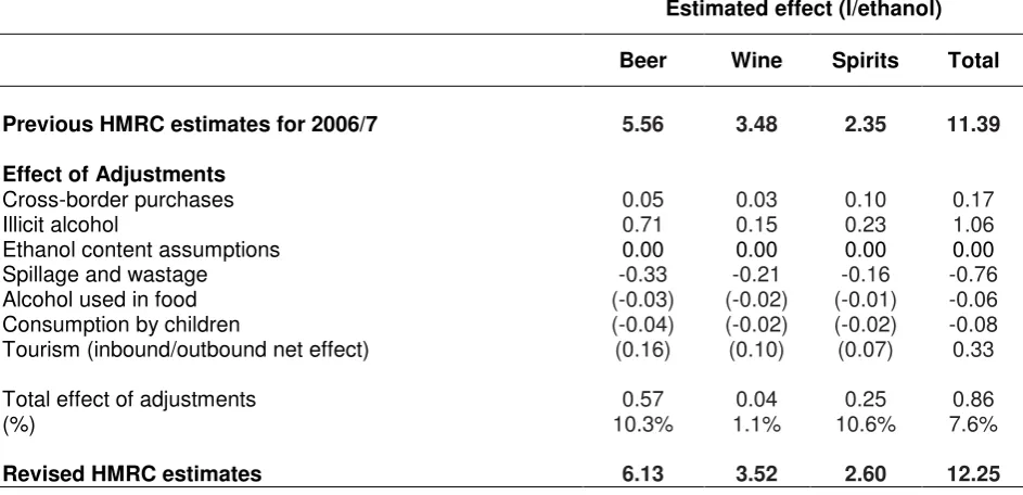
The impact of adjustments made to the aggregate-level consumption figures are shown in Table 4.

Several adjustments have only minor effects. None of cross-border purchases, alcohol used in food or

children’s consumption influenced per capita estimates by more than 2%. In contrast, tourism (+2.9%),

spillage (-6.7%) and illicit alcohol (+9.3%) have larger, but partly off-setting, impacts. The net effect of

these adjustments influences beer and spirits in particular, while the estimate for wine is largely

unchanged. The final consumption estimate of 12.3 l/ethanol per capita is 7.6% higher than the original

HMRC figure.

Revised survey consumption

The gender and age breakdown and average consumption for each subgroup of the non-sampled

population and the original GHS 2006 data, are provided in Table 5. In total, 861,000 people were

estimated to be outside the GHS sampling frame, including 230,000 homeless people (mean

(12)

11

psychiatric inpatients (4.4 l/ethanol), 400,000 care home residents (3.2 l/ethanol) and 86,000 prisoners

(1.7 l/ethanol). The weighted average annual consumption of these populations was estimated as 9.5

l/ethanol per person. Although this is 35% higher than the GHS average of 7.0 l/ethanol, the new cases

represent only 2% of the population and thus increase per capita consumption by just 0.04 l/ethanol.

The 1,513 proxy interviewees were disproportionately young and male with a predicted average

consumption of 9.0 l/ethanol, thus increasing the total GHS estimate by 0.20 l/ethanol. Reweighting for

the missing half of GB undergraduates contributed only a small increase (0.03l/ethanol); however, the

missing majority of dependent drinkers substantially increased the GHS estimate by 1.01 l/ethanol.

Adjusting for home serving sizes of spirits also had a marked effect, increasing the GHS estimate by 1.19

l/ethanol.

After carrying out all adjustments the per capita consumption estimate in the revised GHS increased by

2.47 l/ethanol or 35.1% (Table 6).

[Table 6]

Aligning GHS survey data to HMRC population-level estimates

Table 7 shows the revised survey estimates and shifting factors obtained under scenarios S1-S8. As

Methods 1 and 2 only affect the shape and not the mean of the aligned consumption distribution, the

revised estimates are identical for some scenarios. Aligning to 70%, 80% and 90% of the revised HMRC

estimate increases our revised GHS survey estimate by a further 22%, 39% and 57% respectively,

suggesting considerable residual under-estimation remained even after our initial adjustments.

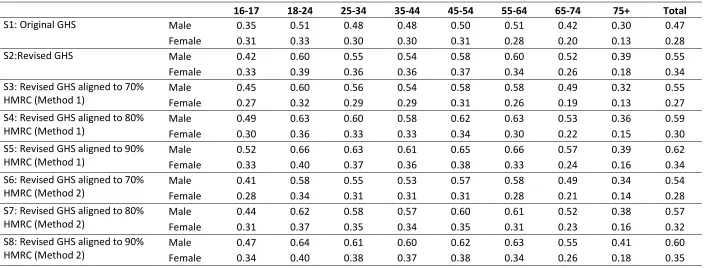
Comparison of AAFs for oral and pharyngeal cancer

Table 8 summarizes gender- and age-specific AAFs for GB oral and pharyngeal cancer mortality under 8

scenarios. The comparison shows that AAF estimates are highest in S8 when the revised survey data are

shifted to 90% of the revised HMRC sales data using Method 2. The AAFs in S8 are 0.60 for men and

0.35 for women compared with 0.47 and 0.28 respectively in S1 when the original survey data was used.

As one would expect, S1 gives the lowest AAFs suggesting underestimation of consumption in surveys

leads to underestimation of alcohol-attributable harm. In general, Method 2, which preserves the long tail

of the consumption distribution, yields higher AAFs compared with Method 1 which shifts to a continuous

gamma distribution. The decision of whether to calibrate to 70%, 80% or 90% of the HMRC data also has

a significant impact on the AAFs. The AAFs increased from 0.54 (male) and 0.28 (female) at 70% to 0.60

(13)

12

DISCUSSION

This paper has three major findings, which have relevance to the British case through the specific results

and for alcohol research more broadly through the methodological developments. Firstly, it was

estimated that per capita consumption in Britain for 2006/7 was 12.3 l/ethanol per year; 7.6% more than

the original HMRC estimate. Some potential biases had only a small impact, whilst the more important

factors somewhat offset one another. Accounting for spillage reduced the total amount drunk (-6.7%) but

this was outweighed by tourism (+2.9%) and illicit alcohol (+9.3%). The findings provide some support for

those who have queried the accuracy of per capita data although, in Britain at least, the overall impact is

modest due to counteracting biases. Many of the adjustments are, however, based on weak or

incomplete evidence and it would be informative to similarly assess the net effect of biases in other

countries with different data sources.

Secondly, a new survey-based estimate of average consumption was produced that corrected for a

number of potential biases and raised survey consumption by 35%, but still left residual underestimation.

Some biases had smaller effects than expected; notably, accounting for the consumption of around

860,000 people not living in private households increased per capita consumption by just 0.6%, mainly

because of counteracting adjustment and most of the added populations being fairly small. However,

these missing populations represent many of society’s heaviest and lightest drinkers and accounting for them may have substantial effects on AAFs and thus estimated levels of alcohol-related harm. Adjusting

for other sampling biases had a larger effect, particularly under-sampling of dependent drinkers which

increased average consumption by 14.4% and we recommend further research to improve prevalence

and consumption estimates for this group. Accounting for under-estimation of self-poured off-trade spirits

(16.9% increase) was also important and highlights the importance of surveys using robust instruments.

Casswell et al. (2002) have demonstrated that underestimation is not a given with survey instruments,

although their method is unfeasibly time-consuming for some surveys. Greenfield et al. (2010) have

achieved high coverage rates with a less intensive calibrated graduated frequency approach and further

methodological developments which lead to robust and efficient survey instruments would be welcome.

Finally, adjusting survey consumption has a significant impact on estimates of AAFs for oral and

pharyngeal cancer. As expected, using adjusted survey data and further aligning it to population-level

sales data gives higher AAF estimates than using unadjusted survey data. This strongly suggests

estimated levels of alcohol-related harm based on population surveys may contain sizeable

underestimates of true levels of harm. Aligning to sales data by calibrating the survey consumption

distribution to a gamma distribution of the sales data is seen to artificially reduce the long tail of heavy

consumption and thus results in lower AAFs than our adapted approach which preserves the empirical

consumption distribution. Thus, we believe our adapted method to be the preferable approach. Those

using harm estimates based on survey data should be aware of the potential biases which are

(14)

13

as the WHO Global Burden of Disease studies, do already adjust survey data with reference to sales or

excise records (Rehm et al. 2007).

Limitations

For several adjustments, there was substantial uncertainty due to a lack of robust evidence; for example,

drinking by tourists and wastage estimates for the on-trade sector. For survey estimates, this uncertainty

affected the most important biases such as off-trade spirits servings and the prevalence and consumption

levels of dependent drinkers. Further research should focus on obtaining robust estimates in these

areas.

Due to limited data availability and the scale and complexity of this study, we have not performed a

comprehensive sensitivity analysis to address the uncertainty of our revised consumption estimates.

Ideally we would obtain a range of revised estimates using different data sources and assumptions and

obtain confidence intervals where possible. However, the importance of this is reduced as, unless the

uncertainty and confidence intervals are large, their impact on our findings should be limited given we are

aligning survey consumption to 70% to 90% of the revised HMRC and this uncertainty will dominate other

uncertainties. That said, uncertainty regarding individual-level GHS adjustments will impact on subgroup

level AAF estimates where adjustments relate to specific population subgroups such as dependent

drinkers or students.

Further limitations include assuming constant under-coverage when adjusting survey consumption in

different subpopulations or for different beverages for many of the considered biases. It should also be

noted that, although we address under-sampling of dependent drinkers, we assume harmful drinkers are

adequately represented.

CONCLUSION

Of the biases investigated, we find those impacting most on consumption estimates are under-sampling

of dependent drinkers and under-estimation of home-poured spirits volumes. We demonstrate a method

for adjusting both sales and survey data to obtain revised consumption estimates and present a means

for aligning survey data to population-level data to account for residual under-estimation. We also

highlight the importance of retaining the long tail of the consumption distribution. Overall, we

demonstrate that practicable and evidence-based methods for accounting for underestimation of alcohol

consumption lead to substantially increased estimates of the proportion of given harms attributed to

(15)

(16)

15 References

Augustin J, Augustin E, Cutrufelli RL, Hagen SR and Teitzel C. (1992) Alcohol retention in food

preparation.

J Am Diet Assoc

,

92:

_486-8

BBPA. (2009)

Statiscal Handbook: A compilation of drinks industry statistics

London: Brewing

Publications Limited.

Bewick BM, Mulhern B, Barkham M, Trusler K, Hill AJ and Stiles WB. (2008) Changes in undergraduate

student alcohol consumption as they progress through university.

BMC Public Health

,

8:

₁₆₃

Caetano R. (2001) Non-response in alcohol and drug surveys: a research topic in need of further

attention.

Addiction

,

96:

_1541-5

Casswell S, Huckle T and Pledger M. (2002) Survey Data Need Not Underestimate Alcohol Consumption.

Alcoholism: Alcohol Clin Exp Res

,

26:

_1561-7

Communities and Local Government. (2010) Statutory Homelessness: 3rd Quarter (July to September)

2010, England. http://www.communities.gov.uk/publications/corporate/statistics/homelessnessq32010

DEFRA. (2010)

Household Food and Drink Waste linked to Food and Drink Purchases

.

Department for

Envrionment, Food and Rural Affairs.

Del Boca FK and Darkes J. (2003) The validity of self-reports of alcohol consumption: state of the science

and challenges for research.

Addiction

,

98:

_Suppl-12

Drummond C, Deluca P, Oyefeso A, Rome A, Scarfton S and Rice P. (2009)

Scottish Alcohol Needs

Assessment

.

London: Institute of Psychiatry, King's College London:

Drummond C, Oyefeso A, Phillips T, Cheeta S, Deluca P, Perryman K, Winfield H, Jenner J, Cobain K,

Galea S, Saunders V, Fuller T, Pappalardo D, Baker O and Christoupoulos A. (2005)

Alcohol Needs

Assessment Research Project (ANARP): The 2004 National Alcohol Needs Assessment for

England

.

London: Department of Health:

Duffy JC and Waterton JJ. (1984) Under-reporting of alcohol consumption in sample surveys: the effect

of computer interviewing in fieldwork.

Brit J Addict

,

79:

_303-8

Gelman A and Hill J. (2007)

Data Analysis Using Regression and Multilevel/Hierarchical Models

Cambridge University Press.

Gill J and Donaghy M. (2004) Variation in the alcohol content of a 'drink' of wine and spirit poured by a

sample of the Scottish population.

Health Educ Res

,

19:

_485-91

Gill J, Tsang C, Black H and Chick J. (2010) Can Part of the Health Damage Linked to Alcohol Misuse in

Scotland be Attributable to the Type of Drink and its Low Price (by Permitting a Rapid Rate of

Consumption)? A Point of View.

Alcohol Alcoholism

,

45:

_398-400

Gill JS, Donaghy M, Guise J and Warner P. (2007) Descriptors and accounts of alcohol consumption:

methodological issues piloted with female undergraduate drinkers in Scotland.

Health Educ Res

,

22:

27-36

(17)

16 Goddard E. (2005)

Estimating alcohol consumption from survey data: updated method of converting

volumes to units

.

London, Office for National Statistics:

Greenfield T and Kerr WC. (2003) Tracking Alcohol Consumption Over Time.

http://pubs.niaaa.nih.gov/publications/arh27-1/30-38.htm

Greenfield, T., Nayak, M. B., Bond, J., Patel, V., Trocki, K., and Pillai, A. Validating alcohol use measures

among male drinkers in Goa: Implications for research on alcohol, sexual risk, and HIV in India. AIDS

Behaviour 14, S84-S93. 2010.

Greenfield TK, Midanik LT and Rogers JD. (2000) Effects of telephone versus face-to-face interview

modes on reports of alcohol consumption.

Addiction

,

95:

_277-84

Heeb JL and Gmel G. (2005) Measuring alcohol consumption: a comparison of graduated frequency,

quantity frequency, and weekly recall diary methods in a general population survey.

Addict Behav

,

30:

403-13

HESA. (2011) Students in Higher Education Institutions 2006/7.

http://www.hesa.ac.uk/index.php?option=com_pubs&task=show_pub_detail&pubid=1&Itemid=286

HMRC. (2008)

Review of wine strengths used in estimating pure alcohol clearances

.

London: HM

Revenue & Customers:

HMRC. (2010a)

Alcohol Factsheet 2010

.

London: HM Revenue & Customs:

HMRC. (2010b) Measuring tax gaps 2010.

http://www.hmrc.gov.uk/stats/measuring-tax-gaps-2010.htm.pdf

Jones L, Bellis MA, Dedman D, Sumnall H and Tocque K. (2008)

Alcohol-attributable fractions for

England: alcohol-attributable mortality and hospital admissions

.

Liverpool: Liverpool John Moores

University, Centre for Public Health.

Kerr WC and Greenfield TK. (2007) Distribution of alcohol consumption and expenditures and the

impact of improved measurement on coverage of alcohol sales in the 2000 National Alcohol Survey.

Alcohol Clin Exp Res

,

31:

_1714-22

Knibbe RA and Bloomfield K. (2001) Alcohol Consumption Estimates in Surveys in Europe: Comparability

and Sensitivity for Gender Differences.

Substance Abuse

,

22:

_23-38

Kuhlhorn E and Leifman H. (1993) Alcohol surveys with high and low coverage rate: a comparative

analysis of survey strategies in the alcohol field.

J Stud Alcohol

,

54:

_542-54

Leifman H. (2001) Estimations of unrecorded alcohol consumption levels and trends in 14 European

countries.

Nord Stud Alcohol Drugs (Eng Suppl),

18:

_54-70

Lemmens P, Knibbe RA and Tan F. (1988) Weekly Recall and Diary Estimates of Alcohol Consumption in

a General Population Survey.

J Stud Alcohol

,

49:

_131-5

Macdonald, S., Wells, S., and Giesbrecht, N. (1999) Unrecorded alcohol consumption in Ontario, Canada:

estimation procedures and research implications.

Drug Alcohol Rev

,

18:

_21-29

Midanik LT. (1988) Validity of self-reported alcohol use: a literature review and assessment.

Brit J

Addict

,

83:

_1019-30

(18)

17 Nelson DE, Naimi TS, Brewer RD and Roeber J. (2010) US state alcohol sales compared to survey data,

1993-2006.

Addiction

,

105:

_1589-96

Nordlund S and Osterberg E. (2000) Unrecorded alcohol consumption: its economics and its effects on

alcohol control in the Nordic countries.

Addiction

,

95:

_S51-64

ONS. (2005) National Diet and Nutrition Survey : Adults Aged 19 to 64 Years, 2000-2001.

http://www.esds.ac.uk/findingData/snDescription.asp?sn=5140

ONS. (2008)

Smoking, drinking and drug use among young people in England

.

NHS Information Centre

for Health and Social Care, Leeds:

ONS. (2009a)

Annual Abstract of Statistics

.

Basingstoke: Palgrave Macmillan.

ONS. (2009b)

General Household Survey, 2006. SN: 5804. Colchester: UK Data Archive.

ONS. (2010a) Mid Year Population Estimates 2006.

http://www.statistics.gov.uk/statbase/Product.asp?vlnk=15106

ONS. (2010b) Travel Trends 2009. http://www.ons.gov.uk/ons/rel/ott/travel-trends/2009/index.html

Poikolainen K and Karkkainen P. (1983) Diary gives more accurate information about alcohol

consumption than questionnaire.

Drug Alcohol Depen

,

11:

_209-16

Rehm J, Klotsche J and Patra J. (2007) Comparative quantification of alcohol exposure as risk factor for

global burden of disaese.

Int J Meth Psych Res

,

16:

_66-76

Rehm J, Kehoe T, Gmel G, Stinson F, Grant B and Gmel G. (2010) Statistical modeling of volume of

alcohol exposure for epidemiological studies of population health: the US example.

Pop Health Metrics

,

8:

_1-12

Rehm J, Mathers C, Popova S, Thavorncharoensap M, Teerawattananon Y and Patra J. (2009) Alcohol

and Global Health 1 Global burden of disease and injury and economic cost attributable to alcohol use

and alcohol-use disorders.

Lancet

,

373:

_2223-33

Royston P. (2004) Multiple imputation of missing values.

Stata Journal

,

4:

_227-41

Single E and Giesbrecht N. (1979) The 16 per cent Solution and other Mysteries concerning the Accuracy

of Alcohol Consumption Estimates based on Sales Data .

J Addict Alcohol Drugs

,

74:

_165-73

Skog OJ. (1993) The tail of the alcohol consumption distribution.

Addiction

,

88:

_601-10

Smith PF, Remington PL, Williamson DF and Anda RF. (1990) A comparison of alcohol sales data with

survey data on self-reported alcohol use in 21 states.

Am J Public Health

,

80:

_309-12

Stockwell T, Donath S, Cooper-Stanbury M, Chikritzhs T, Catalano P and Mateo C. (2004)

Under-reporting of alcohol consumption in household surveys: a comparison of quantity-frequency,

graduated-frequency and recent recall.

Addiction

,

99:

_1024-33

(19)

18 Tramacere I, Negri E, Bagnardi V, Garavello W, Rota M, Scotti L, Islami F, Corrao G, Boffetta P and

Vecchia C. (2010) A meta-analysis of alcohol drinking and oral and pharyngeal cancers. Part 1: Overall

results and dose-risk relation.

Oral Oncol.

,

46:

_497-503

Wilson P. (1981) Improving the reliability of drinking surveys.

Statistician

,

30:

_159-67

(20)

19

Supplementary data to: Meier et al. ‘Adjusting for unrecorded consumption in survey and per capita sales data: Quantification of impact on gender- and age-specific alcohol attributable

fractions for oral and pharyngeal cancers in Great Britain’

Description of methods for obtaining estimates of the size and alcohol consumption levels of

non-sampled populations (i.e. populations who do not live in private households).

Homeless people

Official figures on homeless households in GB were obtained but only the Scottish data details household

composition (Scottish Executive 2006; Communities and Local Government 2010). This was applied to all

of GB to give a total of 149,548 officially homeless GB adults. However, official figures exclude those who

do not come into contact with authorities and this ‘hidden’ homeless population was estimated to be

83,200 individuals; giving a total of 232,748 homeless adults (Crisis 2008). Additional data sourceswere

used to estimate age and sex distributions (Warnes and Crane 2001; Scottish Executive 2006).

Estimates for gender- and age-specific alcohol consumption were based on the homelessness

supplement of the 1994 Adult Psychiatric Morbidity Survey (APMS) (OPCS 1994). To account for

consumption changes over time, each percentile of the consumption distribution was adjusted to 2006

levels based on the relative increase in each GHS percentile over the same period; thus assuming that

homeless drinking has increased at the same rate as in the general population.

Military personnel not living in private households

No figures were available detailing the housing arrangements of military personnel. However,160,500

military personnel were resident in GB during 2006 (ONS 2009a) and 42,000 of these were living in

family accommodation within the GHS sampling frame (National Audit Office 2009). It was estimated that

90 per cent of the remaining personnel would be living in single living quarters (BBC 2007)and thus

outside the GHS sampling frame. Age and sex distributions were derived from a representative survey of

military personnel conducted between 2004 and 2006 (Hotopf et al. 2006). The survey suggested military

personnel consumed similar levels of alcohol to the general population (Hooper et al. 2008). Therefore,

the gender/age specific consumption distributions from the 2006 GHS were applied.

Inpatients of mental health institutions

A 2005 census of English and Welsh mental health institutions identified 33,828 inpatients and described

sex and age data from which population distributions were derived (Healthcare Commission 2005). No

comparable population estimate for Scotland could be obtained so this was extrapolated from the

proportion of the English and Welsh population who were inpatients and the same age-sex distribution

(21)

20

As with homelessness, the 1994 APMS surveyed a representative sample of psychiatric inpatients

(OPCS 1996). The same method to derive consumption distributions was used as with the homeless.

Elderly people living in care homes

After removing Northern Irish cases, an Office of Fair Trading study estimates the GB care home

population to be 397,687 (Office of Fair Trading 2005). There is conflicting international literature as to

whether older people drink more or less after moving to a nursing home (Joseph 1995; Glass et al. 1995;

Johnson 2000) and no UK-specific evidence was identified. Therefore, the appropriate age and sex

consumption distributions from the 2006 GHS were applied.

Prisoners

Official British and Scottish prisons statistics show there were approximately 86,000 prisoners in GB at

any time in 2006, including 4,600 women (HM Prison Service 2011). Only the Scottish government

publishes an age distribution (Scottish Government 2007), so this was applied to all GB prisoners.

No alcohol consumption estimate for prisoners could be identified but HM Prison Service reports alcohol

problems are largely confined to open prisons (HM Prison Service 2004) and abstinence or

near-abstinence is common during incarceration (Parkes et al. 2011). In the absence of data, total near-abstinence

was assumed in closed prisons, and drinking at twice the government’s recommended limits was

(22)

21 References

BBC. (2007) Forces housing 'must be improved'. http://news.bbc.co.uk/1/hi/uk/6230173.stm

Crisis. (2008) Hidden Homelessness. http://www.crisis.org.uk/policywatch/pages/hidden_homeless.html

Glass TA, Prigerson H, Kasl SV and Mendes de Leon CF. (1995) The effects of negative life events on

alcohol consumption among older men and women.

J Gerentol B-Psychol

,

50:

_S205-S216

Healthcare Commission. (2005)

Count me in: Results of a census of inpatients in mental health hospitals

and facilities in England and Wales

.

London: Healthcare Commission:

HM Prison Service. (2004)

Addressing Alcohol Misuse: A prison service alcohol strategy for

prisoners

.

London: HMPS.

HM Prison Service. (2011) Population Figures.

http://www.hmprisonservice.gov.uk/resourcecentre/publicationsdocuments/index.asp?cat=85

Hooper R, Rona RJ, Jones M, Fear NT, Hull L and Wessely S. (2008) Cigarette and alcohol use in the UK

armed forces and their association with combat exposure: A prospective study.

Addict Behav

,

33:

_1067-71

Hotopf M, Hull L, Fear NT, Browne T, Horn O, Iversen A, Jones M, Murphy D, Bland D, Earnshaw M,

Greenberg N, Hughes JH, Tate AR, Dandeker C, Rona R and Wessely S. (2006) The health of UK military

personnel who deployed to the 2003 Iraq war: a cohort study.

Lancet

,

367:

_1731-41

Johnson I. (2000) Alcohol problems in old age: a review of recent epidemiological research.

Int J Geriatr

Psych

,

15:

_575-81

Joseph CL. (1995) Alcohol and drug misuse in the nursing home.

Int J Addict

,

30:

_1953-84

National Audit Office. (2009)

Ministry of Defence: Service Families Accommodation

.

London: The

Stationary Office:

Office of Fair Trading. (2005) Care homes for older people in the UK: A market study.

http://www.oft.gov.uk/OFTwork/markets-work/completed/care-homes1

OPCS. (1994)

OPCS Survey of Psychiatric Morbidity among Homeless People, 1994

.

Colchester: UK Data

Archive.

OPCS. (1996)

OPCS Surveys of Psychiatric Morbidity : Institutions Sample, 1994

.

Colchester: UK Data

Archive.

Parkes T, MacAskill S, Brooks O, Jepson R, Atherton I, Doi L, McGhee S, and Eadie D. (2011) Prison health

needs assessment for alcohol problems.

http://www.ohrn.nhs.uk/resource/policy/PrisonHealthNeedsAssessmentAlcohol.pdf

Scottish Executive. (2006) Statistical Bulletin: Housing Series.

http://www.scotland.gov.uk/Resource/Doc/149558/0039817.pdf

Scottish Government. (2007) Prison Statistics Scotland 2006/7.

http://www.scotland.gov.uk/Publications/2007/08/31102446/0

(23)

[image:23.595.65.515.140.228.2]

22 Tables

Table 2: Potential biases on UK population-level consumption estimates from HMRC sales data

Underestimating Influences Unclear direction Overestimating Influences

Unrecorded alcohol including illicit and homebrewed alcohol and cross-border purchases

Incorrect ethanol content assumptions

Spillage and wastage before and after sale

Alcohol consumed by UK tourists

abroad Alcohol used in food

Consumption by children aged under 16

[image:23.595.67.545.336.492.2]

Alcohol consumed in the UK by tourists

Table 3: Potential biases on UK consumption estimates from the GHS survey data

Unsampled populations Under-sampled populations Other biases

Homeless people

Military personnel not living in private accommodation

Inpatients of psychiatric institutions

Elderly living in care homes

Prisoners

Students

Dependent drinkers

Other possible survey non-respondents

Assumed size of self-poured drinks

Ethanol content assumptions

Fieldwork timing in relation to high consumption periods

Table 1: Beverage-specific consumption and coverage estimates by data source

HMRC 2006 per capita

GHS 2006 per

capita Coverage (%)

All alcohol 11.39 7.04 61.8

Beer & Cider 5.56 3.05 54.9

Wine 3.48 2.80 80.5

Spirits 2.35 1.18 50.2

[image:23.595.64.528.581.720.2]

(24)

[image:24.595.71.543.95.323.2]

23

Table 4: Quantification of underestimating and overestimating effects on UK per capita data

Estimated effect (l/ethanol)

Beer Wine Spirits Total

Previous HMRC estimates for 2006/7 5.56 3.48 2.35 11.39

Effect of Adjustments

Cross-border purchases 0.05 0.03 0.10 0.17

Illicit alcohol 0.71 0.15 0.23 1.06

Ethanol content assumptions 0.00 0.00 0.00 0.00

Spillage and wastage -0.33 -0.21 -0.16 -0.76

Alcohol used in food (-0.03) (-0.02) (-0.01) -0.06

Consumption by children (-0.04) (-0.02) (-0.02) -0.08

Tourism (inbound/outbound net effect) (0.16) (0.10) (0.07) 0.33

Total effect of adjustments 0.57 0.04 0.25 0.86

(%) 10.3% 1.1% 10.6% 7.6%

Revised HMRC estimates 6.13 3.52 2.60 12.25

Note: Data represent effects in l/ethanol per person per annum. Figures in brackets were not available in beverage-specific form, and have been assigned to beverage types based on the HMRC sales split.

1 _{The total alcohol net effect is made up of alcohol sold in UK but consumed by visiting tourists (-0.12 l/ethanol) and}

(25)

[image:25.595.71.519.96.683.2]

24

Table 5: Age and sex distribution, and estimated annual per capita consumption (l/ethanol) for missing populations

Male Female Total

N Mean

l/ethanol N

Mean

l/ethanol N

Mean l/ethanol Homeless

Under 18 12,146 12.4 8,261 4.6 20,407 9.2

18-24 27,402 23.0 12,240 5.1 39,642 17.5

25-34 45,823 26.7 14,068 6.2 59,890 21.8

35-44 43,355 23.0 11,923 12.9 55,278 20.8

45-54 23,350 36.7 9,059 46.3 32,410 39.4

55-64 15,809 47.7 3,519 3.2 19,328 39.6

65-74 3,029 36.9 401 2.2 3,430 32.9

75+ 1,670 23.3 333 1.6 2,003 19.8

Total 172,584 27.6 59,804 12.9 232,388 23.8

Military personnel not living in private households

18-24 15,773 7.6 1,753 4.7 17,525 7.3

25-34 38,849 11.0 4,317 5.8 43,166 10.5

35-44 30,963 10.2 3,440 5.3 34,403 9.7

45-54 11,782 10.2 1,309 5.2 13,090 9.7

Total 97,366 10.1 10,819 5.4 108,185 9.6

Inpatients of mental health institutions

18-24 1,645 12.1 1,346 5.8 2,991 9.3

25-34 3,654 3.3 2,990 3.3 6,644 3.3

35-44 3,363 6.3 2,751 1.7 6,114 4.2

45-54 2,751 5.7 2,251 1.4 5,002 3.8

55-64 2,649 13.0 2,168 0.4 4,817 7.3

65-74 3,261 6.4 2,668 0.3 5,929 3.7

75+ 3,057 3.2 2,501 0.1 5,558 1.8

Total 20,380 6.6 16,674 1.6 37,054 4.4

Elderly living in care homes

55-64 5,170 11.0 5,170 4.6 10,340 7.8

65-74 15,907 8.3 27,838 3.2 43,746 5.0

75+ 78,344 5.3 265,257 2.1 343,602 2.8

Total 99,422 6.1 298,265 2.2 397,687 3.2

Prisoners

16-17 2,565 1.75 107 1.16 2,672 1.73

18-24 21,450 1.75 1,336 1.16 22,787 1.72

25-34 27,547 1.75 1,730 1.16 29,277 1.72

35-44 19,363 1.75 1,038 1.16 20,401 1.72

45-54 7,230 1.75 310 1.16 7,540 1.73

55-64 2,374 1.75 72 1.16 2,446 1.73

65-74 823 1.75 0 1.16 823 1.75

75+ 0 0 0

Total 81,352 1.75 4,593 1.16 85,945 1.72

Total added records 861,259 9.47

Original GHS

16-17 393,757 6.85 345,969 4.69 739,725 5.84

18-24 1,860,788 10.97 2,190,406 5.83 4,051,195 8.19

25-34 3,137,187 10.19 3,517,133 5.30 6,654,319 7.61

35-44 3,919,879 10.20 4,357,863 5.18 8,277,742 7.56

45-54 3,255,828 10.67 3,790,034 5.47 7,045,861 7.87

55-64 3,194,160 10.94 3,305,257 4.63 6,499,417 7.73

65-74 2,230,197 8.23 2,482,076 3.18 4,712,273 5.57

75+ 1,606,019 5.30 2,428,465 2.07 4,034,484 3.36

(26)

[image:26.595.69.406.77.359.2]

25

Table 6. Survey adjustments: Effects on per capita consumption

Estimated effect size l/ethanol per capita

Previous GHS per capita estimate 7.04

Missing populations

Homeless +0.080

Military +0.006

Mental health institutions -0.003

Care homes -0.034

Prisons -0.010

Total +0.04

Under-coverage

Students +0.03

Dependent drinkers +1.01

Proxy interviewees +0.20

Total +1.24

Self-pouring (adjustment for off-trade spirits) +1.19

Fieldwork timing 0

Ethanol content assumptions 0

Total effect +2.47

New GHS annual per capita estimate 9.51

Table 7. Mean annual per capita consumption (l/ethanol) for the 8 scenarios and shifting factors

Annual per capita consumption Shift factor1

S1: Basecase GHS 2006 S2: Revised GHS 2006 Revised HMRC 2006 S3,S6: HMRC 2006 revised (70%) S4,S7: HMRC 2006 revised (80%) S5,S8: HMRC 2006 revised (90%)

S3,S6 S4,S7 S5,S8

Beer/cider 3.05 3.88 6.13 4.29 4.90 5.52 1.11 1.26 1.42

Wine 2.81 3.04 3.52 2.46 2.82 3.17 0.81 0.93 1.04

Spirits 1.18 2.60 2.60 1.82 2.08 2.34 0.70 0.80 0.90

Total 7.04 9.49 12.25 8.58 9.80 11.03 0.90 1.03 1.16

[image:26.595.66.532.451.602.2]

(27)

[image:27.842.59.767.94.362.2]

26

Table 8: Comparison of gender/age specific AAFs of oral and pharyngeal cancers for the UK population in 8 difference scenarios

16-17

18-24

25-34

35-44

45-54

55-64

65-74

75+

Total

S1: Original GHS

Male

0.35

0.51

0.48

0.50

0.51

0.42

0.30

0.47 Female

0.31

0.33

0.30

0.31

0.28

0.20

0.13

0.28 S2:Revised GHS

Male

0.42

0.60

0.55

0.54

0.58

0.60

0.52

0.39

0.55 Female

0.33

0.39

0.36

0.37

0.34

0.26

0.18

0.34 S3: Revised GHS aligned to 70%

HMRC (Method 1)

Male

0.45

0.60

0.56

0.54

0.58

0.49

0.32

0.55 Female

0.27

0.32

0.29

0.31

0.26

0.19

0.13

0.27 S4: Revised GHS aligned to 80%

HMRC (Method 1)

Male

0.49

0.63

0.60

0.58

0.62

0.63

0.53

0.36

0.59 Female

0.30

0.36

0.33

0.34

0.30

0.22

0.15

0.30 S5: Revised GHS aligned to 90%

HMRC (Method 1)

Male

0.52

0.66

0.63

0.61

0.65

0.66

0.57

0.39

0.62 Female

0.33

0.40

0.37

0.36

0.38

0.33

0.24

0.16

0.34 S6: Revised GHS aligned to 70%

HMRC (Method 2)

Male

0.41

0.58

0.55

0.53

0.57

0.58

0.49

0.34

0.54 Female

0.28

0.34

0.31

0.28

0.21

0.14

0.28 S7: Revised GHS aligned to 80%

HMRC (Method 2)

Male

0.44

0.62

0.58

0.57

0.60

0.61

0.52

0.38

0.57 Female

0.31

0.37

0.35

0.34

0.35

0.31

0.23

0.16

0.32 S8: Revised GHS aligned to 90%

HMRC (Method 2)

Male

0.47

0.64

0.61

0.60

0.62

0.63

0.55

0.41

0.60 Female

0.34

0.40

0.38

0.37

0.38

0.34

0.26

0.18

0.35

(28)

27