Modelling converted seismic waveforms in isotropic and anisotropic 1-D gradients: discontinuous versus continuous gradient representations

White Rose Research Online

[email protected]

Universities of Leeds, Sheffield and York

http://eprints.whiterose.ac.uk/

This is an author produced version of a paper published in

Studia Geophysica

et Geodaetica

White Rose Research Online URL for this paper:

http://eprints.whiterose.ac.uk/id/eprint/77381

Paper:

Angus, DA and Thomson, CJ (2012)

Modelling converted seismic waveforms in

isotropic and anisotropic 1-D gradients: discontinuous versus continuous gradient

representations.

Studia Geophysica et Geodaetica, 56 (2). 383 - 409. ISSN

0039-3169

Modelling converted seismic waveforms in isotropic and

anisotropic 1–D gradients: discontinuous versus continuous

gradient representations

D.A. Angus

& C.J. Thomson

1 _{School of Earth & Environment, University of Leeds, Leeds, [email protected]} 2 _{Schlumberger Cambridge Research, Cambridge, UK}

Accepted: Studia Geophysica & Geodetica: 2012

Abstract

Over the past decade, there have been numerous receiver function studies directed at imaging the lithosphere–asthenosphere boundary (LAB). Although it is generally ac-cepted that receiver function phases observed in these studies are derived from physical mode conversions at depth within the lithosphere–asthenosphere transition, it is still debatable as to whether these phases are directly indicative of the LAB. This is be-cause interpretation of receiver function LAB signals relies on understanding the elastic characteristics of the Earth’s outer thermal boundary layer. The main issues for re-ceiver function imaging are the sharpness of the elastic material property transition and, more importantly, what specifically are the material gradients. To test the various transition models, a forward modelling approach is required that allows accurate wave-form synthetics for a range of discontinuous and continuous gradients in anisotropic, elastic media. We present a derivation of the reflection and transmission response for continuous one–dimensional (1–D) gradients in generally anisotropic elastic media. We evaluate the influence of 1–D isotropic and anisotropic elastic gradients on the seismic waveform by comparing numerical results of models for discontinuous and continuous transitions. The results indicate that discontinuous representations using layers each with uniform parameters and with thicknesses on the order of approximately 1/3 to 1/8 of the dominant seismic wavelength can be used to accurately model P–to–S and S–to–P mode conversions due to continuous transitions of both isotropic and anisotropic elastic properties. From a practical point of view, when comparing synthetic modelling with observation, this constraint can be relaxed further. The presence of signal noise and/or the result of receiver function stacking techniques will likely obscure these sub-tle waveform effects. Hence this study suggest that accurate synthetic waveforms for LAB transitions can be modelled with discontinuous gradient representations using a reasonable number of discrete transition layers with layer thicknesses no greater than 1/2 to 1/3 the dominant seismic wavelength.

Key words: elastic waves, isotropic and anisotropic gradients, lithosphere– asthenosphere boundary, reflection and transmission response, Ricatti equations.

1 INTRODUCTION

The Earth is elastically anisotropic and heterogeneous over a wide range of scales and this complexity is manifested in the numerous seismic phases and their waveforms from earth-quakes. As such, analysis of teleseismic waves has become a fundamental component of global Earth studies, provid-ing constraints on the Earth’s geometry as well as thermal and chemical evolution. Due to economic and practical lim-itations on the location and size of seismic arrays as well as the uneven distribution of earthquake sources,

complex-ity of the model, for example, a reduction from elastic to acoustic media (e.g., Brenders & Pratt, 2007).

Although the Earth is heterogeneous in all three– dimensions, in a broad sense and on a global scale this het-erogeneity is predominantly depth dependent as a result of the pressure and temperature distribution within the Earth. Teleseismic mode conversions from P– and S–wave phases are ideal for studying depth dependent structure in the crust and upper mantle (e.g., Vinnik, 1977). By removing source and receiver side waveform effects via deconvolution, the re-ceiver function method (e.g., Langston, 1977) enhances any sub–vertically propagating mode conversions (i.e., P–to–S and S–to–P) and hence enables relatively high resolution vertical and potentially lateral imaging of crustal (e.g., Tom-linson et al., 2003; Angus et al., 2009) and upper–mantle discontinuities (e.g., Helffrich et al., 2003; Thompson et al., 2011). Since receiver function analysis focusses primarily on vertical structure, a reduction of the model space from three dimensions (3–D) to one–dimension (1–D) allows for a more tractable solution of the wave physics of interest (i.e., mode conversions). Reflectivity modelling [either consider-ing a spectrum of slownesses (e.g., Fuchs & Mueller, 1971) or the plane–wave response (e.g., Frederiksen & Bostock, 2000)], is often the forward modelling tool of choice in the interpretation of receiver functions and this is because it is computationally efficient and yields accurate full waveform solutions. However, more advanced methods, such as one– way wave equation techniques, are now being applied that allow for lateral variations in the topology of sub–horizontal crustal and upper–mantle discontinuities within the model (e.g., Audet et al., 2007).

Over the past decade, there has been significant in-terest in imaging the lithosphere–asthenosphere boundary (LAB) (see Fischer et al., 2010, and references therein). However, the exact definition of the lithosphere and the asthenosphere varies within the geoscience community and hence a ubiquitous definition of the LAB remains controver-sial (see Artemieva, 2009). In a general sense, the LAB rep-resents the boundary or transition within the upper mantle between the convective asthenosphere and the conductive lithosphere. Regardless of the semantics involved in defin-ing the LAB, the geophysical characteristics of this transi-tion have important implicatransi-tions on our understanding of upper–mantle convection, the outer thermal boundary layer and the evolution of plate tectonics.

Receiver function analyses using teleseismic P–to–S and S–to–P mode conversions have been used to delineate sharp sub–horizontal seismic discontinuities generally inferred to be the LAB (e.g., Farra & Vinnik, 2000; Li et al., 2004; Ku-mar et al., 2005; Rychert et al., 2005; Angus et al., 2006). In some instances, however, receiver function interpretations of the LAB have been at odds with other geophysical data, such as mantle xenolith thermal studies (Tommasi, personal communication, 2007). This suggests a better understand-ing of the mechanisms leadunderstand-ing to mode conversions at these depths and more concrete evidence to indicate whether the converted phases are truly related to the LAB, or not, is needed. Thermal models suggest a very weak and diffuse LAB leading to predicted low amplitude and broad con-verted seismic waves, and hence are inconsistent with re-ceiver function studies. However, current hypotheses sug-gest that seismic waves within this thermal transition are

sensitive to much sharper contrasts in elastic properties, such as changes in mantle hydration, chemical fertility, melt content and/or vertical gradients in elastic anisotropy (e.g., Artemieva, 2009; Fischer et al., 2010; Holtzman & Kendall, 2010). Thus, elastic gradients associated with the thermal LAB can be expected to range from smooth to relatively sharp.

2 STATEMENT OF PROBLEM

The receiver function method provides an estimate of the Earth structure in terms of a sequence of time offset mode conversions from sub-horizontal discontinuities and hence the assumption of predominantly 1–D vertical structure for individual receiver functions is generally sufficient. To cor-rectly model the seismic response due to 1–D structure one needs to consider the interaction of the incident elastic wave with a discontinuity in material properties. The energy of the primary wave can be converted into up to six secondary waves. Although Snell’s law can be used to determine the directional properties of all the secondary waves, it cannot provide information on waveform amplitudes and pulse dis-tortion. Thus a more complete evaluation of the reflection and transmission (R/T) properties is needed. Over the past several decades significant contributions have been made in the evaluation of R/T coefficients for isotropic (e.g., Gilbert & Backus, 1983; Molotkov et al., 1976; Novotn´y et al., 1980; Kennett, 1983) and anisotropic (e.g., Garmany, 1983; Fryer & Frazer, 1984; Guest et al., 1993) layered media (see Ken-nett, 2001a). In most of these approaches, the solution to the R/T response involves using a local plane–wave and plane– boundary approximation (see Hudson, 1980; Kennett, 1983). The plane–wave R/T coefficients depend only on the slow-nesses, polarizations, and material properties at the point of incidence.

gradi-ents have been shown to yield substantially complex wave-form coupling (e.g., Shearer & Chapman, 1988; Chapman & Shearer, 1989; Coates & Chapman, 1990, to name just a few studies), but how this might impact on mode conver-sions and receiver functions has yet to be examined.

In this paper, we present a derivation of the R/T re-sponse for 1–D, continuously–varying, generally anisotropic elastic media and evaluate the influence of 1–D isotropic and anisotropic elastic gradients on the seismic waveform. Specif-ically, we compare numerical results for 1–D discontinuous and continuous transitions for both isotropic and anisotropic media. The concepts presented here were initially based on Kennett (1983) for the isotropic elastic case and contribu-tions from Thomson (1996b) for both the anisotropic discon-tinuous elastic case as well as the isotropic and anisotropic continuous elastic case. The reader is referred to Kennett (2001a) for a more current overview of R/T theory and Ken-nett (2001b) for application of modelling to teleseismic data.

3 REFLECTION AND TRANSMISSION COEFFICIENTS

The theory presented here is expressed in Cartesian coordi-nates (x1, x2, x3) = (x, y, z) withz positive downwards and

summation convention implied. For an elastic medium, the linear stress–strain relation is

σij=cijkl ∂uk ∂xl

, (3.1)

wherecijklis the fourth–order tensor of elastic parameters, σij is the stress tensor, ǫkl =∂uk/∂xl is the strain tensor, uk is thek–th component of displacement, andxlis the l–

th Cartesian coordinate. For an impulsive point force with magnitudemi, located spatially and temporally at x† and t†_{, the equation of motion is}

∂σij ∂xj

=ρ∂

2_u

i

∂t2 +miδ(x−x

†

)δ(t†), (3.2) where ρis density. For 1–D media, the material properties vary only with depthz and so the source is defined atx†= (0,0, x†₃).

The 3–D Fourier transform of the displacement wave-fielduis expressed with respect to time and lateral coordi-nates

u(p1, p2, ω) =

Z Z Z ∞

−∞

u(x1, x2, t)

e[−iω(p1x1+p2x2−t)]_dx

1dx2dt , (3.3)

where p1, p2 are the lateral slowness and u(x1, x2, t) =

u(x3)e[−iω(p1x1+p2x2−t)] is the plane–wave solution for

fre-quency ω. From here on, the lateral coordinates and slow-nesses are denoted by Greek subscripts (e.g., xα and pα).

After Fourier transformation and using a modified form in-troduced by Woodhouse (1973), the equation of motion 3.2 is written in matrix form (Guest et al., 1993)

dy

dx3

= iωAy+sδ(x3−x†3)e

−iωpαxα _{, (3.4)}

where the 6–vector y= ui ti (3.5)

consists of components of displacementui and normal

trac-tionti

ui= (u1, u2, u3)T and ti=

1

iω(σ13, σ23, σ33)

T _{. (3.6)}

The system matrixAis partitioned into four 3×3 matrices as follows:

A=

TT C−₃₃1 S T

, (3.7)

where

T=−pγCγ3C−331 (3.8)

and

S=ρI−pγpα Cαγ−Cα3C−331C3γ

. (3.9) The reduced elasticity matrixCij is defined (Cik)jl=cijkl

(e.g.,C33=ci3k3). The 6×6 system matrixAis of

particu-lar importance because its eigenvectors define the displace-ments and interface tractions associated with all possible wavetypes. The corresponding six eigenvalues of A repre-sent the six possible normal slownesses (p3) to the interface

for given lateral slownesses (pα).

The expected solution in a homogeneous layer takes the form

y(z) =Neiωqzc, (3.10) whereNis a 6×6 matrix whose columns are the eigenvectors ofA,q is a diagonal matrix consisting of the correspond-ing eigenvalues andc is a column vector representing the wavevector constants for the layer defining the amplitudes of the upgoing and downgoing waves (assumed order as that of the columns ofN).

3.1 1–D discontinuous gradients

For elastic wave propagation, we require continuity of dis-placement and normal stresses across a material interface. For a single (horizontal) interface, the boundary conditions state that the wavevector z+

1 just above the interface and

z−

1 just below the interface are related by

N(z+)c+=N(z−)c−, (3.11)

neglecting the exponential term. Equation 3.11 can be ap-plied to the set of all possible incident wavesqP,qS1andqS2

(qreferring to quasi and indicating that the P–wave particle motion is not normal to the wavefront and that the S–wave motion is not parallel to the wavefront) at the interface and expressed in matrix form as

N(z+)

0 I TU RD

=N(z−)

RU TD

I 0

, (3.12)

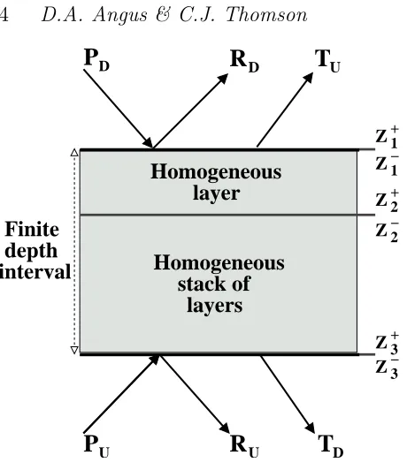
whereDrefers to downward incident waves andUto upward incident waves (see Figure 1). For example, TU is a 3×

3 matrix of transmission coefficients for all three possible transmitted waves from the three possible upgoing incident waves.

Rearranging equation 3.12, a 6×6 layer interface scat-tering matrixQis written

N−1(z−)N(z+) = Q(z−, z+) (3.13)

=

TD−RUTU−1RD RUT−U1 −T−_U1RD T−_U1

U

R

T

T

U

R

Z

Z

Z

Z

Z

Z

depth

P

interval

Finite

P

layers

Homogeneous

layer

Homogeneous

stack of

Figure 1. Cartoon of reflection and transmission matrix coeffi-cients for a finite depth interval of a homogeneous stack of hor-izontal layers.RD andTD represent the reflected and

transmit-ted plane wave from the locally plane wavePDinitially traveling

downward. RU and TU represent the reflected and transmitted

plane wave from the locally plane wavePU initially traveling

up-ward (Fryer & Frazer, 1984).

The wave propagator matrix Q is an expression of all the wavevectors in the upper and lower medium. The matrixQ can be inverted to express the 3×3 R/T matrices in terms of the 3×3 partitions of the scattering matrix denotedQ11,

Q12,Q21, andQ22, as

TU RU

RD TD

=

Q−1

22 Q12Q−221

−Q−₂₂1Q21 Q11−Q12Q−221Q21

.

(3.14)

For a stack of homogeneous layers (see Figure 1), equa-tion 3.11 can be generalized for a finite depth interval (z3, z2)

as

N(z3)c3=P(z3, z2)N(z2)c2 , (3.15)

where Pis the displacement–stress propagator within the finite depth interval. The wavevectorsc2 andc3are related

by the layer–interface scattering matrix

Q(z3, z2) = N−1(z3)P(z3, z2)N(z2) (3.16)

=

TD−RUTU−1RD RUT−U1 −T−_U1RD T−_U1

,

where the R/T matrices are those for the entire region be-tweenz2 andz3, whether it be one homogeneous layer or a

finite stack of layers. Since the propagator P is in itself a product of individual propagators for each layer, it follows that the wave propagator satisfies the chain rule

Q(z3, z1) =Q(z3, z2)Q(z2, z1). (3.17)

For a homogeneous layer of thickness h=z3−z2 the

wave propagatorQ(z3, z2) can be expressed as

E(z3, z2) =

ED 0

0 EU

(3.18)

where ED= diag

h

eiωqD1h,eiωqD2h,eiωqD3h

i

and EU= diag

h

eiωqU1h,eiωqU2h,eiωqU3h

i

.

This represents a phase lag with no amplitude modification. Using the chain rule 3.17, the R/T matrix coefficients for the depth interval below the interfacez1 to the base of

interfacez3(i.e., the region betweenz−₁ andz₃−in Figure 1)

can be expressed

_¯

TD−R¯UT¯−U1R¯D R¯UT¯−U1 −T¯−_U1R¯D T¯−_U1

= (3.19)

TD−RUTU−1RD RUT−U1 −T−U1RD T−U1

ED 0

0 EU

.

where the matrices with single overbars represent the R/T properties for the region (z−₁,z−₃). The R/T matrices without overbars represent those for region (z+

2,z

−

3) and the far right

matrices propagate the waves across the homogeneous region (z−

1,z +

2). With further simplification, the addition rules for

adding a new layer to the stack (not including the top of the interface) can be expressed as

¯

TU = E−U1TU

¯

RD = E−U1RDED

¯

RU = RU

¯

TD = TDED. (3.20)

To include the top of interfacez1 (i.e.,z−1 toz+1),

ap-plication of the chain rule gives

_˜

TD−R˜UT˜−U1R˜D R˜UT˜−U1 −T˜−_U1R˜D T˜−_U1

=

_¯

TD−R¯UT¯−U1R¯D R¯UT¯−U1 −T¯−_U1R¯D T¯−_U1

TD−RUTU−1RD RUT−U1 −T−_U1RD T−_U1

, (3.21)

where the matrices to the left of the equality (i.e., with tildes) represent the R/T matrix coefficients for the whole region (z+

1,z

−

3) and those to the right for the single interface

(z+₁,z−₁) and stack region (z₁−,z₃−). Thus, the addition rules for including the new interface are

˜

TU = TU(I−R¯DRU)−1T¯U, (3.22)

˜

TD = T¯D[I+RU(I−R¯DRU)−1R¯D]TD

= T¯D(I−RUR¯D)−1TD, (3.23)

˜

RU = R¯U+ ¯TDRU(I−R¯DRU)−1T¯U

= R¯U+ ¯TD(I−RUR¯D)−1RUT¯U, (3.24)

˜

RD = RD+TU(I−R¯DRU)−1R¯DTD

= RD+TUR¯D(I−RUR¯D)−1TD . (3.25)

invariant bedding approach in the derivation of the reflec-tion and transmission coefficients.

3.2 1–D continuous gradients

The R/T solution for continuous or higher order transitions can be approximated by dividing the transition zone into many thin homogeneous layers when the material gradients are high (Haskell, 1953; Gilbert & Backus, 1983). Another approach is to apply a phase shift neglecting amplitude ef-fects when the material gradients are small (Helffrich et al., 2008); there is minimal amplitude error when the material gradients are weak (Angus, 2004). Although this might be an efficient approach for isotropic gradients, the question re-mains as to whether it is suitable for anisotropic transitions that might arise, for instance, due to melt or strain induced anisotropy related to the Earth’s depth dependent geotherm. In this section, we introduce a formulation for the R/T re-sponse for a continuous 1–D transition. This approach is similar to the approach described by Bostock (1999), yet differs with respect to how the differential (or local) R/T matrix coefficients are evaluated. The approach of Bostock (1999) evaluates the differential R/T matrix coefficients via finite material property perturbations within a homogeneous reference medium. Here we describe and apply the approach of Thomson (1996a,b), where the differential R/T matrix coefficients are evaluated via products of the spatially lo-calized eigenvector matrices of displacement and stress, and their derivatives with respect to depth.

Development of the R/T coefficients for continuously– variable media begins with equation 3.15 for a finite layer fromz1 toz2. Differentiating with respect toz2 we have

∂ ∂z2

N(z2)

RU TD

I 0

=

∂ ∂z2

P(z2, z1)N(z1)

0 I TU RD

. (3.26)

Noting thatN(z1) is independent ofz2, utilizing the

equa-tion of moequa-tiondP/dz= iωAPand given the following initial values asz2→z1

P(z2, z1),TU,TD→I and RU,RD→0, (3.27)

equation 3.26 can be written

∂ztD ∂zrU −∂zrD −∂ztU

= iωq−N−1∂zN. (3.28)

The quantities rD,U and tD,U represent the local vertical

derivatives of the ‘thin’ layer R/T coefficients. In effect, equation 3.28 is an expression for the local vertical deriva-tives of the global R/T coefficients. The quantities q and N−1 are known but an expression for ∂zN is still needed.

Two options are available to evaluate∂zN: seek an analytic

expression or approximate the expression numerically.

3.2.1 Analytic form

An analytic expression can be found by first taking the fol-lowing derivative (equation 6.2 in Appendix A) with respect toz

∂z(AN) =∂z(Nq) (3.29)

yielding

qB−Bq=∂zq−N−1∂zAN, (3.30)

where

B=N−1∂zN . (3.31)

Equation 3.31 is referred to as the coupling matrix (Chap-man, 2004). Expression 3.30 has the useful property in that the diagonal components are zero when N is normalized to the vertical energy flux. This can be seen by taking the derivative of equation 6.12 with respect toz,

∂z(NTJN) = ∂z(NT)JN+NTJ(∂zN)

= (∂zNT)(N−1)T+N−1∂zN

= (N−1∂zN)T+N−1∂zN

= BT+B=0. (3.32) The result of which indicates thatBis antisymmetric and thus the diagonal elements ofN−1∂zNmust be zero. That

being the case, only the off–diagonal components need be determined and can be found from equation 3.30 as follows,

Bij=

(

0 i=j

(∂zq−N−1_∂zAN)

ij (qi−qj) i6=j

, (3.33)

where∂zAand∂zqhave yet to be evaluated.

The derivative of the system matrixAwith respect to z is

∂zA=∂z

TT C−₃₃1 S T

(3.34)

and can be expressed in terms of its partitions. The deriva-tive∂zC−₃₃1is found by making use of the relationC33C−331=

Isuch that

∂z(C33C−331) = (∂zC33)C33−1+C33(∂zC−₃₃1) =0 (3.35)

which yields

∂zC−331=−C

−1

33(∂zC33)C−331. (3.36)

The remaining partition derivatives (after some simplifica-tion) are

∂zT = ∂z(−pγCγ3C−331) (3.37)

= −pγ(∂zCγ3)C−331−Cγ3C−331(∂zC33)C−331

∂zTT = (∂zT)T (3.38) ∂zS = ∂zρI−pγpα Cαγ−Cα3C−331C3γ

= ∂zρI−pγpα[(∂zCαγ)−

(∂zCα3)C33−1C3γCα3C−331(∂zC33)C−331C3γ −Cα3C−331(∂zC3γ). (3.39)

There are several approaches which may be used to eval-uate the derivative of the eigenvalue matrixq with respect to z. One approach would be to differentiate the solution to the eigenvalue problem

∂z[det|A−qI|] = 0, (3.40)

since ∂zA is already known. Unfortunately this would be

rather tedious since it requires evaluating the derivative of the cofactor matrices ( ˇCerven´y, 2001; Chapman, 2004). For 1–D media the lateral slownesses (pα) remain constant with

slownesses (pα) and elastic matrix. Thus for all six

possi-ble waves the ray equations ( ˇCerven´y, 2001) can be used to evaluate∂zqfrom

∂pz ∂z =−

_∂pz

∂τ / ∂z ∂τ

, (3.41)

where∂pz/∂τ and∂z/∂τ are evaluated using the ray

equa-tions.

It is now possible to solve the coupling matrix B us-ing relation (3.33) which is clearly only valid if qi 6=qj. It

is obvious that Bij is singular along the diagonal, where qi=qjand the denominator is zero. Since the coupling

ma-trix describes how rapidly the eigenvector of the ithwave is changing with respect to that of the jthwave, the diagonal elements are not significant and can be set to zero.

Coupling occurs at interfaces and in regions of gradi-ents, and is strongest within gradients when the wave slow-nesses are approximately equal. For anisotropic media, sin-gularities will exist when the slowness sheets touch and special consideration must be taken (e.g., see Crampin & Yedlin, 1981; Shearer & Chapman, 1989; Angus et al., 2004, for intersection, kiss and conical point singularities). For the 1–D laterally isotropic case we can make use of the fact that theSH–wave is invariant and so derivatives of both the

dis-placement and stress eigenvector are zero. In other words, there is no coupling between theSH–wave and theP– and SV–waves in isotropic media. This implies that two

eigenvec-tors (columns) associated with theSH–waves be zero and,

by making use of symmetry properties, determines the cou-pling matrix.

3.2.2 Numerical approximation

Evaluation of the analytic expression can be problematic when the model consists of a transition from isotropy to anisotropy, where the denominator in equation 3.33 becomes numerically singular as the medium approaches isotropy. An alternative to the analytic expression is to evaluate the derivative numerically using a first–order accurate finite– difference stencil, e.g.,

∂zN≈ N_z+

i

−N_z−

i

∆z +O(∆z) . (3.42)

This approach is robust in terms of transitions between isotropy and anisotropy and is sufficiently accurate when ∆z

is not too large. However, implementation of this approach can be tricky when using the Runge–Kutta numerical ap-proach, where variable step size is implemented (see next section for discussion of the Runge–Kutta method).

3.2.3 The Ricatti equations

Using either the analytic form (3.31) or numerical approxi-mation (3.42) of∂zN, the derivatives of equation 3.28 yield

the approximate local vertical–gradient R/T coefficients for a thin layer to first–order with respect to thickness. These derivatives may be used with the addition rules 3.22–3.25 to obtain the global vertical–gradient R/T coefficients for a continuously–varying medium

dTU = dtuTU+RDdrUTU dTD = TDdtD+TDdrURD

dRU = TDdrUTU

dRD = drD+dtURD+RDdtD+RDdrURD (3.43)

(Thomson, 1996b). These are the Ricatti equations and are a set of non–linear first–order ordinary differential equations (similar forms have been presented by Ursin, 1983; Tromp & Snieder, 1989; Bostock, 1999).

4 NUMERICAL IMPLEMENTATION

The numerical solution of the first–order non–linear Ricatti equations (3.43) can be solved by a variety of ordinary– differential equation solvers. Problems involving ordinary differential equations, such as the Ricatti equations, can be reduced to the study of a set of first–order differential equa-tions of the form

y′= dy

dz =f(z,y) (4.1)

with initial condition

y(z0) =Γ. (4.2)

The problem is then reduced to the study of a set of N

coupled first–order differential equations. For the particular case of the Ricatti equations 3.43, the problem is reduced to a set of four coupled first–order equations of the form

dy1

dz = a1(z)y1+y4a3(z)y1 dy2

dz = y2a2(z) +y2a3(z)y4 dy3

dz = y2a3(z)y1 dy4

dz = a4(z) +a1(z)y4+y4a2(z) +y4a3(z)y4 (4.3)

where

(y1,y2,y3,y4) = (TU,TD,RU,RD) (4.4)

and

(a1,a2,a3,a4) = (dTU, dTD, dRU, dRD) . (4.5)

Given the initial conditions

y1(zo) =y2(zo) =I and y3(zo) =y4(zo) =0 (4.6)

equations 4.3 can be solved numerically.

There are a variety of numerical approaches based on Euler’s method to solve this system of first–order ordinary differential. In all approaches, the ordinary differential equa-tiony′ _{over an intervalz∈[a, b] is replaced by an algebraic}

equation of the form

k

X

j=0

αjyn+j=hφf(yn+k, yn+k−1, . . . , yn, zn;h) (4.7)

at discrete points zn defined by zn = a+nh, where n =

0,1,2, . . . , N= (b−a)/hand the step lengthhmay or may not vary (Lambert, 1991). The parameterφf is dependent

on yn+k, yn+k−1, . . . , yn, znthrough the derivative

terms of theyn+j andfn+j, j= 0,1, . . . , kparameters.

Bo-stock (1999) uses the Adams–Moulton implicit predictor– corrector multistep method to solve the Ricatti equations. In the formulation of Bostock (1999) the material proper-ties are found through model perturbations and not though any direct explicit relationship to the independent variable

z. Since the matrix coefficients are evaluated in a process independent of depth, the choice of the implicit predictor– corrector method is suitable. Furthermore, the predictor– corrector method has been observed to be relatively efficient for complicated functional forms of equations 3.43 (Bostock, personal communication, 1999).

In this paper, the formulation of the differential R/T matrix coefficients involves the products of depth localized eigenvector matrices and their derivatives. Since the deriva-tion of the differential R/T matrix coefficients are explic-itly related to the independent variablez, an ideal approach would involve implementation of a variable step length. Al-though predictor–corrector methods do allow for variable step length, they tend to be difficult to implement and less efficient than Runge–Kutta (RK) methods. RK methods re-tain the one–step format, but achieve higher order accuracy by sacrificing the linearity with respect toyn+j and fn+j.

Although there is no difficulty in varying step length, error estimation can be more complicated to evaluate compared to linear multistep methods. However, for the derivation of the R/T coefficients in this paper, the RK method is more suitable since it can efficiently drive the step length and hence the depth at which the coefficients and their deriva-tives are evaluated. Changing step length can be easily ac-commodated since the dependent variables are explicitly described in terms of depth. This can be particularly im-portant in regions with sharp gradients. [Other approaches that allow variable step size, such as the Bulirsch–Stoer al-gorithm (Press et al., 2007), may also be appropriate.] The specific RK method used in this study is Verner’s eight– stage formula pair of order 5 and 6 (Verner, 1990, 1991). This method is a modification of Fehlberg’s eight–stage for-mula pairs of order 5 and 6. The design has been modified such that the sixth–order approximation can be propagated using only eight function evaluations in each successful step (sometimes referred to as local extrapolation). Verner’s 5–6 pair is found to be a suitable and convenient choice of RK method for solving the non–linear Ricatti equations.

5 RESULTS

We examine three 1–D Earth models based on the integral error function

erf(η) = 2

π

Z η

0

exp [−(η′)2]dη′ (5.1)

(e.g., see equation 4–111, Turcotte & Schubert, 1982) com-monly used as a solution in numerous physical problems. These models represent simple conceptual models of the asthenosphere–lithosphere transition (see Figure 3). The depth extent of the entire model as well as the thickness of the lithosphere are kept constant at 200 km and 50 km, re-spectively, and only the transition thickness below the litho-sphere is varied. Model 1 is an isotropic transition consist-ing of a velocity increase between the asthenosphere and

Figure 3. Sketch of the three simple 1–D models of an asthenosphere–lithosphere transition. The models are described from the bottom up to be consistent with the direction of prop-agation of the incident and converted waves. The variable pa-rameter in model 1 is the isotropic velocity, in model 2 is the strength of anisotropy, and in model 3 is the orientation of the anisotropic symmetry axis. For simplicity, we consider constant density throughout the asthenosphere and lithosphere.

lithosphere, where the P–wave and S–wave velocities in-crease by 1% and 5%, respectively (based on Table 2 in Artemieva, 2009). Model 2 is a transition from isotropy to anisotropy, with isotropy in the asthenosphere developing into anisotropic olivine in the lithosphere. The olivine is scaled to a maximum P– and S–wave anisotropy of approxi-mately 7.5% and 5.5%, respectively, and the isotropic elastic tensor is obtained using a Voigt–Reuss–Hill average (the or-thorhombic olivine elasticity tensor is taken from Babuska & Cara, 1991, page 49). The transition from isotropy to anisotropy is accomplished by using the error function to de-fine the anisotropic scaling. For this transition, the change in vertical P–wave velocity is minimal (∆VP ≤0.2%), whereas

the S–wave velocity for vertical propagation and horizon-tal polarization increases by up to 3%. Model 3 is entirely anisotropic (7.5% and 5.5% P– and S–wave anisotropy) in both the asthenosphere and lithosphere and is loosely based on the studies of Ben Isma¨ıl & Mainprice (1998) and Black-man & Kendall (2002). The gradient is defined by a smooth rotation of the olivine elastic tensor. In the lithosphere, the fast P–wave velocity is aligned along the x–axis, the slow P–wave velocity along the y–axis and the moderate P–wave velocity along the z–axis. In the asthenosphere, the fast and moderate P–wave velocities are rotated (i.e., fast P–wave along the z–axis and the moderate P–wave along the x– axis). See Table 2 for elastic tensor coefficients for models 2 and 3.

re-Model C11 C22 C33 C12 C13 C23 C44 C55 C66

2 Litho 77.616 77.616 70.560 24.314 25.944 25.944 24.010 24.010 26.651 Asthe 70.560 70.560 70.560 22.540 22.540 22.540 24.010 24.010 24.010

3 Litho 77.616 77.616 70.560 24.314 25.944 25.944 24.010 24.010 26.651 Asthe 70.560 77.616 77.616 25.944 25.944 24.3140 26.651 24.010 24.010

Figure 2.Elastic tensor components (in GPa) for the anisotropic models 2 and 3. The elastic tensors are density normalized, where densityρ= 3311 kg/m3_.

Figure 4.Results for model 1 (isotropic transition) for incident P–wave: (a) 10 km transition and (b) 50 km transition. For this and remaining figures, the left column displays the receiver func-tion signals and the right column displays the vertical (U(Z)) and horizontal (U(X)) displacement waveforms. The grey wave-forms are from the discontinuous models, where n refers to the number of discrete layers, and the waveforms in black are from the continuous model (or Ricatti solution). Note that the primary waveforms are clipped to enhance the converted phase waveforms. As well, the amplitude of the receiver functions in Figures 3, 4 and 5 have been scaled by a factor of 2 to improve visualization of the converted waveforms.

gions containing S–wave slowness surface singularities to ex-ist.

Typical epicentral distances used in receiver function analysis range between 35◦_{and 95}◦_{for P receiver functions}

(e.g., Wilson et al., 2005) and between 60◦ _{and 75}◦ _{for S}

receiver functions (e.g., Wilson et al., 2006; Angus et al., 2006). Based on these epicentral distances, we use an inci-dence angle of 20◦_{from vertical as representative of vertical}

incidence for both teleseismic P– and S–waves. We model

Figure 5.Results for model 1 (isotropic transition) for incident S–wave: (a) 10 km transition and (b) 50 km transition.

the seismic source as a plane–wave with a Ricker wavelet having dominant (or peak) frequency of 1 Hz and 0.5 Hz for incident P– and S–waves, respectively. Based on the ve-locities used in the models (8.4 km/s for P-wave and 4.9 km/s for S-wave), the wavelengths of the P– and S–waves are approximately 8.4 km and 9.8 km, respectively. For dom-inant wavelengths on the order of 10 km for both wave types, two transition thicknesses are considered; a 50 km transition (e.g., representative of a diffuse thermal anomaly) and a 10 km transition (e.g., representative of a zone of partial melt or hydration). For all models, we present the deconvolved con-verted waveforms using the iterative time–domain technique of Ligorria & Ammon (1999) [for P–to–S conversion, we de-convolve the z–component (vertical) from the x–component, and for S–to–P conversion, we deconvolve the x–component from the z–component and reverse the time axis such that the converted P–wave trails the incident S–wave].

Figure 6. Results for model 2 (isotropic to anisotropic) tran-sition for incident S–wave: (a) 10 km trantran-sition and (b) 50 km transition.

discontinuous transitions (n=2 to n=1024) are in general agreement with the continuous transition model. However, there is a slight phase discrepancy for models n=2 and n=4, and the converted signal for discontinuous model n=2 shows a broader pulse. For this weak velocity transition, the results are in agreement with previous studies that suggest a tran-sition layer thickness on the order of 1/8 the seismic wave-length is sufficiently accurate. For typical signal–to–noise ratios in real teleseismic receiver functions and considering that receiver functions are often stacked, modelling a 10 km transition using a discrete jump in material properties may be adequate (i.e., n=2) [often this is the case for most re-ceiver function modelling]. For the 50 km transition, accu-rate modelling of mode conversion requires at least 8 discrete layers and this suggests a minimum discontinuous transition thickness of approximately 1/2 the dominant wavelength.

The transmission results for model 2 (isotropic to anisotropic transition) are shown in Figure 6. Since the change in vertical P–wave velocity for this model is very small (≈0.2%), we only show the results for an incident S– wave (i.e., P–to–S mode conversion is negligible). The simu-lations for this model are almost identical to those of model 1 (see Figure 5), with the exception of smaller converted wave amplitudes due to the smaller velocity gradient.

The transmission results for model 3 (rotation of anisotropy) are shown in Figures 7 and 8. For the 10 km transition for both P and S incident waves, the discontinu-ous transitions for n=16 to n=1024 are consistent with the

Figure 7.Results for model 3 (rotation of anisotropic symme-try) for incident P–wave: (a) 10 km transition and (b) 50 km transition.

continuous transition receiver functions. For transition mod-els n=4 to n=8 there are some slight differences in the wave-form shape and for n=2 the discontinuous transition yields a noticeable difference in amplitude and pulse. For the 50 km transition, the P–to–S and S–to–P mode conversions are best modelled with at least n=16 discrete layers. However, only at n=128 do the waveforms of the discontinuous model match the continuous transition results in Figure 8(b).

Thus a conservative criterion would be discrete tran-sition layer thicknesses on the order of 1/20 the dominant seismic wavelength. However, again considering noise con-siderations and stacking procedures, it is fair to say that discrete transition layer thicknesses on the order of 1/3– to 1/8 the dominant seismic wavelength are sufficient for re-ceiver function studies.

6 CONCLUSIONS

accu-Figure 8.Results for model 3 (rotation of anisotropic symme-try) for incident S–wave: (a) 10 km transition and (b) 50 km transition.

rately model mode conversions from continuous transitions in isotropic and anisotropic elastic properties. In terms of application to receiver function studies of the lithosphere– asthenosphere boundary, the results indicate that accurate mode converted synthetics due to continuous elastic gra-dients can be modelled with discontinuous gradient repre-sentations with layer thicknesses of up to 1/3 to 1/2 the dominant seismic wavelength (when considering the influ-ence of signal noise and the impact of stacking procedures on composite receiver functions).

It should be noted that the models considered in this study are simple representations of the LAB and so it re-mains to be considered what influence slowness surface sin-gularities might have with respect to the genesis and be-haviour of converted waves. However, the results indicate that discontinuous representations of continuous transitions via a reasonable number of discrete layers can be used to generate relatively accurate synthetics. This has important implications in terms of the computational efficiency of re-flectivity modelling algorithms not only for plane–wave syn-thetics but, more importantly, for solutions consisting of a spectrum of slownesses.

ACKNOWLEDGMENTS

Both DAA and CJT would like to thank Professor Vlastislav ˇ

Cerven´y for his lifelong dedication to seismic ray theory and sharing his knowledge in a clear and concise manner. The

development and implementation of the R/T coefficients in this study originated from DAA’s PhD degree course work in 1999 while at Queen’s University, Kingston, Canada. There-fore DAA would like to thank Professor Jim Verner for of-fering, for one last time, his course on Numerical Treatment of Initial Value Problems in Ordinary Differential Equa-tions as well as his guidance with the Runge–Kutta method. DAA would also like to thank Professor Michael Bostock for discussion on the numerical implementation of the Ricatti equations.

References

Angus, D.A. (2004) Development and application of one-way elastic wave propagators in generally anisotropic, het-erogeneous, 3D media, Ph.D. thesis, Queen’s University, Canada.

Angus, D.A., C.J. Thomson and R.G. Pratt (2004) A one-way wave equation for modelling seismic waveform vari-ations due to elastic anisotropy,Geophysical Journal In-ternational,156(3), 595–614.

Angus, D.A. (2005) A one–way wave equation for modelling seismic waveform variations due to elastic heterogeneity,

Geophys. J. Int.,162, 882–898.

Angus, D.A. (2007) True amplitude corrections for a narrow–angle one–way elastic wave equation,Geophysics, 72(2), T19–T26.

Angus, D.A., D.C. Wilson, E. Sandvol and J.F. Ni (2006) Lithospheric structure of the Arabian and Eurasian col-lision zone in eastern Turkey from S-wave receiver func-tions,Geophys. J. Int.,166, 1335–1346.

Angus, D.A., J–M. Kendall, D.C. Wilson, D.J. White, S. Sol and C.J. Thomson (2009) Stratigraphy of the Archean western Superior Province from P- and S-wave receiver functions: Further evidence for tectonic accretion?,Phys. Earth Planet. In.,177, 206–216.

Artemieva, I.M. (2009) The continental lithosphere: recon-ciling thermal, seismic, and petrologic data,Lithos,109, 23–46.

Audet, P., M.B. Bostock and J–P. Mercier (2007) Teleseis-mic waveform modelling with a one-way wave equation,

Geophys. J. Int.,171, 1212–1225.

Babuska, V. and M. Cara (1991)Seismic anisotropy in the Earth, Kluwer Academic Publishers, London.

Ben Isma¨ıl, W. and Mainprice, D. (1998) An olivine fabric database: an overview of upper mantle fabrics and seismic anisotropy,Tectonophysics,296, 145–157.

Blackman, D.K. and J–M. Kendall (2002) Seismic anisotropy in the upper mantle 2. Predictions for current plate boundary flow models,Geochem. Geophys. Geosyst., 3(9), 1–26.

Bostock, M.G. (1999) Seismic waves converted from veloc-ity gradient anomalies in the Earth’s upper mantle, Geo-phys. J. Int.,138, 747–756.

Brenders, A.J. and R.G. Pratt (2007) Full waveform to-mography for lithospheric imaging: results from a blind test in a realistic crustal model, Geophys. J. Int., 168, 133–151.

ˇ

Chapman, C.H. (2004)Fundamentals of seismic wave prop-agation, Cambridge University Press.

Chapman, C.H. and P.M. Shearer (1989) Ray tracing in azimuthally anisotropic media–II. Quasi–shear wave cou-pling,Geophysical Journal International,96, 65–83. Coates, R.T. and C.H. Chapman (1990) Quasi–shear wave

coupling in weakly anisotropic 3–D media, Geophysical Journal International,103, 301–320.

Crampin, S. and M. Yedlin (1981) Shear–wave singulari-ties of wave propagation in anisotropic media,Journal of Geophysics,49, 43–46.

Farra, V. and L. Vinnik (2000) Upper mantle stratification by P and S receiver functions,Geophys. J. Int.,141, 699-712.

Fischer, K.M., H.A. Ford, D.L. Abt and C.A. Rychert (2010) The lithosphere–asthenosphere boundary, Annu. Rev. Earth Planet Sci.,38, 551–575.

Frederiksen, A.W. and M.G. Bostock (2000) Modelling teleseismic waves in dipping anisotropic structures, Geo-phys. J. Int.,141, 401–412.

Fryer, G.J. and L.N. Frazer (1984) Seismic waves in strati-fied anisotropic media,Geophys. J. R. astr. Soc.,78, 691– 710.

Fuchs, K. and G. Mueller (1971) Computation of synthetic seismograms with the reflectivity method and comparison with observations,Geophys. J. R. astr. Soc.,23, 417-433. Garmany, J. (1983) Some properties of elastodynamic eigensolutions in stratified media, Geophys. J. R. astr. Soc.,75, 565–569.

Gilbert, F. and G.E. Backus (1966) Propagator matrices in elastic wave and vibration problems, Geophysics, 31, 326–332.

Guest, W.S., C.J. Thomson and C.P. Spencer (1993) Anisotropic reflection and transmission calculations with application to a crustal seismic survey from the East Greenland Shelf,J. Geophys. Res.,98, 14161–14184. Hammond, J.O.S., J-M. Kendall, D.A. Angus and

J. Wookey (2010) Interpreting spatial variations in anisotropy: insights into the Main Ethiopian Rift from SKS waveform modelling, Geophys. J. Int., 181, 1701– 1712.

Haskell, N.A. (1953) The dispersion of surface waves on multilayered media,B.S.S.A.,43, 17–34.

Helffrich, G., E. Asencio, J. Knapp and T. Owens (2003) Transition zone structure in a tectonically inactive area: 410 and 660 km discontinuity properties under the north-ern North Sea,Geophys. J. Int.,155, 193–199.

Helffrich, G., B. Faria, J. Fonseca, A. Lodge and S. Kaneshima (2008) Transition zone structure under a sta-tionary hot spot: Cape Verde, AGU Fall Meeting Ab-stracts, DI52A–07.

Holtzman, B.K. and J–M. Kendall (2010) Organized melt, seismic anisotropy, and plate boundary lubrication,

Geochem. Geophys. Geosyst.,11, 1–29.

Hudson, J.A. (1980) The Excitation and Propagation of Elastic Waves, Cambridge University Press.

Kennett, B.L.N. (1974) Reflections, rays and reverbera-tions,B.S.S.A.,64, 685–696.

Kennett, B.L.N. (1983) Seismic Wave Propagation in Stratified Media, Cambridge University Press.

Kennett, B.L.N. (2001a) The Seismic Wavefield, Volume 1: Introduction and Theoretical Development, Cambridge

University Press.

Kennett, B.L.N. (2001b) The Seismic Wavefield, Volume 2: Interpretation of Seismograms on Regional and Global Scales, Cambridge University Press.

Kuhn, M.J. (1988) Simulation of a velocity transition zone by a stack of thin homogeneous layers,Geoexploration,25, 1–11.

Kumar, P., X. Yuan, R. Kind and G. Kosarev (2005) The Lithosphere–asthenosphere boundary in the Tien Shan-Karakoram region from S receiver functions – Evidence of continental subduction,Geophys. Res. Lett.,32, L07305. Lambert, J.D. (1991)Numerical Methods for Ordinary

Dif-ferential Systems, John Wiley & Sons.

Langston, C.A. (1977) Corvallis, Oregon, crustal and upper mantle receiver structure from teleseismic P and S waves,

B.S.S.A.,67, 713-724.

Li, X., R. Kind, X. Yuan, I. W¨olbern and W. Hanka (2004) Rejuvenation of the lithosphere by the Hawaiian plume,

Nature,427, 827-829.

Ligorria, J.P. and C.J. Ammon (1999), Iterative deconvolu-tion and receiver–funcdeconvolu-tion estimadeconvolu-tion,B.S.S.A.,89, 1395-1400.

Molotkov, L.A., V. ˇCerven´y, and O. Novotn´y (1976) Low– frequency and high–frequency expressions for the reflec-tion and transmission coefficients of seismic waves for transition layers,Stud. Geoph. et Geod.,20, 219–235. Novotn´y, O., V. ˇCerven´y and L.A. Molotkov (1980)

Numer-ical properties of low–frequency expansions for the reflec-tion and transmission coefficients from transireflec-tion layers,

Stud. Geoph. et Geod.,24, 124–130.

Press, W.H., S.A. Teukolsky, W.T. Vetterling, and B.P. Flannery (2007)Numerical Recipes: The Art of Scientific Computing, 3rd edition. Cambridge University Press. Rychert, C.A., K.M. Fischer and S. Rondenay (2005) A

sharp lithosphere–asthenosphere boundary imaged be-neath eastern North America,Nature,436, 542–545. Saastamoinen, P. R. (1980) On propagators and scatterers

in wave problems of layered, elastic media – a spectral approach,B.S.S.A.,70(4), 1125–1135.

Shearer, P.M. and C.H. Chapman (1988) Ray tracing in anisotropic media with a linear gradient, Geophysical Journal,94, 575–580.

Shearer, P.M. and C.H. Chapman (1989) Ray tracing in azimuthally anisotropic media–I. Results for models of aligned cracks in the upper crust, Geophysical Journal, 96, 51–64.

Thompson, D.A., G. Helffrich, I.D. Bastow, J–M. Kendal, J. Wookey, D.W. Eaton and D.B. Snyder (2011) Implica-tions of a simple mantle transition zone beneath cratonic North America,E.P.S.L.,312, 28–36.

Thomsen, L. (1986) Weak elastic anisotropy,Geophysics, 51(1), 1954–1966.

Thomson, C.J. (1996a) Notes on Rmatrix, a program to find the seismic plane–wave response of a stack of anisotropic layers, Department of Geological Sciences, Queen’s University, Canada.

Thomson, C.J. (1996b)Notes on Waves in Layered Media to Accompany Program Rmatrix, Department of Geologi-cal Sciences, Queen’s University, Canada.

665.

Tromp, J. and R. Snieder (1989) The reflection and trans-mission of plane P- and S-waves by a continuously strat-ified band: a new approach using invariant imbedding,

Geophys. J.,96, 447–456.

Turcotte, D.L. and G. Schubert (1982)Geodynamics: Ap-plications of Continuum Physics to Geological Problems, John Wiley & Sons, New York.

Ursin, B. (1983) Review of elastic and electromagnetic wave propagation in horizontally layered media, Geophysics, 48, 1063–1081.

Verner, J.H. (1990) A contrast of some Runge–Kutta for-mula pairs,SIAM J. Num. Anal.,27, 1332–1344. Verner, J.H. (1991) Some Runge–Kutta formula pairs,

SIAM J. Num. Anal.,28, 496–511.

Vinnik, L.P. (1977) Detection of waves converted from P to SV in the mantle,Phys. Earth planet. Inter.,15, 39–45. Wilson, D., R. Aster, J. Ni, S. Grand, M. West, W. Gao,

W.S. Baldridge and S. Semken (2005) Imaging the seis-mic structure of the crust and upper mantle beneath the Great Plains, Rio Grande Rift, and Colorado Plateau us-ing receiver functions,J. Geophys. Res.,110, B05306. Wilson, D.C., D.A. Angus, J.F. Ni and S.P. Grand (2006)

Constraints on the interpretation of S-to-P receiver func-tions,Geophys. J. Int.,165, 969–980.

Woodhouse, J.H. (1973) Surface waves in a laterally vary-ing layered structure,Geophys. J. R. astr. Soc.,37, 461– 490.

Appendix A: Symmetry properties

The matricesNandqcan be found using standard numer-ical techniques for eigenvector/eigenvalue solutions. It re-mains, however, to find the inverse of the eigenvector matrix N−1. SinceN andN−1 are eigencolumn and eigenrow ma-trices, respectively, they must be related in a simple manner. Ifaiis a column eigenvector (a column ofN) andbTi a row

eigenvector (a row ofN−1) then there exists a transforma-tionbi =Jai such that (N−1) =JN. The transformation

matrix

J1=

0 I I 0

, (6.1)

is important because it enables the determination of N−1 without having to resort to any numerical inversion scheme (Fryer & Frazer, 1984).

Further, the system matrix A contains a number of symmetries that can be utilized to reduce the amount of computation as well as to check results. These symmetries have been noted by Woodhouse (1974), Garmany (1983), and Fryer & Frazer (1984), to name a few. The eigenvec-tor/eigenvalue problem,

AN=Nq (6.2)

has related equations

NTAT =qNT N−1A=qN−1 . (6.3) SinceAhas the following symmetry

(J1A)−(J1A)T = 0 (6.4)

it is found that

NTJ1A=q NTJ1 . (6.5)

The inverse ofNis thus

N−1=dNTJ1, (6.6)

wheredis a diagonal matrix and its form depends on how Nis normalized (if at all). It is possible to normalize so that dis the identity matrix, but more generally it may be found from the trivial diagonal inverse

d= NTJ1N

−1

. (6.7)

One method of normalization, which is specifically uti-lized in this algorithm, makes use of the vertical energy flux ( ˇCerven´y, 2001). Each columnai ofN is an eigenvector of

the form

ai=Ni=

ui

ti

(6.8)

where, for eachai,

u=

ux1

ux2

uz

!

and t= 1

iω σ13

σ23

σ33 !

. (6.9)

The normalized form ofNis written ˆ

Ni=ǫi

ui

ti

, (6.10)

where

ǫi= tTiui+uTiti

−1

2 _(6.11)

is the vertical energy flux. This normalization is quite useful in that it results in the property