promoting access to White Rose research papers
White Rose Research Online [email protected]
Universities of Leeds, Sheffield and York
http://eprints.whiterose.ac.uk/
This is an author produced version of a paper accepted for publication in
Theoretical Computer Science.
White Rose Research Online URL for this paper:
http://eprints.whiterose.ac.uk/43133/
Paper:
Stell, JG and Worboys, M (2011) Relations between adjacency trees. Theoretical Computer Science, 412 (34). 4452 - 4468 (17).
Relations between adjacency trees
John Stell and Michael Worboys
Abstract
Adjacency trees can model the nesting structure of spatial regions. In many applications it is necessary to model foreground and background re-gions which exhibit changes over time such as splitting, where one region divides into two. For example, the qualitative description of the development of wildfires would use the foreground for areas on fire and the background for areas not on fire. Such dynamic behaviour can be modelled by a partic-ular kind of relation between the nodes of two adjacency trees representing the initial and final configurations of the regions at two times. These re-lations, which we call bipartite, correspond to having an arbitrary relation between the foreground regions at the two times and an arbitrary relation between the background regions at the two times. We show that all bipar-tite relations between trees arise from sequences of atomic relations between trees. There are just four types of these atomic relations (in addition to one representing no change): inserts, splits, merges and deletes.
Keywords: adjacency trees; relations; spatial reasoning; qualitative spatial change J. Stell, M. Worboys,
Relations between adjacency trees,
Theoretical Computer Science (2011), doi:10.1016/j.tcs.2011.04.029
1
Introduction
1.1
Qualitative spatio-temporal representation
Qualitative accounts of space [CR08] provide ways of representing and reasoning about spatial phenomena by abstracting away from details, such as metric data, which are unnecessary for some applications. This abstraction enables a focus on essential features of tasks in application domains such as geographical infor-mation [Fra92, MB07], commonsense reasoning [Dav08], and robotics [ET98,
SJKB10]. The combination of both spatial and temporal features remains a chal-lenge for qualitative reasoning, but one well-motivated by practical tasks which may not currently use qualitative techniques. Such tasks include: the analy-sis of changing land-use [WD02], the monitoring and management of coastal areas [vVSJ05], the identification of events from traffic monitoring [KMIS99, SK08], the observation of crowd movements [DYV95, MOS09], and modelling the propagation of wildfires [CBR94, C+11].
In tracking the propagation of a wildfire, we can ask which fire-regions at some earlier stage contributed to a particular fire-region at a later stage. In the context of a changing pattern of lakes or ponds, we can ask whether a particular body of water evolved into others without ever merging with any regions separate from the original one. While monitoring crowd movement, we can ask which groups contain individuals from two specific earlier groupings. In more detail, suppose we pick crowdsaandb, withaobserved at one time andbat a later time. We may find that all ofais present inb, but thatbcontains people from the earlier time not present in a. Alternatively, we may find thatb only contains people from a, but that some people in amay have left the scene and are not present in any crowd observed at the same time asb.
In dealing with these kinds of relationships between entities at different times the concern here is not with changes to shape or location but with how the entities at the later stage are formed from the earlier ones. At the most abstract level a for-mal model would have two sets of entities and a relation between them. One entity is related to another when the first participates in the formation of the second.
We emphasize that a relationship between two entities at distinct times does not have to be a spatial relationship. In the crowd example, whether there are people common to the earlier crowd, a, and the later crowd,b, is independent of the spatial locations occupied by the crowds at the two times. The relationships we consider between entities at the same time are, however, spatial. For example, whethera is encircled by another crowd,c, does concern the spatial relationship between two entities at the same time. Our formal model thus has two aspects. A static one, where at a given time we have a system of entities with some spatial structure, and a dynamic one in which two such systems are related. The next two subsections give the background to these two aspects.
1.2
Static aspect
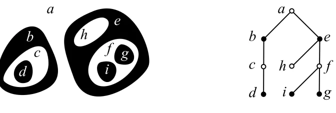
are on fire and not on fire, or they might be land and water. We also assume that any two foreground or any two background regions are disjoint. In the plane this leads to a picture such as that on the left hand side of Figure 1, where the foreground regions are shown black and the background ones white.
a
a
c
h
f
b
e
g
i
d
c
h
f
b
e
g
i
[image:4.612.140.476.194.307.2]d
Figure 1: A system of nested regions in the plane and its adjacency tree
We do not require that regions are parts of a two-dimensional space, but we do assume that the only spatial relationship between regions is nesting. This may seem restrictive, and regions which overlap or have more elaborate relationships are certainly needed in some applications. However as the initial step for the development of the theory our choice is a natural one which is supported by its use by other authors. For example, in Milner’s theory of bigraphs [Mil08] the spatial aspect is restricted to nested entities.
The nested structure leads to an associated tree, which is most easily explained in the planar case, and which is illustrated in Figure 1. In this case we can take the foreground regions to be a compact set K in the plane R2. If we use K0 to denote the closure of the complement of K, then the nodes of the associated tree are the connected components ofK together with the connected components of K0. The root of the tree is the single unbounded component ofK0, and two nodes are adjacent in the tree if they are distinct and have intersecting boundaries. This tree, or its analogue for the digital plane Z2, has been called the adjacency tree [Bun69, Ros74]. In Figure 1 the tree is shown with nodes partitioned into two classes coloured black and white corresponding to the foreground and background regions respectively. This colouring is shown only in order to make the association with the regions in the figure clearer; the trees used in the formal analysis do not come equipped with a particular choice of black or white for each node.
intrinsic reason to prefer one node of the tree above any other. The work by Jiang and Worboys [JW09] used rooted trees, and concentrated on planar regions. Apart from Egenhofer’s spherical topological relations [Ege05], there is relatively little work on qualitative distinctions which can be made on the sphere but not in the plane. Our main result, Theorem 13, is stated in terms of trees which do not have a specified root and thus applies directly to dynamic configurations of regions on the surface of the sphere. However, in deriving this result we sometimes need to single out a node for special treatment, as in the rooted-sums in Section 3.2. When we do need to consider such structures it should be noted that a rooted tree is formally just a pair consisting of a tree together with any one of its nodes.
In mathematical morphology Serra [Ser82, p89] used the term ‘homotopy tree’ instead of adjacency tree, although the same term is used elsewhere for a quite dis-tinct concept [Dye79, p378]. The morphological applications include algorithms for noise removal [Kes07], and for skeletonization [RS02]. In the case of skele-tonization, and several other uses of adjacency trees, the emphasis is on transfor-mations of the image that leave the tree unchanged. That the tree remains fixed is particularly important in applications to visual markers [CR03], where the tree is used as the means of identifying a particular marker in a scene. For our purposes, however, the fact that the tree changes is essential and the ways this may happen are discussed in the next subsection.
1.3
Dynamic aspect
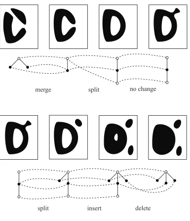
Particularly simple changes are those where the number of regions increases or de-creases by only one. A change is detected by a difference between configurations at two times and our model does not record the process by which the change was brought about. Four kinds of primitive change are immediately evident: insertion (a new region has been created); deletion (an existing region has disappeared); merge (two regions have joined to become one); split (one region has divided into two). The simplest kind of merge in the two-dimensional setting is when two re-gions which are topologically discs unite to become a single region which is again topologically a disc. There are more complex kinds of merging, such as that illus-trated in Figure 2 where two regions have encircled a third. In this case the region that results from the merge is not topologically a disc but has a hole containing another foreground region.
Figure 2: Sequence of changes in which two regions encircle a third
and rectification, which includes the redrawing of a shared boundary between two parcels without affecting their overall extent. There are also two complex changes (‘re-allocation’ and ‘expropriation’). In [JYG03, p931], Jin et al. argue for the ex-plicit modelling of ‘identity changes’ between objects (such as one splitting into two) in order to deal with queries such as ‘Was the objectOmerged into another object in a given time interval?’. Medak [Med99] is also concerned with track-ing identity, and works in a framework where identities may not only be created and destroyed but also suspended and resumed. A distinction is made between fusions, which are irreversible operations like forming one container of liquid out of two, and aggregations, in which constituent parts can still be identified. Robert-son et al. [RNBW07] examine spatial processes, identifying five types of events: displacement, convergence, divergence, fragmentation and concentration. They provide a case study of a wildfire, and the relationships shown diagrammatically in their fig 8 [RNBW07, p223] provides a practical example to which our theoret-ical analysis in this paper is immediately applicable.
Our treatment is based on atomic primitives: insertion, deletion, merge and split where only one region is inserted, is deleted, splits or where just two regions merge. In addition to these four, we also need a fifth primitive for the case of no change being observed. Each of these five atomic changes gives rise to a relation between the nodes of the trees for the initial and final states. By composing se-quences of such changes we obtain more general relations between the adjacency trees. The term ‘relation’ here means nothing more than a set of ordered pairs in the usual mathematical sense. So a relation pairs certain nodes between two trees. The relations that arise by composing the atomic changes are not arbitrary relations on the nodes, but will evidently preserve the partitioning of the nodes in a tree into foreground and background nodes.
con-figuration is something that exists in addition to the states themselves and is not (except in some very special cases) something that can be deduced unambigu-ously from the states themselves. To take a very simple example, consider the initial state of a single background region and a single foreground region. Sup-pose the final state consists of a single background region and two foreground regions. Between these two states are various possibilities including that the ini-tial foreground region has split into two and that a new foreground region has been inserted. Our model assumes that the relation between these states will be given explicitly as part of the information that we work with.
Suppose now that we take two adjacency trees each with a partition of the nodes into those representing foreground regions and those representing back-ground regions. In such a partition any two nodes of the same type must be an even number of edges apart. If we specify an arbitrary relation between the fore-ground nodes and another arbitrary relation between the backfore-ground nodes, these two relations taken together give a single relation between the nodes of the two trees. In the formal analysis below we call relations between trees that have this form bipartite. The main technical result in the paper, Theorem 13, shows that all bipartite relations between trees arise from the composition of atomic primi-tive relations of the five types. This theorem answers a natural question from a theoretical perspective, but the question is also of practical importance. Suppose we have two systems of foreground and background regions, which might for example represent regions occupied by crowds at two times. A bipartite relation between the adjacency trees models how the crowds at the first stage participate in the formation of the crowds at the latter stage. Theorem 13 tells us that every pos-sible relation can be explained in some way as a sequence of primitive changes, or alternatively that the primitive changes are sufficient to generate all possible relations.
1.4
Qualitative change and conceptual neighbourhoods
proper partof a second region (no region can be externally connected to the first without also overlapping the second). It should be noted that a region may consist of several disconnected pieces.
The RCC-8 allows a spatial configuration to be described by giving a set of regions and specifying which of the eight relations holds between each pair of regions. This is a similar approach to that in the static aspect of the model in this paper. In our case there are just two possibilities for each pair of regions; either they are adjacent or they are not. If regions are adjacent then the RCC-8 relation between them will be external connection, and if they are not adjacent then in RCC-8 terms they would be disconnected. A general RCC-8 configuration could be represented by a graph having a node for each region and one edge between every pair of nodes with edges labelled by the eight possible relations. This would be more general than the adjacency trees which we use, but it is in the dynamic aspect that the RCC-8 and our model have taken significantly different approaches.
Many qualitative spatial calculi, including RCC-8, allow a treatment of spatial change through the notion of a conceptual neighbourhood [Fre91]. In the RCC-8 case, two relations S1 and S2 of the eight are said to be conceptual neighbours if a continuous change to a spatial configuration allows the relation between two regions to change from S1 to S2 without passing through any other of the eight relations. The idea of ‘continuous change’ is often used rather informally in this setting, and Galton has shown, [Gal97], that several different definitions are pos-sible so that an appropriate choice will depend on a particular application domain. The kinds of change permitted by the conceptual neighbourhood approach are quite different from those discussed in this paper. This is mainly because the effects of splitting, merging, creating and deleting regions lead to changes in spatial relationships which are not conceptual neighbours. This can be seen from an example. Consider the RCC-8 description of the change observed of two regionsrandswhererconsists of two disconnected piecesr1andr2, wherer1is a non-tangential proper part ofsandr2 is disconnected froms. The relation ofr tosis that they properly overlap. Now ifr2 is deleted the relation betweenrand sbecomes that ris a non-tangential proper part ofs. This transition from proper overlap to non-tangential proper part is not one between conceptual neighbours in the RCC-8.
to record the sequence of changes that the relation between each pair of regions undergoes. If the initial and final states were each modelled by a graph with nodes corresponding to regions and labelled edges corresponding to spatial relations, then such a sequence of changes would relate edges to edges. This would be quite different from our use of a relation between the sets of nodes.
1.5
Overview
The structure of the paper is as follows. Section 2 defines various types of relations between trees, the most important of which are the bipartite relations. Section 3 sets out constructions we need which enable trees and relations to be built up out of simpler components. The bipartite relations include the atomic relations which model primitive changes and these are defined in Section 4. This section also introduces what we call the evolutions, which model changes to adjacency trees that can be accomplished by a sequence of successive atomic changes.
The main technicalities in the paper appear in sections 5 and 6, where we study relations between chains which are very simple trees. We show how the issue of whether all bipartite relations between arbitrary trees are evolutions can be reduced to a question about relations between chains. Section 7 contains the main result, showing that bipartite relations are the same as evolutions. This re-sult, Theorem 13, shows that any bipartite relation can be factorized into atomic relations, and the connections with another factorization result, obtained by Jiang and Worboys [JW09], are explained in Section 8. Finally in Section 9 we present some conclusions and suggestions for further work.
2
Relations between trees
In this section we introduce the basic definitions of trees and of relations between trees. Although the motivation for the theory is the description of qualitative spatio-temporal change, the formal development is entirely in terms of structures on trees. We use some informal examples of evolving spatial regions, but our re-sults only concern such regions to the extent that their properties are modelled by adjacency trees, and their transitions are modelled by relations.
2.1
Relations, graphs and trees
Given sets X, Y, Z and relations R1 : X → Y andR2 : Y → Z we adopt the notationR1;R2for the composition ofR1andR2as used, for example, in [HH02, p3]. The relationR1;R2 is defined byx (R1;R2)z iff there is somey ∈ Y for whichx R1 yandy R2 z.
The converse of a relation R will be denotedR−1. By a subrelation of R : X → Y we will mean any relation S : X → Y for whichx S yimpliesx R y. The notationS ⊆ R will be used in this case. Given a relationR : X → Y and a subset A ⊆ X we will useR(A)to denote {y ∈ Y | ∃a ∈ A (a R y)}. We say thatRis functional ifx R yandx R zimplyy= z. A functional relation is sometimes called a partial function. The term function, used without qualification, will be assumed to be a total function.
Definition 1. Agraph,G, is a pair(N, α)whereN is a set andαis a symmetric relation on N. The elements ofN are called thenodesof Gandα is called the
adjacency relationofG. AnedgeofGis a pair of nodes(m, n) ∈ N ×N such thatm α n. Thedegreeof a node is the number of nodes to which it is adjacent.
Trees, which we define shortly, are graphs of a particular form, but we also need to consider a larger class of graphs which includes the trees.
Definition 2. Abipartite graphis a graph,G = (N, α), whereN can be written asN =N1∪N2 such thatN1∩N2 =∅andα⊆(N1×N2)∪(N2×N1).
In a bipartite graph the nodes can be partitioned into two disjoint sets and every pair of nodes forming an edge will have exactly one element from each of these two sets. The significance of bipartite graphs for our application to spatial configurations is that regions will correspond to nodes in a graph, and the division into foreground and background regions is then modelled by the partition of the nodes into disjoint sets where adjacent nodes must come from different sets in this partition.
Definition 3. Atree, T, is a graph(N, α)such that given any nodes m, n ∈ N there is a unique sequence of nodes n0, n1, . . . , nk wherem = n0, n = nk, and
ni−1 α ni fori = 1, . . . , k. This sequence of nodes is called thepathbetweenm andn. AsubtreeofT is a subset ofN which is a tree when the adjacency relation is restricted to this subset.
Definition 4. Arooted treeis a pair(T, r)whereT is a tree andris a node ofT.
Since our trees are undirected graphs the root of a rooted tree has no special status with respect to the tree regarded as an abstract structure on its own. That is, we may consider the same tree but with different roots at different stages in a construction. When it is necessary to change the root of a rooted tree, we will say that the structure has been ‘re-rooted’.
In a treeT = (N, α)we can define a relation∼onN by m ∼ n if the path betweenmandncontains an odd number of nodes. The relation thus defined can also be described by saying thatmandnare related if they are an even number of edges apart. It can be checked that∼is an equivalence relation and that there are two equivalence classes which partitionN into disjoint subsets makingT a bipar-tite graph. We will use the notation[m]when we need to refer to the equivalence class of the nodem.
2.2
Homomorphisms and bipartite relations
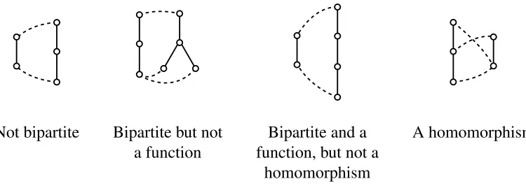
It will be assumed below thatT1 = (N1, α1)andT2 = (N2, α2)are trees. We will speak of a relation,R, between trees whenever we have a relation between the sets of underlying nodesR :N1 →N2. We need to consider various kinds of relation, and some representative examples are shown in Figure 3. In this and subsequent figures we indicate the relation by dashed lines and the adjacency in the trees by solid lines.
Not bipartite Bipartite but not Bipartite and a A homomorphism a function function, but not a
[image:11.612.121.496.459.592.2]homomorphism
Figure 3: Examples of types of relations between trees
Definition 5. Ahomomorphism f : T1 → T2 is a function from N1 to N2 such
The inverse of a bijective homomorphism between trees will again be a homo-morphism, so we can define anisomorphismto be a homomorphism of this form. A homomorphism is a structure preserving function, where the preserved struc-ture is the adjacency relation. The natural generalization to strucstruc-ture preserving relations is as follows.
Definition 6. LetR : T1 → T2 be a relation and letm1, n1 ∈ N1 andm2, n2 ∈ N2. We say thatRpreserves adjacencyif
m1 R m2andn1 R n2 andm1 α1 n1 impliesm2 α2 n2.
It is evident from Figure 4 that we need to deal with relations that are more general than the adjacency preserving ones. For the relation, R, depicted in Fig-ure 4, we have thatbandcare adjacent, butb R dandc R cwheredandcare not adjacent.
To avoid potential confusion, we should point out that although Figure 4 uses the labels a, b, c for nodes in the source tree as well as in the target tree for the relation, this has no particular significance in the formal model. That is, any connection that exists between nodes in the two trees is only modelled by the relation between the trees and not by some of the nodes being equal. In this particular example we could replace either tree by an isomorphic one without affecting the way the relation models three regions where one splits into two.
To introduce the kind of relations we deal with, note that in any tree we have a notion of distance between nodes by counting the number of edges in the unique path joining any two nodes. Given nodes m, n we will denote this distance by d(m, n). If the relation R preserves adjacency, then it is not hard to see that it need not preserve distance in general. However it will preserve distance mod 2, that is whether the distance is odd or even. This can be readily shown by induction on the distance between any two nodes.
The class of relations that preserve distance mod2 are strictly more general than the adjacency preserving ones. We call these relationsbipartite, for reasons that we establish after the definition.
Definition 7. A relationR : T1 → T2 isbipartiteif for allm1, n1 ∈ N1 and for
allm2, n2 ∈N2
m1 R m2 andn1 R n2impliesd(m1, n1)≡d(m2, n2) (mod 2).
a
c
b
a
c
b
d
a
c
b
d
a
b
c
Figure 4: Showing the need for relations which do not preserve adjacency
Lemma 1. A relationR : T1 →T2 is bipartite if and only if for allm1, n1 ∈ N1
and all m2, n2 ∈ N2 where m1 R m2 and n1 R n2, we have [m1] = [n1] iff [m2] = [n2].
The lemma shows that to specify a bipartite relation it is sufficient to choose one equivalence class in each tree and to give an arbitrary relation between these classes and to give an arbitrary relation between the other two equivalence classes. In terms of our spatial interpretation, this means that if we give an arbitrary rela-tion between the sets of foreground regions at two stages and another arbitrary relation between the sets of background regions at the same two stages then we have a bipartite relation between the adjacency trees. Thus every change in the regions can be modelled by a bipartite relation. The converse issue of whether every bipartite relation can arise from splitting, merging, inserting and deleting of regions is not so easily answered but Theorem 13 shows that this does happen.
As with the adjacency preserving relations, the bipartite relations are closed under composition, and include the identity relations. Unlike the adjacency pre-serving relations, the bipartite relations are also closed under the formation of converses. We record these facts as a lemma.
Lemma 2. The identity relation on any tree is bipartite. The composite of bipartite relations is bipartite, and the converse of a bipartite relation is bipartite.
When dealing with rooted trees, (T1, r1) and (T2, r2), we may need to use relations which respect this additional structure as follows.
Definition 8. A rooted homomorphism f : (T1, r1) → (T2, r2) is a
homomor-phism for whichf r1 =r2. Arooted bipartite relationR : (T1, r1)→(T2, r2)is a
bipartite relation wherer1 R r2.
Tree with one Tree with two nodes node distinguished. and one edge distinguished
Figure 5: Components of structure diagrams
3
Constructions on trees and relations
Relations can be built up by composition, and this corresponds in our application to the succession of changes in time. In this section we introduce further means of constructing more complex trees and relations from simpler ones. The notion of rooted sums can be used to model the combination of changes to entities taking place in separate parts of some larger background.
3.1
Structure diagrams
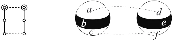
We first introduce a diagrammatic notation for describing relations between trees. We frequently need to deal with relationsR:T1 →T2 where for some subtreeS1 ofT1 the relationR restricts to an isomorphism betweenS1 and a subtree ofT2. By specifying such isomorphisms for a family of subtrees which together cover all of T1 we may be able to describe the whole relation. The resulting diagrams will be found practically useful in describing constructions and explaining proofs later in the paper.
Figure 6: Example of a structure diagram and a relation having this structure
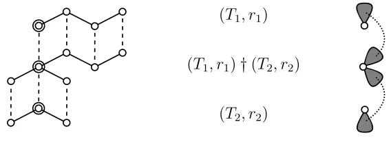
(T1, r1)
(T1, r1)†(T2, r2)
(T2, r2)
Figure 7: The rooted sum of two rooted trees and associated diagram.
3.2
Rooted sums
The idea of the rooted sum of two trees, T1 and T2, is that a node is specified in each tree and we form a new tree by gluing copies of T1 and T2 together at the specified nodes. An example is shown in Figure 7. In this and subsequent figures the specified node (i.e. the root) of a tree is indicated by an extra circle around the node.
Definition 9. Let(T1, r1)and(T2, r2)be rooted trees. Their rooted sum,(T1, r1)† (T2, r2), has the set of nodes((N1−{r1})×{1})∪((N2−{r2})×{2})∪{0}. The
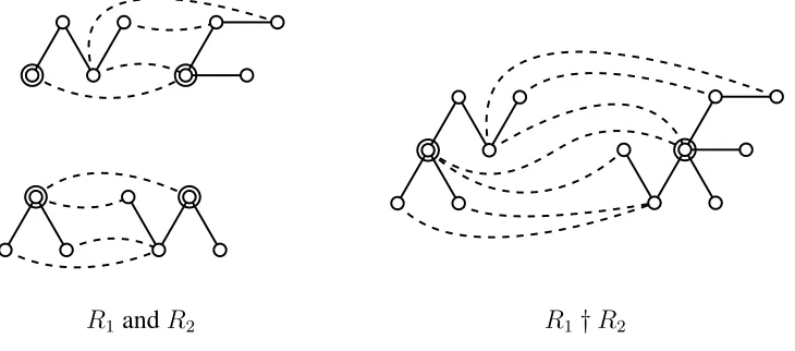
[image:15.612.164.448.321.426.2]R1 andR2 R1†R2
Figure 8: The rooted sum of two rooted bipartite relations.
satisfies the following conditions.
0 (α1†α2) (m,1) iff r1 α1 m, 0 (α1†α2) (m,2) iff r2 α2 m, (m,1) (α1†α2) (n,1) iff m α1 n, (m,2) (α1†α2) (n,2) iff m α2 n.
This construction may be extended from rooted trees to rooted bipartite rela-tions.
Definition 10. Given rooted bipartite relations Ri : (Ti, ri) → (Ti0, ri0) for i =
1,2, their rooted sum R1 †R2 : ((T1, r1)† (T2, r2)) → ((T10, r 0 1)† (T
0 2, r
0 2)) is
defined to be the relation wherex(R1†R2)yiff
x= 0andy= 0, or
x= (m,1), y = (n,1), andm R1 nfor somem ∈N1, n∈N10, or x= (m,2), y = (n,2), andm R2 nfor somem ∈N2, n∈N20.
An example of the rooted sum of relations is shown in Figure 8. It is straight-forward to check that the rooted sum of rooted bipartite relations is again bipartite.
4
Atomic relations
relations by composition. These five types may thus be considered atomic com-ponents out of which all other bipartite relations may be constructed. The moti-vation for the choice of these particular atomic relations comes from our intended application to qualitative changes to regions on the plane or the sphere.
4.1
Examples of atomic relations
The five types of atomic relation we consider are: merge, split, insert, delete, and no change. These are illustrated in Figure 9 which shows a sequence of changes to planar regions above the corresponding sequence of relations between each pair of successive trees. In this figure the nodes of the trees are coloured black or white to indicate whether they correspond to foreground or background regions respectively. As with Figure 1, this colouring is for illustrative purposes only and is not part of the formal structure being considered.
There are two instances of a split in Figure 9. In the first the single black re-gion encloses a portion of the white background rere-gion, splitting the white rere-gion into two. In the second, the black foreground region grows a subsidiary part which then breaks off. Jiang and Worboys [JW09] refer to a ‘self merge’ when the back-ground splits and use ‘split’ for the foreback-ground case. These two cases can only be distinguished in the abstract model if the trees we deal with are equipped with some additional structure which specifies which nodes correspond to foreground regions and which to background ones. In the present paper we do not include such additional structure, and thus we do not distinguish different kinds of splits or different kinds of merges.
4.2
Atomic relations: Diagrams and definitions
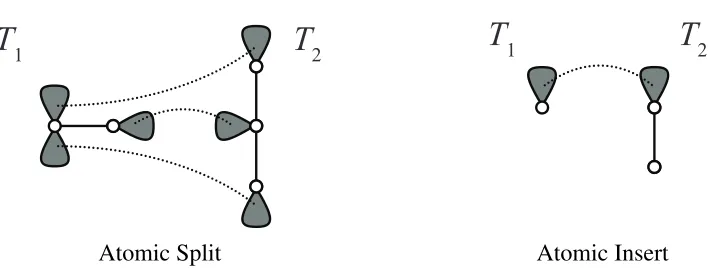
Definition 11. Anatomic splitfromT1 toT2 and anatomic insertfromT1 toT2
are bipartite relations having the forms shown in Figure 10. An atomic merge
fromT1 toT2 is a relation the converse of which is an atomic split fromT2toT1.
An atomic delete from T1 to T2 is a relation the converse of which is an atomic
insert fromT2 toT1. Anatomic relationis any relation of these four forms or an
isomorphism.
merge
split
split
insert
delete
[image:18.612.116.501.161.608.2]no change
T
1T
2T
1T
2 [image:19.612.128.482.118.252.2]Atomic Split Atomic Insert
Figure 10: Atomic relations (see Definition 11).
cannot be inserted or deleted. Note that if two trees are related by an atomic relation then the number of nodes differs by at most one.
Although atomic relations are the focus of our approach, it may be argued that these fail to model all possible changes to regions because there might be simul-taneous merging or splitting. For example, in Figure 2 the two encircling regions might join together in two places at the same time. This is clearly a physical possi-bility that could be important in some applications. In this particular example the capture of the central region by the two outermost ones can readily be expressed as the composite of two atomic relations. Should it be necessary to capture a notion of concurrency then an appropriate equivalence relation on sequences of atomic relations could be introduced.
4.3
Evolutions
By composing atomic relations we can generate more complex relations.
Definition 12. Anevolutionbetween trees is any relation that arises from compos-ing a sequence of atomic relations. Similarly, arooted evolutionbetween rooted trees is a rooted relation obtained by composing atomic rooted relations.
As the atomic relations are bipartite, the evolutions are bipartite by Lemma 2. The evolutions are clearly closed under composition and under taking converses and they include all isomorphisms. We will also need the fact that they are closed under rooted sums. If R : (T1, r1) → (T10, r
0
Lemma 3. LetR : (T1, r1)→(T10, r 0
1)be a rooted evolution, letI be the identity
relation on (T2, r2). Then R †I : (T1, r1)†(T2, r2) → (T10, r10)†(T2, r2)is an
evolution.
Corollary 4. LetRi : (Ti, ri) → (Ti0, r
0
i)be rooted evolutions fori = 1,2. Then
R1†R2 is a rooted evolution.
Proof. We can writeR1†R2 = (R1†I2) ; (I10 †R2) = (I1†R2) ; (R1†I20), where theIi andIi0denote the identity relations on the treesTiandTi0respectively.
5
Chains and ladders
In this section we consider trees of a particularly simple kind in which the nodes with their adjacency relation constitute a linearly ordered set, also called a chain.
5.1
Definitions and examples
Definition 13. The tree with nodes {1, . . . , n} where n > 1 and adjacency α wherei α i+ 1will be denotedn. Any tree isomorphic to somenwill be called a
chain. A chain in which one of the nodes of degree 1 is distinguished as the root will be called adirected chain.
Definition 14. Aladderis any relation which is isomorphic to a subrelation of the identity relation on a chain.
Relations which are ladders can be drawn (see Figure 11) so that the only nodes which may be related are those which align horizontally. Not every pair of horizontally aligned nodes need be related so the effect is of a ladder in which some of the rungs may be missing. If no rungs are missing then the ladder is an isomorphism between chains.
Definition 15. Adirected ladderis any relation which is isomorphic to a subre-lation of the identity resubre-lation on a directed chain.
Note that there is no requirement that a directed ladder should be a rooted relation. That is, the two root nodes on the two chains forming the two sides of the relation need not be related.
1 2 3 4
[image:21.612.151.469.112.241.2]The chain4 The directed ladders Composing1101 1101and0111 and0111gives0101.
Figure 11: Examples of ladders
thati λ i, and a 0 indicates that this is not the case. Figure 11 provides examples. If λ = λ1λ2· · ·λn and µ = µ1µ2· · ·µn are both ladders of length n then the
composite is given byλ;µ= (λ1∧µ1)(λ2∧µ2)· · ·(λn∧µn), whereλi∧µiis0
unless bothλiandµi are1. This operation on sequences is known [Knu98, p111]
as thebitwise andof the sequences.
[image:21.612.157.452.463.539.2]5.2
All ladders are evolutions
Figure 12 shows the directed ladder101, which is the simplest case where it is not immediately obvious how to express the directed ladder as a composite of atomic relations.
a
b
e
c
d
f
Figure 12: The directed ladder101and a possible interpretation.
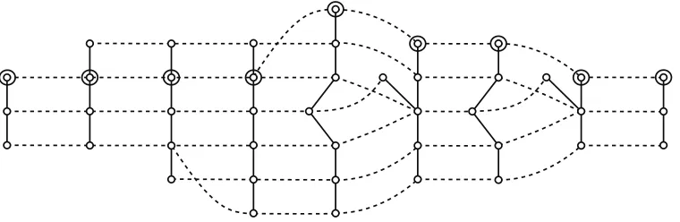
Figure 13: The directed ladder101as a composite of eight atomic relations.
To visualize a possible interpretation, imagine the surface of the sphere cov-ered by lakes of two types of substance coloured black and white. The entity labelledain the figure should be understood as a quantity of white material rather than the part of the surface of the sphere that this material occupies. The atomic relations available to us mean that lakes of opposing colours cannot merge with each other, but two lakes of the same colour may combine to form a single lake. The properties of composition of relations imply that once two lakes of the same colour have merged they cannot be separated again. This is because if lakesxand ymerge intozwe would havex R zandy R zfor some relationR. Then for any relationSwe will havex(R;S)wiffy(R;S)w.
As the atomic relations include inserts and deletes, new disc-like lakes may appear within lakes of the opposite colour, and lakes may disappear provided they have just a one-piece boundary. The black equatorial band has a two-piece boundary and thus cannot disappear without the two white lakes a and c first merging with each other. This means, in particular, that to obtain the ladder 101 as a composite of atomic relations we require something more complex than the deletion ofbfollowed by the insertion ofe.
d. Consideration of the properties of the operation of composing relations shows that the exclusive link does not exclude the possibility that parts of a may have split off, then merged with parts of c, and then been deleted. Additionally, we cannot infer from this exclusive link that the lakedcontains material only present ina. This is because a new lake might have been created between the initial and final stages and this new region might have merged with the region that becamed.
Lemma 5. The directed ladder101is an evolution.
Proof. A factorization into atomic relations is provided in Figure 13. The eight atomic relations are: insert; insert; split; split; merge; delete; merge; delete.
We can use the idea of rooted sums of relations to show that ladders can always be expressed as sequences of atomic relations.
Theorem 6. Every ladder is an evolution.
Proof. Given an arbitrary ladder λ, we can choose a direction and assume we have a directed ladder. We have noted that directed ladders correspond to binary sequences and that the composition of relations corresponds to taking the bitwise
andof such sequences.
Now every binary sequence is expressible as the bitwiseand of a number of sequences each of which contains at most one zero. Thus the result follows if we can show that every ladder with exactly one rung missing is an evolution.
If the missing rung is the top or bottom one, a delete followed by an insert gives us what we require. If the missing rung is in the i-th place in a ladder of length n and1 < i < nthen we use Lemmas 5 and 3 as follows. The directed ladder, Λ, of length i+ 1 which lacks only the second rung can be obtained by re-rootingI †101 whereI is the identity relation on the chaini−1. The ladder we require is then obtained from Λ †J, where J is the identity relation on the chainn−i.
6
Relations between chains
p
2p
1p
0p
n 1p
np
n+1q
s
2s
1s
dp
2p
1p
0p
n 1p
np
n+1q
s
2s
1s
dr
1r
2r
n 1 [image:24.612.138.475.107.365.2]r
nFigure 14: Construction in proof of Lemma 7
between chains. We have already met some simple relations between chains in the ladder relations, and these were all shown to be evolutions in Theorem 6. This section generalizes this result to show in Theorem 12 that all bipartite relations between chains are evolutions.
6.1
Reduction to chains
First, we recall an observation about ordinary relations. If α : A → B is any relation between sets A and B, and α is injective and total then α;α−1 = I, whereα−1is the converse ofα, andIis the identity relation onA. This is because αis total iffI ⊆α;α−1, andαis injective iffα;α−1 ⊆I.
Lemma 7. For any tree,T, there is a chainCand an evolutionα:T →C which is injective and total.
Proof. The relationαis constructed as the composite of a sequence of evolutions αi :Ti−1 →Ti fori= 1, . . . , m, and whereT =T0 andTm =C.
Assume inductively that we have constructedαi :Ti−1 →Ti fori= 1, . . . , k,
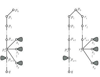
it is a chain, and we are done. If there are more than two nodes of degree one, then let p0 andq be any two distinct such nodes in Tk. Consider the path from
p0 toq. This will have an initial segment of the formp0, p1, . . . , pn, pn+1 where pj has degree two for j = 1, . . . , n−1, andpnhas degree strictly greater than2.
Let the nodes adjacent topnbe{pn−1, pn+1, s1, s2, . . . , sd}. The treeTk+1has the same nodes as Tk together with n new nodesr1, r2, . . . , rn attached as shown in
Figure 14.
The relation αk+1 : Tk → Tk+1 is the union of the identity relation on the nodes of Tk with the relation pj αk rj forj = 1, . . . , n. Clearly this is injective
and total. It is easily checked that αk+1 is an evolution by using a sequence of splits at each of pn, pn−1, . . . , p1 to obtainTk+1 fromTk. SinceTk+1 has exactly one fewer node of degree one thanTk, (i.e.p0 in the above construction) we must eventually obtain a chain.
From the lemma we obtain the following result which shows that if every bipartite relation between chains is an evolution, then every bipartite relation be-tween arbitrary trees is an evolution.
Corollary 8. Any bipartite relationR :T1 →T2 can be expressed asα;R0;β−1
whereR0is a bipartite relation between chains, and whereαandβare evolutions as in the diagram with α ; α−1 and β ; β−1 being the identities on T1 and T2
respectively.
T1
α
> C1
α−1 > T1
T2 R
∨
< β −1
C2 R0
∨
< β T2 R
∨
Proof. Construct α : T1 → C1 and β : T2 → C2 as the injective and total evolutions from the two trees to chains by the method in Lemma 7. The relation R0is defined to be the compositeα−1;R;β, and the above diagram commutes.
6.2
Tangled pairings
When dealing with relations between trees where the source and target are the same we can distinguish two kinds of bipartite relations.
Definition 16. LetR : T → T be a bipartite relation. We say R is directif for all nodesx, y, we havex R y implies[x] = [y]. IfR is not direct, it is said to be
reverse.
IfRis a direct bipartite relation andx R ythen the distanced(x, y), as defined in Section 2.2, will be even. If Ris reverse then this distance will be odd. Some examples of direct and reverse bipartite relations appear in Figure 15.
1
2
3
4
1
2
3
4
1
2
3
4
1
2
3
4
Reverse bipartite relations. The right hand one is a permutation of{1,2,3,4}.
1
2
3
4
1
2
3
4
1
2
3
4
1
2
3
4
Direct bipartite relations. The right hand one is
[image:26.612.121.498.298.439.2]a tangled pairing.
Figure 15: Examples of direct and reverse bipartite relations on the chain4
Definition 17. A tangled pairing on a chain C is any direct bipartite relation R :C→C which is a bijective total function on the set of nodes inC.
Atransposition on a chainC is any tangled pairing R : C → C for which there are exactly two nodesnsuch thatn R ndoes not hold.
A tangled pairing is thus a permutation on the set of nodes. We will use (n1, n2) to denote the transposition that swaps nodes n1 and n2 while leaving all others fixed. Since transpositions are direct bipartite relations the two nodes that are transposed must be an even number of edges apart in the chain.
Proof. Let the two equivalence classes inC beK1 andK2. The setsK1 ∩(C− R−1(C))andK1∩(C−R(C))have equal numbers of members, and the same is true ofK2∩(C−R−1(C))andK2∩(C−R(C)). So we formR0 by bijectively pairing, in any way, elements ofK1∩(C−R−1(C))with elements ofK1∩(C− R(C)), and elements ofK2∩(C−R−1(C))with elements ofK2∩(C−R(C)).
Lemma 10. Every tangled pairing is an evolution.
Proof. First we show that all transpositions are evolutions. We have seen in The-orem 6 that all ladders are evolutions. Combining this result with Lemma 3, we know that the relationR2shown in Figure 16 is an evolution. The relationsR1and R3in this figure are also evolutions, being respectively two splits and two merges. Hence the compositeR1;R2;R3, that is the transposition(2,4)on the chain5, is an evolution.
[image:27.612.123.483.334.449.2]R1 R2 R3 (2,4)
Figure 16: ComposingR1,R2andR3 gives the transposition(2,4).
Knowing that the transposition (2,4)is an evolution, we see (making use of Lemma 3) that all transpositions in which the two transposed nodes are exactly two edges apart are also evolutions. That is, if we number the nodes in the chain n0, n1, . . . , nkthen we can obtain every transposition of the form(ni, ni+2). From this we get that all transpositions are evolutions, since letting π = (ni, ni+2) ; (ni+2, ni+4) ;· · ·; (ni+2j−4, ni+2j−2)we can express an arbitrary transposition as (ni, ni+2j) = π; (ni+2j−2, ni+2j) ;π−1.
6.3
Arbitrary relations between chains
We can now demonstrate that all bipartite relations between chains are evolutions. This result is Theorem 12 below, before which we need a lemma. Note that the lemma includes the case of permutations of the nodes of a chain which are reverse bipartite relations and thus not covered by Lemma 10 above.
Lemma 11. If R : C → D is an injective and functional bipartite relation be-tween chains thenRis an evolution.
Proof. Suppose thatC andDhavem andn nodes respectively. We can assume that C and D are the chains m and n. The proof proceeds by writing R as a compositeR1;R2 ;R3 whereR2is a tangled pairing andR1 andR3have simple forms which are evidently evolutions. The relation R2 will be constructed by extending another relationS.
Letibe the least element ofmfor which there is aj such thati R j. AsRis functional, thisjis unique. We now consider two cases according asi>j or not. Wheni>j, take`to be the maximum ofmandn+i−jand defineS :` →` byx S yiffx R (y−i+j). DefineR1 :m→`byR1 ={(x, x)| ∃y(x R y)}, and defineR3 :` →nbyR3 ={(x, x−i+j)|x=i−j+ 1,· · · , i−j+n}.
When i < j, define ` to be the maximum of n and m +j −i and define S :`→`byx S y iff(x+i−j)R y. We defineR1 :m→`by
R1 ={(x, x+j−i)| ∃y(x R y)},
and we defineR3 :`→nbyR3 ={(x, x)|x= 1,· · · , n}.
In each caseSis bipartite and is injective and functional sinceRis, buti S i soSis a direct bipartite relation. Thus by Lemma 9 we can extendSto a tangled pairingR2on`. We have thus expressedRas a composite of three evolutions.
Theorem 12. Any bipartite relationR :C→Dbetween chains is an evolution.
Proof. The technique is to writeR=Rinj;Rfnl, whereRinjis injective andRfnlis
functional.
Letz ∈Dbe any node for whichx R zandy R zfor distinctxandy. Make a new chain from D by replacing the nodez by a chain the nodes of which are pairs
(x1, z),(w1, z),(x2, z),(w2, z), . . . ,(wn−1, z),(xn, z)
where x1, w1, . . . , xn is the interval in C with endpoints the extreme elementsx
for which x R z (i.e. any xsuch that x R z lies in the interval from x1 toxn).
Now letR0 : C → K act as R except that whenever x R z we now have x R0 (x, z) and, in general, x R0 (x0, z) iff x = x0 and x R z. We can also define R00 : K → Dby a R00 b iff a = b ora = (xi, b) for somexi. We then
have R = R0 ;R00 and by repeating this process on R0 we will eventually arrive at a stage where R0 is injective and the composition of all the R00s provides the required functional relation Rfnl. We can see that each R00 is an evolution as it
arises by merging all the(xi, z)with each other, and deleting the node that results
from merging together all the(wi, z)with each other. We will need the fact that in
this construction ifRis functional thenRinjwill be functional as well as injective.
We have factorized R into an injective part, Rinj, and a functional part,Rfnl.
The functional part has been shown to be an evolution so we are left with an arbitrary injective bipartite relation to deal with.
Consider the converse of this relationRinj−1. By applying the above process
to this relation, we arrive at Rinj−1 = S1 ; S2 where S1 is injective and S2 is an evolution. Since Rinj−1 is functional we have that S1 is both injective and functional. The result then follows from Lemma 11.
7
The characterization of evolutions
The main result now follows from Theorem 12 and Corollary 8.
Theorem 13. For any two trees T1, T2, the evolutions fromT1 toT2 are exactly
the bipartite relations fromT1 toT2.
Relations between abstract trees (without any additional structure, such as a choice of root) correspond most naturally to bounded regions evolving on a sphere, such as the surface of the Earth. For some applications, however, it can be more natural to consider bounded regions evolving against an unbounded plane background. This is the case examined in [JW09] and corresponds to using rooted trees because the background has a special status. The background may not be deleted, although it may be involved in splitting and merging. We can use our result Theorem 13 to show that the analogous statement holds in the rooted case.
Corollary 14. For any two rooted trees(T1, r1), (T2, r2), the rooted evolutions
Proof. Suppose we are given a rooted bipartite relationR : (T1, r1) → (T2, r2). By Theorem 13 we can express this as a sequence of atomic relations.
T1 =S1 R1
> S2
R2
> S3 · · · Sn−1
Rk−1
> Sk=T2. Since the relation R preserves the root (i.e. r1 R r2) we can identify a node ni
in each Si for i = 2, . . . , k −1such thatr1 R1 n2 R2 n3· · ·nk−1 Rk−1 r2. By designating these nodes as the roots we make eachRiinto a rooted atomic relation
and so have thatRis a rooted evolution.
8
Fourfold factorizations
We have shown that arbitrary bipartite relations can always be factorized into atomic relations. Previous work by Jiang and Worboys [JW09] deals with a dif-ferent kind of factorization. In this section we show how the two approaches are related.
8.1
Homomorphic relations
So far we have introduced atomic relations and the more general bipartite rela-tions. In order to understand how our approach relates to the results in [JW09] we need to introduce further kinds of relations.
Definition 18. A homomorphic insert is a relation between trees f : T1 → T2
which is an injective homomorphism. A homomorphic delete is a relation the converse of which is a homomorphic insert.
A homomorphic merge is a relation between trees f : T1 → T2 which is
a surjective homomorphism. A homomorphic split is a relation the converse of which is a homomorphic merge.
Any relation of one of the above four forms which is not an isomorphism will be callednon-degenerate.
Lemma 15. The non-degenerate homomorphic inserts are exactly the composites of atomic inserts.
Proof. Composing atomic inserts clearly gives a homomorphic insert. Conversely, letf :T1 →T2 be a non-degenerate homomorphic insert. There must be a node n inT2 of degree 1 which is not in the image off, because if two distinct nodes are in the imagef then every node on the path between them is too. LetT20 be the treeT2with nodenremoved, andα:T20 →T2the atomic insert which inserts this node. We can write f asf0;αwheref0 is a homomorphic insert with one fewer node inserted thanf, so the result follows by induction.
Corollary 16. The non-degenerate homomorphic deletes are exactly the compos-ites of atomic deletes.
Lemma 17. A relationf : T1 → T2 is a non-degenerate homomorphic merge if
and only if it is a composite of one or more atomic merges.
Proof. Composites of atomic merges are clearly homomorphic merges. For the converse, we use induction on the number of sets of nodes{a, b}inT1 which are distance 2 apart and wheref a=f b. If there are no such sets of nodes thenfmust be an isomorphism. LetT10 be the tree with nodes(N1− {a, b})∪ {t}, wheretis a new node not inN1. The nodetis adjacent in T10 to those nodes ofT1 adjacent to at least one ofaandb. Other nodes ofT10 are adjacent to each other as they are inT1. Now letα : T1 → T10 be the atomic relation which merges aandbwitht. We can then writef =α;f0 withf0x=f xwheneverx6=t, andf0t=f a.
Corollary 18. The non-degenerate homomorphic splits are exactly the composites of atomic splits.
The following theorem is a slight reformulation of a result established in [JW09].
Theorem 19(Jiang and Worboys). Suppose the rooted bipartite relationR :T1 → T2between rooted trees is a composite of an arbitrary sequence of relations each
one of which is a homomorphic insert, a homomorphic delete, a homomorphic merge or a homomorphic split. Then R can be expressed as a composite of just four homomorphic relations
T1
RI
> U RS > V RM > W RD > T2
From Lemmas 15 and 17 and Corollaries 16 and 18, it follows by using Corol-lary 14 that the relations R of the form described in Theorem 19 comprise all possible rooted bipartite relations. So we deduce that all rooted bipartite relations admit such fourfold factorizations.
In the remainder of this section we investigate related factorizations in our framework. To start with, we need to recall some basic properties of relations between sets rather than trees.
8.2
Factorizing relations between sets
For a relation R from setX to set Y, there are four especially simple kinds of relation which we can identify.
Definition 19. For a relationR:X →Y with converseR−1 :Y →X,
Ris inserting deleting splitting merging iff
RandR−1are injective, andR−1 is surjective RandR−1 are injective, andRis surjective RandR−1 are surjective, andRis injective RandR−1are surjective, andR−1 is injective
A relation of any one of these forms is called abasic relation.
Note thatRis inserting iffR−1 is deleting, andRis splitting iffR−1 is merg-ing. The following result can probably be described as well-known folklore, but we have included a detailed proof because we need to understand how it extends to trees.
Lemma 20. Any relation R : X → Y between sets admits a factorization into basic relations
X RI > A RS > B RM > C RD > Y
in whichRI, RS, RM, andRD are respectively inserting, splitting, merging, and deleting.
Proof. Assume thatX andY are disjoint, since if not we can find a relation iso-morphic to Rin which they are. DefineEX = {x ∈ X | @y ∈ Y ·x R y}and
EY = {y ∈ Y | @x ∈ X ·x R y}. The required factorization comes from the following diagram of sets and functions
X ι> X∪EY <
σ
EX ∪R∪EY
µ
> EX ∪Y <
whereRis the given relation as a set of ordered pairs. The functionsιandδare the evident inclusions; these giveRI =ι, which is inserting, andRD =δ−1, which is
deleting. The functionσacts as the identity onEX ∪EY and sends(x, y)∈Rto
x. The functionµalso acts as the identity onEX ∪EY, but sends(x, y)∈Rtoy.
These provideRS =σ−1 which is splitting, andRM =µwhich is merging.
It is sufficient to check thatιandµare inserting and merging in order to justify that the four relations RI, RS, RM andRD have the required properties. This is
because the inserting component of R is the deleting component of R−1, that is RI = (R−1)D, and alsoRM = (R−1)S. It is also easily checked that the composite
RI;RS;RM;RD yields the original relationR.
8.3
Factorizing relations between trees
We return now to bipartite relations between trees. The terminology of Defini-tion 19 can be applied directly to these relaDefini-tions.
Suppose R : T1 → T2 is a bipartite relation. It is possible to colour each tree so that every node is either black or white and so that any pair of nodes related byRboth have the same colour. We can express this colouring by writing N1 = B1 ∪ W1 and N2 = B2 ∪W2, where Bi is the set of black nodes for
i = 1,2, andWi is the set of white nodes. Then the bipartite relationR fromT1 to T2 is equivalent to two ordinary relations between setsRB : B1 → B2, and RW : W1 → W2. Note thatRis an inserting if and only if bothRB andRW are
both insertings, and similarly for the other types.
Now,RBandRW each admits a factorization as in Lemma 20 and taking the
unions of the corresponding parts yields a factorization ofR. That is, the inserting component of R is the union of the inserting components ofRB andRW etc. If
a set is partitioned into two then the two subsets can form the two differently coloured sets of nodes of a tree except when one set is empty and the other has at least two elements. Because our T1 and T2 are trees to start with, and from the properties of basic relations, it follows that the factorization obtained for R between the sets of nodes allows all the intermediate sets to be made into trees in a way respecting the colours. Thus we have established the following.
Theorem 21. Any bipartite relationR :T1 →T2admits a factorization into basic
relations
T1
RI
in whichRI, RS, RM, andRD are respectively inserting, splitting, merging, and deleting.
The rooted case is easily obtained from this. IfT1 andT2 have specified root nodesn1, n2 andn1 R n2 then it will be possible to identify a root node in each ofU,V, andW so that the four basic components are rooted bipartite relations.
Corollary 22. Any rooted bipartite relation R : (T1, n1) → (T2, n2) admits a
factorization into rooted basic relations
(T1, n1) RI
>(U, u) RS>(V, v) RM>(W, w) RD>(T2, n2)
in whichRI, RS, RM, andRD are respectively inserting, splitting, merging, and deleting.
The interest of these results lies in the way they depend only on the corre-sponding result for relations between sets. They are however weaker than The-orem 19 because the basic relations need not be homomorphic. Also it should be noted that this theorem does not subsume our main result, Theorem 13, as it would be necessary to show that the four components it includes are themselves sequences of atomic relations.
9
Conclusions and further work
We have shown that evolutions, or composites of atomic relations, are the same as bipartite relations between trees. The motivation for studying such relations is that if we interpret the trees as adjacency trees of spatial entities, then the bipartite re-lations can be interpreted as descriptions of how entities present at an initial stage have contributed to the formation of the entities present at a final stage. Being able to equate bipartite relations with compositions of atomic relations shows that any pattern of formation for regions expressible as a relation has an explanation in terms of the intuitively simple ideas of inserts, splits, merges and deletes.
A further direction would be an analysis of how more complex patterns of behaviour, such as the encircling illustrated in Figure 2, could be expressed using sequences of atomic relations. In terms of practical applications the identification of these higher-order patterns might be used to model changes in which entities composed of individual people or animals could move with the intent of achieving certain ends.
The use of adjacency trees means that we cannot account for changes of shape to regions which do not affect their topological properties. However in practical applications a less abstract representation would often be required. For example, in the monitoring of spatial change by wireless sensor networks [WD06]. In such a setting regions could be modelled by vertices, edges and faces, and changes might be detected at the level of addition and removal of such components. Not all these changes would induce changes in the adjacency tree, but primitive op-erations for the changes would be closely related to the Euler opop-erations used in geometric modelling (see for example [ADF85]). Euler operations provide a limited number of actions which are used to construct complex solids in terms of the two dimensional surface bounding a three dimensional solid. The use of the operations ensures that a description in terms of vertices, edges and faces is topologically a valid surface. An implementation of a system for monitoring qual-itative spatial change could use similar operations, working at the level of concrete representations of regions.
Our treatment has been purely in terms of trees, but it is natural to ask whether the theory might be extended to more general kinds of graphs. One possibility would be to consider bipartite planar graphs. Moving away from trees seems to require new kinds of atomic change in which an edge may be added or deleted between two nodes in distinct equivalence classes without there being any change to the nodes themselves.
Acknowledgements
We are grateful for the helpful comments and suggestions of the reviewers which prompted several improvements in the presentation. Paul Taylor’s package was used for some of the diagrams.
References
[ADF85] S. Ansaldi, L. De Floriani, and B. Falcidieno. Geometric modeling of solid objects by using a face adjacency graph representation. In
SIGGRAPH ’85, pages 131–139. ACM Press, 1985.
[Bun69] O. Buneman. A grammar for the topological analysis of plane fig-ures. In B. Meltzer and D. Mitchie, editors, Machine Intelligence, volume 5, pages 383–393. Edinburgh University Press, 1969.
[C+11] M. Castrill´on et al. Forecasting and visualization of wildfires in a 3D geographical information system. Computers and Geosciences, 37:390–396, 2011.
[CBR94] K. C. Clarke, J. A. Brass, and P. J. Riggan. A cellular automaton model of wildfire propagation and extinction. Photogrammetric En-gineering and Remote Sensing, 60(11):1355–1367, 1994.
[CR03] E. Costanza and J. A. Robinson. A region adjacency tree approach to the detection and design of fiducials. InVision, Video and Graphics, pages 63–70. Eurographics Association, 2003.
[CR08] A. G. Cohn and J. Renz. Qualitative spatial representation and rea-soning. In F. van Harmelen, V. Lifschitz, and B. Porter, editors,
Handbook of knowledge representation, pages 551–596. Elsevier, 2008.
[Dav08] E. Davis. Pouring liquids: A study in commonsense physical reason-ing. Artificial Intelligence, 172(12–13):1540–1578, 2008.
[Dye79] M. N. Dyer. Non-minimal roots in homotopy trees. Pacific Journal of Mathematics, 80(2):371–380, 1979.
[DYV95] A. C. Davies, Jia Hong Yin, and S. A. Velastin. Crowd monitoring using image processing. IEE Electronics & Communication Engi-neering Journal, 7(1):37–47, 1995.
[ET98] M. T. Escrig and F. Toledo. Qualitative Spatial Reasoning: Theory and Practice. IOS Press, Amsterdam, 1998.
[Fra92] A. U. Frank. Qualitative spatial reasoning about distances and direc-tions in geographic space. Journal of Visual Languages and Com-puting, 3:343–371, 1992.
[Fre91] C. Freksa. Conceptual neighbourhood and its role in temporal and spatial reasoning. In M. Singh and L. Trav´e-Massuy´es, editors,
IMACS Workshop on Decision Support Systems and Qualitative Rea-soning, pages 181–187. North-Holland, 1991.
[Gal97] A. Galton. Continuous change in spatial regions. In S. Hirtle and A. U. Frank, editors,Spatial Information Theory A Theoretical Basis for GIS, volume 1329 ofLecture Notes in Computer Science, pages 1–13. Springer Berlin / Heidelberg, 1997.
[Har69] F. Harary. Graph Theory. Addison-Wesley, 1969.
[HH02] R. Hirsch and I. Hodkinson. Relation Algebras by Games. North-Holland, 2002.
[Jac85] N. Jacobson. Basic Algebra, volume I. W. H. Freeman, 1985.
[JW09] J. Jiang and M. Worboys. Event-based topology for dynamic pla-nar areal objects.International Journal of Geographical Information Science, 23(1):33–60, 2009.
[JYG03] P. Jin, L. Yue, and Y. Gong. Semantics and modeling of spatiotempo-ral changes. In R. Meersman et al., editors,On The Move to Mean-ingful Internet Systems 2003: CoopIS, DOA, and ODBASE, volume 2888 ofLecture Notes in Computer Science, pages 924–933, 2003.
[Kes07] R. Keshet. Adjacency lattices and shape-tree semilattices.Image and Vision Computing, 25(4):436–446, 2007.
[Knu98] D. E. Knuth. The Art of Computer Programming, volume 3. Sorting and Searching. Addison-Wesley, second edition, 1998.
[MB07] D. Mallenby and B. Bennett. Applying spatial reasoning to topo-graphical data with a grounded geotopo-graphical ontology. In F. Fonseca, M.A. Rodr´ıguez, and S. Levashkin, editors, Geospatial Semantics, volume 4853 ofLecture Notes in Computer Science, pages 210–227, 2007.
[Med99] D. Medak. Lifestyles – An algebraic approach to change in iden-tity. In M. H. B¨ohlen, C. S. Jensen, and M. O. Scholl, edi-tors, Spatio-Temporal Database Management. International Work-shop STDBM’99. Proceedings, volume 1678 of Lecture Notes in Computer Science, pages 19–38. Springer-Verlag, 1999.
[Mil08] R. Milner. Bigraphs and their algebra. Electronic Notes in Theoreti-cal Computer Science, 209:5–19, 2008.
[MOS09] R. Mehran, A. Oyama, and M. Shah. Abnormal crowd behavior de-tection using social force model. InIEEE Computer Society Confer-ence on Computer Vision and Pattern Recognition, pages 935–942, 2009.
[RCC92] D. A. Randell, Z. Cui, and A. G. Cohn. A spatial logic based on re-gions and connection. In B. Nebel, C. Rich, and W. Swartout, editors,
Principles of Knowledge Representation and Reasoning. Proceed-ings of the Third International Conference (KR92), pages 165–176. Morgan Kaufmann, 1992.
[RNBW07] C. Robertson, T. A. Nelson, B. Boots, and M. A. Wulder. STAMP: spatio-temporal analysis of moving polygons. Journal of Geograph-ical Systems, 9:207–227, 2007.
[Ros74] A. Rosenfeld. Adjacency in digital pictures. Information and Con-trol, 26:24–33, 1974.
[SCL99] L. Sp´ery, C. Claramunt, and T. Libourel. A lineage metadata model for the temporal management of a cadastre application. In A. Camelli, A. M. Tjoa, and R. R. Wagner, editors, Tenth Inter-national Workshop on Database and Expert Systems Applications. DEXA99, pages 466–474. IEEE Computer Society, 1999.
[Ser82] J. Serra. Image Analysis and Mathematical Morphology. Academic Press, London, 1982.
[SJKB10] Hui Shi, Cui Jian, and Bernd Krieg-Bruckner. Qualitative spatial modelling of human route instructions to mobile robots. In Third International Conference on Advances in Computer-Human Interac-tions, pages 1–6, 2010.
[SK08] K. Stewart Hornsby and K. King. Modeling motion relations for moving objects on road networks. GeoInformatica, 12:477–495, 2008.
[vVSJ05] D. E. van de Vlag, B. Vasseur, A. Stein, and R. Jeansoulin. An ap-plication of problem and product ontologies for the revision of beach nourishments. International Journal of Geographical Information Science, 19:1057–1072, 2005.
[WD02] M. Worboys and M. Duckham. Integrating spatio-thematic informa-tion. In M. J. Egenhofer and D. M. Mark, editors,Geographic Infor-mation Science, volume 2478 ofLecture Notes in Computer Science, pages 346–361, 2002.