Morphology and Growth of Methyl Stearate as a Function of Crystallization Environment

(1)

MORPHOLOGY AND GROWTH OF METHYL STEARATE AS A FUNCTION OF CRYSTALLISATION ENVIRONMENT

Diana M. Camachoa, Kevin J. Robertsa*, Frans Mullera, Danielle Thomasa, Iain Moreb Ken Lewtasb,c,

[a] Institute of Particle Science and Engineering, School of Chemical and Process

Engineering, University of Leeds, Leeds, LS2 9JT, UK

[b] Infineum UK Ltd, Milton Hill Business and Technology Centre, Abingdom, OX13 6BB,

UK

[c] Current address: Lewtas Science & Technologies Ltd., Oxford, OX2 , UK

Keywords: Biodiesel cold-flow behaviour, crystal growth kinetics and mechanism,

morphological indexing, methyl esters, solvent effect, phase contrast, in-situ microscopy

*Corresponding author

(2)

ABSTRACT

Additional and more detailed materials are provided as a supplement to the paper with the

above title. It includes:

1. Description of the methodology used to solve crystal morphology.

2. The complete set of planes delivered through the prediction of the BFDH morphology

for methyl stearate crystals using three different sets of unit cell parameters. These

planes are organised in groups and analysed using common zone axes methods to

identify the most rational crystal lattice and morphology.

3. Derivation of models expressions for the assessment of the dependence of single faces

growth rates on supersaturation .

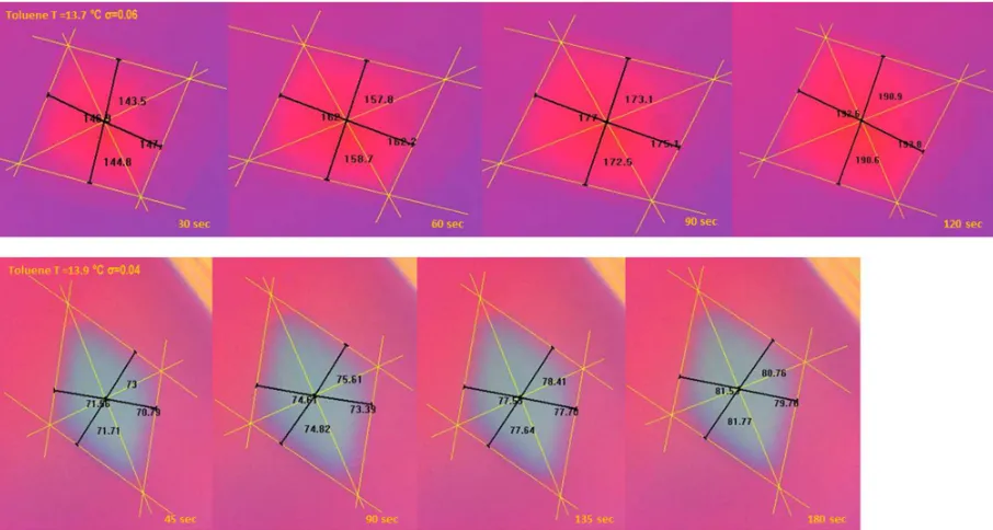
4. A sequence of images of methyl stearate crystals growing with time in three different

representative diesel type solvents.

(3)

[image:3.612.110.501.79.684.2]

1. Description of the methodology used to solve crystal morphology

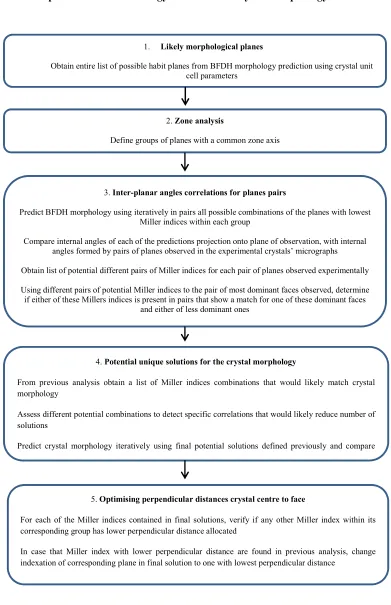
Fig. 1 Flow chart describing the procedure to follow for the morphology indexation of observed n-docosane crystals, using iterative predictions of the BFDH morphology “Reproduced from D.M. Camacho, K.J. Roberts, K. Lewtas, I. More. The crystal morphology and growth rates of triclinic n-docosane crystallising from n-dodecane solutions, Journal of Crystal Growth, 416 (2015) 47-56”.

4. Potential unique solutions for the crystal morphology

From previous analysis obtain a list of Miller indices combinations that would likely match crystal morphology

Assess different potential combinations to detect specific correlations that would likely reduce number of solutions

Predict crystal morphology iteratively using final potential solutions defined previously and compare 3. Inter-planar angles correlations for planes pairs

Predict BFDH morphology using iteratively in pairs all possible combinations of the planes with lowest Miller indices within each group

Compare internal angles of each of the predictions projection onto plane of observation, with internal angles formed by pairs of planes observed in the experimental crystals’ micrographs

Obtain list of potential different pairs of Miller indices for each pair of planes observed experimentally

Using different pairs of potential Miller indices to the pair of most dominant faces observed, determine if either of these Millers indices is present in pairs that show a match for one of these dominant faces

and either of less dominant ones 2. Zone analysis

Define groups of planes with a common zone axis

1. Likely morphological planes

Obtain entire list of possible habit planes from BFDH morphology prediction using crystal unit cell parameters

5. Optimising perpendicular distances crystal centre to face

For each of the Miller indices contained in final solutions, verify if any other Miller index within its corresponding group has lower perpendicular distance allocated

(4)

2. The complete set of planes delivered through the prediction of the BFDH morphology for methyl stearate crystals using three different sets of unit cell parameters

• Complete set of planes delivered by the prediction of the BFDH morphology for

orthorhombic methyl stearate crystals according to C.H. MacGillavry and M.

Wolthuis-Spuy, 1970. These planes are organised in nine different groups defined by

zone axis analysis.

Group 1/Zone axis [100]

hkl Mult dhkl Distance

{ 0 1 1} 4 7.33 13.64

{ 0 1 3} 4 7.16 13.96

{ 0 2 0} 2 3.68 27.20

{ 0 2 4} 4 3.63 27.52

{ 0 3 1} 4 2.45 40.81

{ 0 4 2} 4 1.84 54.43

{ 0 4 6} 4 1.83 54.76

{ 0 6 4} 4 1.22 81.70

Group 2/Zone axis [1-10]

{ 1 1 1} 8 4.46 22.44

{ 1 1 2} 8 4.44 22.51

{ 1 1 3} 8 4.42 22.63

{ 2 2 0} 4 2.23 44.82

{ 2 2 1} 8 2.23 44.84

{ 2 2 3} 8 2.23 44.94

{ 3 3 1} 8 1.49 67.24

{ 3 3 2} 8 1.49 67.27

(5)

{ 1 2 1} 8 3.07 32.53

{ 1 2 2} 8 3.07 32.58

{ 1 2 3} 8 3.06 32.66

{ 1 3 1} 8 2.25 44.53

{ 1 3 2} 8 2.24 44.56

{ 1 3 3} 8 2.24 44.63

{ 2 6 0} 4 1.12 89.03

{ 2 0 0} 2 2.81 35.63

{ 2 0 1} 4 2.81 35.65

{ 2 0 2} 4 2.80 35.69

{ 2 0 3} 4 2.80 35.77

{ 2 0 4} 4 2.79 35.88

{ 2 0 6} 4 2.76 36.19

{ 6 0 2} 4 0.94 106.92

{ 6 0 4} 4 0.93 106.98

{ 2 1 1} 8 2.62 38.15

{ 2 1 2} 8 2.62 38.20

{ 2 1 3} 8 2.61 38.27

{ 4 2 0} 4 1.31 76.28

{ 2 3 1} 8 1.85 54.17

{ 2 3 2} 8 1.84 54.21

{ 2 3 3} 8 1.84 54.26

{ 4 6 0} 4 0.92 108.33

(6)

{ 3 1 1} 8 1.81 55.16

{ 3 1 2} 8 1.81 55.19

{ 3 1 3} 8 1.81 55.24

{ 6 2 0} 4 0.91 110.30

{ 3 2 0} 4 1.67 59.97

{ 3 2 1} 8 1.67 59.98

{ 3 2 2} 8 1.67 60.01

{ 3 2 3} 8 1.67 60.05

monoclinic 2/ methyl stearate crystals according to S. Aleby, E. von Sydow, 1960. These

planes are organised innine different groups defined by zone axis analysis.

{ 0 1 1} 4 7.31 13.68

{ 0 1 3} 4 7.14 14.00

{ 0 2 0} 2 3.67 27.29

{ 0 2 4} 4 3.62 27.61

{ 0 3 1} 4 2.44 40.94

{ 0 4 2} 4 1.83 54.61

{ 0 4 6} 4 1.82 54.93

{ 0 6 4} 4 1.22 81.96

{ 1 1 1} 4 4.07 24.59

{ 1 1 3} 4 3.92 25.52

{ 1 1 -1} 4 4.20 23.81

{ 1 1 -3} 4 4.31 23.20

{ 2 2 0} 4 2.07 48.37

{ 2 2 4} 4 2.00 50.08

(7)

{ 3 3 1} 4 1.37 72.95

{ 3 3 -1} 4 1.39 72.16

{ 4 4 2} 4 1.03 97.53

{ 4 4 6} 4 1.01 99.25

{ 4 4 -2} 4 1.04 95.97

{ 4 4 -6} 4 1.06 94.57

{ 6 6 4} 4 0.68 146.71

{ 6 6 -4} 4 0.70 143.58

{ 1 2 0} 4 2.96 33.81

{ 1 2 2} 4 2.90 34.43

{ 1 2 -2} 4 3.00 33.31

{ 2 4 2} 4 1.47 68.21

{ 2 4 6} 4 1.44 69.56

{ 2 4 -2} 4 1.49 67.09

{ 2 4 -6} 4 1.51 66.22

{ 1 3 1} 4 2.19 45.76

{ 1 3 3} 4 2.16 46.26

{ 1 3 -1} 4 2.21 45.34

{ 1 3 -3} 4 2.22 45.02

{ 2 6 0} 4 1.10 91.08

{ 2 6 4} 4 1.09 92.00

{ 2 6 -4} 4 1.11 90.34

{ 2 0 0} 2 2.50 39.93

{ 2 0 2} 2 2.44 40.92

{ 2 0 4} 2 2.38 42.00

{ 2 0 6} 2 2.32 43.14

{ 2 0 -2} 2 2.56 39.03

{ 2 0 -4} 2 2.62 38.22

{ 2 0 -6} 2 2.67 37.52

{ 4 0 2} 2 1.24 80.84

(8)

{ 4 0 -2} 2 1.27 78.94

{ 4 0 -6} 2 1.29 77.23

{ 6 0 2} 2 0.83 120.76

{ 6 0 4} 2 0.82 121.75

{ 6 0 -2} 2 0.84 118.87

{ 6 0 -4} 2 0.85 117.97

{ 2 1 1} 4 2.34 42.66

{ 2 1 3} 4 2.29 43.64

{ 2 1 -1} 4 2.39 41.76

{ 2 1 -3} 4 2.44 40.96

{ 4 2 0} 4 1.18 84.40

{ 4 2 4} 4 1.16 86.28

{ 4 2 -4} 4 1.21 82.70

{ 2 3 1} 4 1.74 57.52

{ 2 3 3} 4 1.72 58.25

{ 2 3 -1} 4 1.76 56.86

{ 2 3 -3} 4 1.78 56.27

{ 4 6 0} 4 0.87 114.36

{ 4 6 4} 4 0.86 115.76

{ 4 6 -4} 4 0.88 113.11

{ 3 1 1} 4 1.62 61.90

{ 3 1 3} 4 1.59 62.88

{ 3 1 -1} 4 1.64 60.98

{ 3 1 -3} 4 1.66 60.12

{ 6 2 0} 4 0.81 122.87

{ 6 2 4} 4 0.80 124.77

{ 6 2 -4} 4 0.83 121.08

(9)

{ 3 2 0} 4 1.52 65.82

{ 3 2 2} 4 1.50 66.71

{ 3 2 -2} 4 1.54 64.99

{ 6 4 2} 4 0.75 132.52

{ 6 4 6} 4 0.74 134.35

{ 6 4 -2} 4 0.76 130.80

{ 6 4 -6} 4 0.77 129.19

monoclinic 2 methyl stearate crystals (I. More/Infineum UK, personal communication,

July 25, 2014). These planes are organised in nine different groups defined by zone axis

analysis.

{ 0 2 0} 1 3.70 27.03

{ 0 2 1} 2 3.69 27.13

{ 0 2 2} 2 3.65 27.43

{ 0 2 3} 2 3.58 27.92

{ 0 2 4} 2 3.50 28.60

{ 0 2 6} 2 3.28 30.44

{ 0 6 2} 2 1.23 81.22

{ 0 6 4} 2 1.23 81.62

Group 2/Zone axis [-100]

{ 0 -2 0} 1 3.70 27.03

{ 0 -2 1} 2 3.69 27.13

{ 0 -2 2} 2 3.65 27.43

{ 0 -2 3} 2 3.58 27.92

{ 0 -2 4} 2 3.50 28.60

{ 0 -2 6} 2 3.28 30.44

{ 0 -6 2} 2 1.23 81.22

{ 0 -6 4} 2 1.23 81.62

(10)

{ 1 1 -3} 2 4.45 22.48

{ 1 1 -2} 2 4.39 22.80

{ 1 1 -1} 2 4.28 23.36

{ 1 1 0} 2 4.14 24.13

{ 1 1 1} 2 3.98 25.10

{ 1 1 2} 2 3.81 26.24

{ 1 1 3} 2 3.63 27.53

{ 2 2 -3} 2 2.17 46.11

{ 2 2 -1} 2 2.11 47.44

{ 2 2 1} 2 2.03 49.18

{ 2 2 3} 2 1.95 51.29

{ 3 3 -2} 2 1.41 70.78

{ 3 3 -1} 2 1.40 71.56

{ 3 3 1} 2 1.36 73.30

{ 3 3 2} 2 1.35 74.27

Group 4/Zone axis [-1-10]

{ 1 -1 -3} 2 4.45 22.48

{ 1 -1 -2} 2 4.39 22.80

{ 1 -1 -1} 2 4.28 23.36

{ 1 -1 0} 2 4.14 24.13

{ 1 -1 1} 2 3.98 25.10

{ 1 -1 2} 2 3.81 26.24

{ 1 -1 3} 2 3.63 27.53

{ 2 -2 -3} 2 2.17 46.11

{ 2 -2 -1} 2 2.11 47.44

{ 2 -2 1} 2 2.03 49.18

{ 2 -2 3} 2 1.95 51.29

{ 3 -3 -2} 2 1.41 70.78

{ 3 -3 -1} 2 1.40 71.56

{ 3 -3 1} 2 1.36 73.30

{ 3 -3 2} 2 1.35 74.27

{ 1 3 -3} 2 2.26 44.34

{ 1 3 -2} 2 2.25 44.51

{ 1 3 -1} 2 2.23 44.80

(11)

{ 1 3 1} 2 2.19 45.73

{ 1 3 2} 2 2.16 46.36

{ 1 3 3} 2 2.12 47.10

{ 1 -3 -3} 2 2.26 44.34

{ 1 -3 -2} 2 2.25 44.51

{ 1 -3 -1} 2 2.23 44.80

{ 1 -3 0} 2 2.21 45.20

{ 1 -3 1} 2 2.19 45.73

{ 1 -3 2} 2 2.16 46.36

{ 1 -3 3} 2 2.12 47.10

{ 2 0 -6} 2 2.78 35.92

{ 2 0 -4} 2 2.72 36.74

{ 2 0 -3} 2 2.68 37.36

{ 2 0 -2} 2 2.62 38.11

{ 2 0 -1} 2 2.56 38.99

{ 2 0 0} 2 2.50 39.99

{ 2 0 1} 2 2.43 41.09

{ 2 0 2} 2 2.36 42.30

{ 2 0 3} 2 2.29 43.59

{ 2 0 4} 2 2.22 44.98

{ 2 0 6} 2 2.09 47.96

{ 6 0 -4} 2 0.86 116.05

{ 6 0 -2} 2 0.85 117.93

{ 6 0 2} 2 0.82 122.14

{ 6 0 4} 2 0.80 124.45

{ 2 4 -6} 2 1.54 64.90

{ 2 4 -4} 2 1.53 65.36

{ 2 4 -2} 2 1.51 66.14

{ 2 4 0} 2 1.49 67.24

{ 2 4 2} 2 1.46 68.64

(12)

{ 2 4 6} 2 1.38 72.26

{ 2 -4 -6} 2 1.54 64.90

{ 2 -4 -4} 2 1.53 65.36

{ 2 -4 -2} 2 1.51 66.14

{ 2 -4 0} 2 1.49 67.24

{ 2 -4 2} 2 1.46 68.64

{ 2 -4 4} 2 1.42 70.32

{ 2 -4 6} 2 1.38 72.26

{ 3 1 -3} 2 1.70 58.74

{ 3 1 -2} 2 1.68 59.58

{ 3 1 -1} 2 1.65 60.49

{ 3 1 0} 2 1.63 61.48

{ 3 1 1} 2 1.60 62.55

{ 3 1 2} 2 1.57 63.68

{ 3 1 3} 2 1.54 64.87

{ 3 -1 -3} 2 1.70 58.74

{ 3 -1 -2} 2 1.68 59.58

{ 3 -1 -1} 2 1.65 60.49

{ 3 -1 0} 2 1.63 61.48

{ 3 -1 1} 2 1.60 62.55

{ 3 -1 2} 2 1.57 63.68

{ 3 -1 3} 2 1.54 64.87

{ 4 2 -6} 2 1.26 79.45

{ 4 2 -4} 2 1.24 80.87

{ 4 2 -2} 2 1.21 82.53

(13)

{ 4 2 2} 2 1.16 86.51

{ 4 2 4} 2 1.13 88.81

{ 4 2 6} 2 1.10 91.28

{ 4 -2 -6} 2 1.26 79.45

{ 4 -2 -4} 2 1.24 80.87

{ 4 -2 -2} 2 1.21 82.53

{ 4 -2 0} 2 1.18 84.42

{ 4 -2 2} 2 1.16 86.51

{ 4 -2 4} 2 1.13 88.81

{ 4 -2 6} 2 1.10 91.28

{ 4 6 -6} 2 0.91 110.26

{ 4 6 -4} 2 0.90 111.28

{ 4 6 -2} 2 0.89 112.50

{ 4 6 0} 2 0.88 113.89

{ 4 6 2} 2 0.87 115.45

{ 4 6 4} 2 0.85 117.18

{ 4 6 6} 2 0.84 119.06

{ 4 -6 -6} 2 0.91 110.26

{ 4 -6 -4} 2 0.90 111.28

{ 4 -6 -2} 2 0.89 112.50

{ 4 -6 0} 2 0.88 113.89

{ 4 -6 2} 2 0.87 115.45

{ 4 -6 4} 2 0.85 117.18

{ 4 -6 6} 2 0.84 119.06

{ 6 4 -6} 2 0.79 126.47

{ 6 4 -4} 2 0.78 128.02

(14)

{ 6 4 0} 2 0.76 131.58

{ 6 4 2} 2 0.75 133.56

{ 6 4 4} 2 0.74 135.68

{ 6 4 6} 2 0.73 137.93

{ 6 -4 -6} 2 0.79 126.47

{ 6 -4 -4} 2 0.78 128.02

{ 6 -4 -2} 2 0.77 129.73

{ 6 -4 0} 2 0.76 131.58

{ 6 -4 2} 2 0.75 133.56

{ 6 -4 4} 2 0.74 135.68

(15)

3. Derivation of models expressions for the assessment of the dependence of single faces growth rates on supersaturation

Growth models have been developed which depend upon the nanostructure of the crystal

surfaces describing three distinct mechanism of crystal growth.

If a crystal face is molecularly rough, there are many kinks sites on the surface through which

the growth of the face will proceed. The growth / is then said to be continuous (or

normal) and can be described by the Rough Interface Growth (RIG) model [21]

given by

equation (1)

= (1)

where is the growth rate constant and the solution´s relative supersaturation at the

interface

A second possibility is that the crystal face is molecularly smooth and therefore growth is

then nucleation mediated. For faces molecularly smooth growth can proceed only after the

face roughens by nucleation of 2 clusters, with edges having enough growth sites on them.

The spreading of the 2 clusters is what fills a crystal monolayer and this leads to the growth

of the crystal face. This mechanism is described by the Birth and Spread (B&S) model given

by equation (2)

= /exp

(16)

where is given by

= −!"#$ #

3&# (3)

In this expression "_#$is the interfacial tension of the 2 nucleus

And finally, in the presence of points of emergence of screw dislocations, the crystal face is

stepped and exhibits spirals (or screw dislocations). In this case the growth rate is limited by

the integration of a growth unit into the crystal, at a step generated by lattice defects on the

surface and the dependence of the growth rate on supersaturation can be described by the

Burton-Cabrera-Frank (BCF) model [20] given by equation (4)

= #'ℎ #

(4)

For all of the three models ∝ * where * is a kinetic coefficient that characterises the rate

with which the growth units are incorporated into the lattice at the step. This rate is limited

first of all, by de-solvation of the kinks and of the incorporating species and secondly, by the

formation of new kinks at the surface of the crystal.

A general formula for the face of a crystal growing with time is given by

(17)

This law clearly described the RIG model and also represents the two limiting cases of the

BCF equation , = 1 or 2. It can make a satisfactory approximation of the B&S model in a

limited range of high supersaturation [19].

Given the experimental method used to collect crystals´ growth rates, the measured growth

rates are not only influenced by the incorporation of growth units into the crystal surface, but

also by the diffusion of the growth units within the bulk of the solution. Thus, this effect

needs to be accounted for. In this case volume diffusion is followed by a “docking rate” that

includes the effect of any of the three mechanisms on the crystal surface described by

equations (1) to (4). As these two effects act consecutively, they have to share the driving

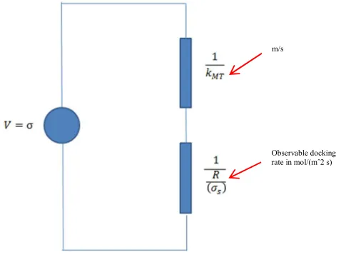
force and the slower one will be rate determining [18]. Making an analogy to a circuit in which the resistors are arranged in a chain, the process can be represented by Fig. 2. This shows that

the resistance to the diffusion of growth units in the bulk of the solution is given by the

inverse of the mass transfer coefficient ₀₁ and the resistance to mass transfer on the surface

[image:17.612.223.462.458.638.2]

of the crystal is given by the inverse of the “observable docking rate”.

Fig. 2 Representation of the mass transfer process for the growth of crystal ´s single faces by an analogy to a circuit in which resistors are in series according to V=IR. V represents the driving force, I the flow of molecules towards the surface and R the resistant to this flow

(18)

If mass transfer on the surface is taken as a first order process then the rate of transfer ,₀₁ is

given by

,01= 2− 3 (6)

where ₂ is the observed incorporation rate constant, the concentration at the crystal

solution interface and ₃ is the concentration at equilibrium

Given that ,₀₁ is related to the rate of growth of a single face by

,01= 3 (7)

Then

2=

(8)

where = 45₅6 7− 18

Similarly mass transfer 9& would be represented by

9&

= 01 − = 2− 3 (9)

(19)

9&

= 01 − = − 3 (10)

where ₀₁ is the coefficient of mass transfer within the bulk of the solution, the solution

concentration and is the effective mass transfer area

Expressing all terms in equation (10) using absolute supersaturation it becomes

9&

= 01 − 3 =

:

9;33 (11)

where : is the solute density and 9; the solute molecular weight

Rearranging

− = 9&

013 (12)

and

= 9&

:

9;

(13)

Thus summing driving forces

9&

= 1 1

013+

1

:

9;

(20)

Multiplying the denominator by _=>6 ?6

and making ₀₁´ 4A

8 =

B=C57 0D6

E6 the growth of a

crystal face with time can be expressed as

4_{8 =} ₁ 1

01´ + 1

(15)

Specific models describing the kinetics on the crystal surface can be inserted into equation

(15) as would depend on the mechanism with which the growth units will be attached to the

crystal face. Thus using the power law given by equation (5) and additionally assuming

≈

4_{8 =} ₁ 1

01´ +

1

+G

₍₁₆₎

Similarly for B&S crystal growth mechanism using equation (2)

4_{8 =} ₁ 1

01´ +

1

G/exp 4 ₈

(17)

And for the BCF crystal growth mechanism using equation (4)

4_{8 =} ₁ 1

01´ +

1

'ℎ 4 ₈#

(21)

(22)

[image:22.612.104.557.46.288.2]