White Rose Research Online URL for this paper:
http://eprints.whiterose.ac.uk/132893/
Version: Accepted Version
Proceedings Paper:
Escolano, Francisco and Hancock, Edwin R orcid.org/0000-0003-4496-2028 (2018) Bragg
Diffraction Patterns as Graph Characteristics. In: Eleventh International Conference on
Energy Minimisation Methods in Computer Vision and Pattern Recognition. Lecture Notes
in Computer Science . Springer Nature , pp. 59-72.
https://doi.org/10.1007/978-3-319-78199-0_5
[email protected] https://eprints.whiterose.ac.uk/
Reuse
Items deposited in White Rose Research Online are protected by copyright, with all rights reserved unless indicated otherwise. They may be downloaded and/or printed for private study, or other acts as permitted by national copyright laws. The publisher or other rights holders may allow further reproduction and re-use of the full text version. This is indicated by the licence information on the White Rose Research Online record for the item.
Takedown
If you consider content in White Rose Research Online to be in breach of UK law, please notify us by
Characteristics
Francisco Escolano and Edwin R. Hancock
Department of Computer Science and AI, University of Alicante, 03690, Alicante Spain
Department of Computer Science, University of York, York, YO10 5GH, UK
Abstract. In this paper we establish a link between diffraction theory
and graph characterization through the Schr¨odinger operator. This pro-vides a natural way of characterizing wave propagation on a graph. In order to do so, we compute the spatio-temporal Fourier transform of the operator and then pack its spherical representation in a point of a Stiefel manifold. We show that when the temporal interval of analysis is set according to quantum efficiency principles the proposed approach outperforms the alternatives in graph discrimination.
Keywords: Diffraction, Schr¨odinger operator, Stiefel manifolds.
1
Introduction
Graph characterization aims to provide a succinct way of representing graph structure that can be used distinguish or compare different types of graph, with-out applying graph or subgraph isomorphism (procedures that are known to be NP-complete). Popular and effective methods include random walks [1], the Ihara zeta function [2] and the spectral radius [3].
equation. It provides a method to represent the heat transfer between the nodes of a graph over time.
Closely related to this work on the heat kernel is the wave kernel signature (WKS) [7]. This involves histogramming the elements of the wave kernel, which is the solution of the complex wave equation or Schr¨odinger equation associated with the graph’s Laplacian matrix. While the heat equation describes how heat is transferred in a system, the Schr¨odinger equation characterizes the dynamics of a particle in a quantum system. In fact, the continuous time quantum walk on a graph is the solution to the Schr¨odinger equation, with the normalised Laplacian playing the role of a Hamiltonian. In this setting, the quantum nature of the Schr¨odinger equation and its complex-valued solutions give rise to many interesting non-classical effects, including quantum interferences. These interfer-ences have proved to be useful in several applications, including the detection of symmetric motifs in graphs via continuous-time quantum walks [8] and graph embedding by means of quantum commute times [9].
One difference between the approach in [7] and ours is that in the WKS, the time variable is not considered. In order to do so, the limiting average time behaviour (in the infinity) is computed. However, Rossi et al. [8] show that this choice is sub-optimal when used for measuring the similarity between two graphs. Alternatively, our approach relies on choosing proper finite limiting times. Our process is data driven (validated by the experiments) but herein we argue in favor of relating these limiting times with thetransport efficiencyof the quantum walk. Therefore, the long-term objective of this line of research is to choose the limiting times thatmaximize transport efficiency.
Another difference between WKS and our representation is that we do not compare the wave signatures between two nodes in the graph, but consider si-multaneously all of them as forming a time-parameterized wave.
It must be stressed though that we do not claim that our method is in any sense a quantum algorithm. So we do not consider the issue of whether the char-acterization developed is observable or not. We are primarily interested in the complex nature of the characterization provided by the Schr¨odinger equation and the resulting non-stationarity and non-ergodicity of the dynamic system as-sociated with it. Since the dynamic system is non-stationary and non-ergodic, it makes sense neither to characterize it using its steady state behaviour (since this does exist) nor its phase transitions (as is the case in the heat flow method). In-stead we turn to the Fourier transform as a natural way of providing a frequency domain characterization of the time evolution of the complex wave equation, and use this instead of the heat flow trace [4].
sym-metry planes of the graph-structure are manifest as sets of geometrically regular frequency peaks. Thus we transform the characterzation of graph structure into a problem of searching for geometric regularity in a set of points.
In Section 2 we compare the Schr¨odinger operator with the heat kernel (both are governed by the eigensystem of the graph Laplacian). In Section 3 we analyze the operator and build a parametric representation from its spatio-temporal power spectrum. Such representation is transferred to a point in a suitable Stiefel manifold and principal angles are used for graph comparison. In Section 4 we show that the proposed approach outperforms state-of-the-art graph matching methods. Finally, in Section 5 we present our conclusions and future work.
2
Heat Kernel Vs. Schr¨
odinger Operator
2.1 Heat Kernel
LetG= (V, E) be an undirected graph whereV is its set of nodes andE⊆V×V
is its set of edges. The Laplacian matrixL=D−Ais constructed from then×n
adjacency matrixAwithn=|V|, in which the elementA(u, v) = 1 if (u, v)∈E
and 0 otherwise, where the elements of the diagonal n×n degree matrix are
D(u, u) = P
v∈V A(u, v). The n×n heat kernel matrix Kt is the fundamental
solution of the heat equation
∂Kt
∂t =−LKt, (1)
and depends on the Laplacian matrixLand timet. The form of the heat kernel matrix is Kt = e−Lt. The continuous time random walk starting at p0 ∈ Rn evolves as pt =Ktp0, wherept is the state of the random walk at timet. The
spectral decomposition of the Laplacian isL=ΦΛΦT, whereΦ= [φ
1|φ2|. . .|φn]
is the n ×n matrix of ordered eigenvectors according to the corresponding eigenvalues 0 = λ1 ≤ λ2 ≤ . . . ≤ λn, and Λ = diag(λ1λ2 . . . λn).
There-fore, the spectral decomposition of the heat kernel is Kt = Φe−ΛtΦT where
e−Λt =diag(e−λ1te−λ2t . . . e−λnt), that is, the heat kernel and the Laplacian share their eigenfunctions, which are contained inΦ. Both the columns and the rows ofΦdefine orthonormal basis:φT
i φj=δij.
2.2 Schr¨odinger Operator
The Schr¨odinger equation describes how the complex state vector|ψti ∈Cn of
a continuous-time quantum walk varies with time [10]:
∂|ψti
∂t =−iL|ψti. (2)
Given an initial state|ψ0i the latter equation can be solved to give|ψti=
Ψt|ψ0i, whereΨt=e−iLtis a complexn×nunitary matrix. In this paper we refer
itself and not on the quantum walk process. In this regard, Stone’s theorem [13] establishes a one-to-one correspondence between a time parameterized unitary matrix Ut and a self-adjoint (Hermitian) operator H = H∗ such that there is
a unique Hermitian operator satisfying U = eitH. Such an operator H is the
Hamiltonian. In the case of graphs we may set H =−Land then we have that
Ψt=e−itLis a unitary matrix fort∈R.
Unitary matrices play a fundamental role in characterizing complex wave equationsin a manner analogous to that performed by doubly stochastic matrices in characterizing diffusion processes. A n×n complex matrix U is unitary if
U†U =U U† = I
n, where U† is the conjugate transpose, that is (A†)ij =Aji.
Therefore, both the rows and columns ofU form a orthonormal basis in Cn.U
is diagonalizable via the factorizationU =V ΛV† whereΛcontains the complex
eigenvalues of U and V is unitary and its columns contain the eigenvectors of
U. Combining the latter diagonalization with the property|det(U)|= 1 we have that all the complex eigenvalues of U must lie on the unit Argand circle. They must have either the formeiθ ore−iθ whereθis a rotation angle. More precisely,
for Ψt we obtain the spectral decompositionΨt =Φe−itΛΦT, where Φcontains
the eigenvectors of L and e−iΛt = diag(e−iλ1te−iλ2t . . . e−iλnt), the complex eigenvalues ofΨt, rely on the ones of the Laplacian.
Therefore, the Laplacian controls the dynamics of both the heat kernel and the Schr¨odinger operator according to the similarity between Eq. 2 and Eq. 1. However, this similarity is misleading since Ψt is complex valued. The physical
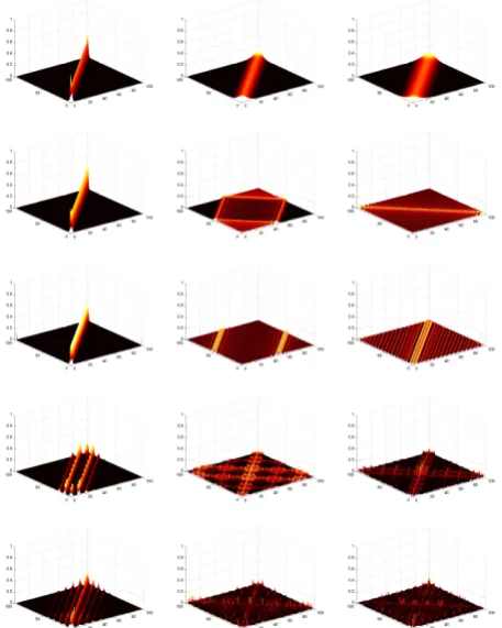
dynamics induced by the Schr¨odinger equation is therefore totally different from that of the heat equation, due to the existence of oscillations and interferences. In this paper we address the question of whether the Schr¨odinger operator may be used to characterize the structure of a graph. Empirical analysis on dif-ferent graph structures shows that both the heat kernel and the Schr¨odinger operator evolve with time in a manner which strongly depends on graph struc-ture. 1 However, the underlying physics and the resulting dynamics are quite different (see Fig. 1 where for the heat kernel we representKt(u, v) and for the
Schr¨odinger operator we show the squared magnitude |Ψt(u, v)|2). In the case
of heat flow, heat diffuses between nodes through the edges, eventually creating transitive links (allowing effective energy exchange between nodes that are not directly connected by an edge), until reaching a stationary equilibrium state. The Schr¨odinger operator defines a wave which yields a faster energy propaga-tion through the system (e.g. for a 100 nodes line graph, it takes t = 50 time steps for the Schr¨odinger operator to reach every possible position on the graph, taking more than twice this time in the case of the heat kernel [4]). Moreover, due to the negative components of the complex amplitudes, interferences are created, producing energy waves [5]. The main difference is that because of its wave nature the Schr¨odinger operator never reaches an equilibrium state. In other words, it is non-ergodic. Graph connectivity imposes constraints on the distribution of energy. In the case of the heat kernel, a larger number of
en-1 Videos showing the evolution of both heat kernel and Schr¨odinger operator are
ergy distribution constraints implies the creation of more transitive links with time [4]. This is true in the case of the Schr¨odinger operator, for which higher frequency and more symmetrical energy distribution patterns are also observed.
Fig. 1.Evolution with time (t= 1,25 and 100). From top to bottom: heat kernel for
a 100 node line graph, Schr¨odinger operator for a 100 node line graph, Schr¨odinger operator for a 100 node circle graph, Schr¨odinger operator for a 10×10 grid graph
with 4 neighbour connectivity and Schr¨odinger operator for a 10×10 grid graph with
8 neighbour connectivity. (Courtesy of Pablo Suau)
3
Analysis of the Schr¨
odinger Operator
3.1 Non-Ergodicity
Φe−tΛΦT, that is
Ψt= n
X
k=1
e−itλkφ
kφTk andKt=
n
X
k=1
e−tλkφ
kφTk, (3)
where λk is the k-th eigenvalue of the Laplacian L and φk its corresponding
eigenvector. Therefore, both operators are specified by the eigenfunctions of the Laplacian but in a very different way. The spectral decomposition of the heat kernel demonstrates that it is dominated by the lowest eigenvalues, due to the fact that limt→∞e−tλk = 0. However, the limit ofe−itλk = cos(tλk)−isin(tλk)
whent tends to infinity is undefined. Thus, there are two important differences with the heat kernel. Firstly, the Schr¨odinger operator never converges (it is non-ergodic), and secondly, it is not dominated by any particular eigenvalue. This is consistent with the well known physics of waves since the Schr¨odinger operator is a linear combination of waves.
3.2 Regimes Dynamics of Wave Propagation
The behavior of the Schr¨odinger operator at small and large times responds to different aspects of graph structure. At lowt, the edge constraints contained in the Laplacian dominate (see left column in Fig. 1). At hight, on the other hand, it is the path structure that dominates (see the rest of the columns in Fig. 1).
In addition, the two regimes can be explained by the fact that the largest am-plitudes occur at low frequencies. More precisely, each entryΨt(u, v) is described
by alinear combination of complex rotations:
Ψt(u, v) =
Pn
k=1e−iλktφk(u)φk(v) ifu6=v
Pn
k=1e−iλktφ2k(u) otherwise.
(4)
We let zk(u, v) = φk(u)φk(v) if u 6= v and zk(u, v) = φk(u)2 otherwise. In
this case zk(u, v) ∈ R for each value relies on the k−th eigenvector φk of the
Laplacian. Since
|Ψt(u, v)|2= n
X
k=1
n
X
l=k
zk(u, v)zl(u, v)2 cos(t(λl−λk)) (5)
we have that
lim
t→0|Ψt(u, v)| 2= 2
n
X
k=1
n
X
l=k
zk(u, v)zl(u, v) (6)
yields the maximal amplitude at (u, v) since zk(u, v) andzl(u, v) are time
inde-pendent. Astincreases the differencesλl−λk, which are also time independent,
become significant. They define lower or equal amplitudes and the characteristic frequency content of the wave emerges as expected. Low amplitudes dominate due to the ordering of the eigenvectors of the Laplacian 0 =λ1≤λ2≤. . .≤λn
although there are always n terms whereλl =λk. The latter property
0 50 100 150 200 250 300 350 400 0 2 4 6 8 10
12 LAPLACIAN EIGENVALUES CIRCLE GRID 4N GRID 8N LINE
0 1 2 3 4 0 500 1000 1500 2000 2500 CIRCLE
0 1 2 3 4 0 500 1000 1500 2000 2500 LINE
0 2 4 6 8 0 500 1000 1500 2000 2500 GRID 4N
[image:8.595.175.440.119.256.2]0 2 4 6 8 1012 0 500 1000 1500 2000 2500 3000 GRID 8N
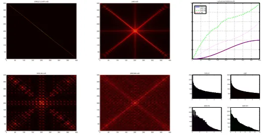
Fig. 2.Power spectra of the Schr¨odinger operator for different graphs of 400 nodes at
t= 25: circle (loop) graph (top-left), line graph (top-middle), 20×20 grid graph with 4
neighbor connectivity (bottom-left) and 20×20 grid graph with 8 neighbor connectivity.
For the latter graphs we also show their spectra (top-right) and the multiplicity of each value of∆kl(bottom-right).
3.3 Expressiveness of the Schr¨odinger Power Spectra
The discrete Fourier transform (DFT) of the squared magnitude of the Schr¨odinger Operator Ψtis
Ft(ωu, ωv) = n
X
u,v=1
|Ψt(u, v)|2e−i(ωuu+ωvv)
= n X u,v=1 n X
k=1,l=k
Zklδ(t∆kl−(ωuu+ωvv))+
n
X
k=1,l=k
Zklδ(t∆kl+ (ωuu+ωvv))
, (7)
where ωu and ωv are the angular frequencies, ∆kl = λl−λk ≥ 0, Zkl =
zk(u, v)zl(u, v), and δ(.) is the Dirac delta function resulting from the Fourier
transforms of 2 cos(t(∆kl)) = eit∆kl +e−it∆kl (see Eq. 5) for k = 1, . . . , n,
l=k, . . . , n. After shifting we have that the amplitudeAt(ωu, ωv) =|Ft(ωu, ωv)|
is given by pooling the values relying on Pn
k=1,l=kZkl at all points (u, v)
be-longing to the linest∆kl =ωuu+ωvv(t∆kl gives the distance to the origin and
the vector [ωu, ωv]T is perpendicular to the direction of the line). Therefore the
energy (power) distribution is determined by both the spectrum of the Lapla-cian, which defines the gaps∆kl, and its eigenvectors which define the values of
Pn
k=1,l=kZkl.
diffraction gratings (interference patterns). In diffraction theory, interference patterns emerge when waves are bent around edges or slits. Constructive and destructive interferences occur producing alternate bright and dark fringes (see for instance the Young’s experiment) which fade away from the center. The distribution of the so called Bragg’s peaks (associated to constructive interfer-ences) relies both on wavelengths and the number and spacings between the slits, as well as it also depends on the incidence angle. Fringes become sharper, for instance, as the number of slits is increased but, in this case, they are char-acterized by less and less significant maxima of intensity. In X-ray crystallogra-phy, the interdependence between the spatial distribution (e.g. a lattice) of the atoms, the properties of incident light and diffraction patterns is exploited to infer the tridimensional density of electrons in a crystal as well as to solve the structure of organic molecules like proteins. When applying this ideas to charac-terize pure topological structures like graphs, we realized that the Schr¨odinger operator provides a natural way of encoding the latter interdependences: the complex exponentiation of the Hamiltonian (the negative Laplacian) produces a wave equation completely determined by the spectrum and eigenvectors of such Hamiltonian. In addition, there is a correspondence between interference pat-terns and Fourier transforms. Actually, the Fourier transform in Eq. 7 has the same form of an aperture used in Fraunhofer diffraction:a[δ(x−S/2)+δ(x+S/2)] where S is the distance between two slits. This gives us an interpretation of
A[δ(t∆kl−(ωuu+ωvv))+δ(t∆kl+(ωuu+ωvv))] whereA=Pnu,v=1
Pn
k=1,l=kZkl
in terms of the topological constraints that must be satisfied in order to produce Bragg’s peaks. In our case, the role of the slits is played by the spectra (more precisely by the gaps∆kl) and the eigenvectors of the Laplacian. They determine
what frequencies (energies in the power spectra) can be seen in the diffraction pattern. For instance, in circle (ring) graphs Fig. 2 (top-left) shows that the energy distribution may be constrained to lie at 0 = u+v. For a line (path) graph (top-middle) we have a richer energy distribution although the line and circle graphs are quasi iso-spectral. Grid graphs are endowed with even richer diffraction patterns (larger range of eigenvalues).
20 40 60 80 50 100 150
20 40 60 80 50 100 150
20 40 60 80 50 100 150
20 40 60 80 50 100 150
20 40 60 80 50 100 150
20 40 60 80 50 100 150
20 40 60 80 50 100 150 0 0.02 0.04 −0.04 −0.02 0 0.02 −0.04 −0.02 0 0.02 0.04 −0.04 −0.02 0 0.02 0.04 −0.05 0 0.05 −0.05 0 0.05 −0.06 −0.04 −0.02 0 0.02 0.04
20 40 60 80 50 100 150 −0.2 −0.1 0
20 40 60 80 50 100 150 −0.1 −0.05 0 0.05
[image:10.595.186.430.108.293.2]20 40 60 80 50 100 150 −0.05 0 0.05
Fig. 3.Spatio-Temporal Power spectra of the Schr¨odinger operator for a 20×20 grid
graph with 4 neighbor connectivity. Top-left: planes ωu = 0, ωv = 0, ωt′ = 0. Top-center/right: detail ofωt′= 0 andωt′= 3 showing parallel high pooled lines. Bottom-left: spherical coordinates of log-amplitudes. Bottom-right: 10 principal eigenvectors of theθ−φspace.
3.4 Characterization of the Spatio-Temporal Schr¨odinger Power Spectra
Let F(ωu, ωv, ωt) be the spatio-temporal DFT of|Ψ(u, v, t)|2. It is
straightfor-ward to extend Eq. 7 to include time variation. As expected, after shifting the transform we have that the amplitudesA(ωu, ωv, ωt) =|f(ωu, ωv, ωt)|are given
by pooling the values relying on Pn
k=1,l=kZkl at all points (u, v, t) belonging
to the planes t∆kl = ωuu+ωvv+ωtt. Furthermore, since the gaps ∆kl are
time independent, scaled temporal frequenciesωttcan be seen as offsets in the
spatial constraints t∆kl = ωuu+ωvv. Such offsets are needed to explain the
spatio-temporal behavior of the Schr¨odinger operator. More precisely, fort >0 and ωt6= 0 only the contributions Pnk=1,l=kZkl at (u, v, t) where (u, v) do not
satisfyt∆kl =ωuu+ωvv are taken into account for computing the amplitudes
A(ωu, ωv, ωt).
An interesting particular case of the latter rationale is to pool amplitudes from (u, v) satisfying constraints which are orthogonal to the spatial ones. For instance, in Fig. 3 (top-left) we show the spatio-temporal log-amplitudes for the planeswu= 0,wv= 0 andwt′ = 0 wheret′=t−T /2 being [0, T] the temporal interval of analysis. The graph analyzed is the 20×20 grid with 4 neighbors con-nectivity. In Fig. 3 (top-center/right) we show respectively the planes ωt′ = 0 and ωt′ = 3. Both of them are characterized by high log-amplitudes at lines
wv = wu±k, with k ≥ 0, which are orthogonal to those which have a
simi-lar degree of pooling at a particusimi-lar t′ (see Fig. 2 (bottom-left)). The highest
in-100 101
102 103
104 10−7
10−6 10−5 10−4 10−3 10−2 10−1 100
t
Energy
QUANTUM EFFICIENCY FOR GATOR#1
Probability Envelope
100
101
102
103
104
10−8
10−6
10−4
10−2
100
t
Energy
QUANTUM EFFICIENCY FOR GATOR#20 Probability Envelope
0 10 20 30 40 50 60 70 80 90 100 0
0.1 0.2 0.3 0.4 0.5 0.6 0.7 0.8 0.9
PERFORMANCE FOR GATORBAIT
Retrieval (X axis) vs Average Recall (Y axis) Bragg <T>=100
Bragg <T>=64 Bragg T=10 Bragg T=4
0 10 20 30 40 50 60 70 80 90 100 0
0.1 0.2 0.3 0.4 0.5 0.6 0.7 0.8 0.9
Retrieval (X axis) vs Average Recall (Y axis) PERFORMANCE FOR GATORBAIT
[image:11.595.151.462.194.507.2]Entropic Alignment Bragg Characteristics PATH Algorithm Caelli−Kosinov
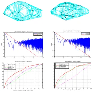
Fig. 4.Experimental Results. Top: Delaunay graphs of Gatorbait - Gator#1 (left)
creases. This happens for sign(ωu) =sign(ωv). Otherwise we have the inverse
case: log-amplitudes increase with|k|(atωt′ = 0 such increase is more spatially constrained than atωt′ = 3).
Once the role of temporal frequencies is clarified, it is convenient to change the coordinate system in order to better visualize the angular asymmetries in the spatio-temporal domain (anisotropy). Given (ωu, ωv, ωt) its spherical coordinates
are given by (r, θ, φ) where r =p
ω2
u+ω2v+ω2t is the radius, θ = tan−1(ω
v
ωu), −π ≤θ ≤π is the azimuthal angle in the ωu−ωv plane and φ= cos−1(ωrt),
−π2 ≤φ≤ π2 is the elevation angle. Therefore, rencodes the magnitude of the spatio-temporal frequencies, θrefers to the relation between spatial frequencies and φgives the relative importance of temporal frequencies. In addition, for a given pairαs= (θ, φ) the power spectrumA(αs)2decays withrand such decay
does not follows, in general, a power law. In addition, forαs+∆= (θ+∆, φ+∆),
with |∆| >0 as small as possible, we have that A(αs+∆)2 differs significantly
fromA(αs)2 in the general case (directional anisotropy).
In Fig. 3 (bottom-left) we plot the r−θ−φ space for the log-amplitudes. The representation is symmetric with respect to the elevation axis θ = 0 and it is periodic with respect to the azimuthal axisφ= 0. Therefore, for the sake of computational efficiency we can define a discrete θ−φ elevation-azimuth space by setting:θ∈[0, π/2],φ∈[0, π]. Such space relates spatial and temporal frequencies. In addition, for each discrete radiusr∈[0, rmax], wherermax=n/2,
we define asample spaceXras the log-amplitudes logA(r, αs) at all coordinates
of the θ−φ parametric space. Performing SVD/PCA analysis on the set of sample spaces S = {Xr} the principal eigenvalues λ1 ≥ λ2 ≥ . . . ≥ λp with
p≪d, whered=δθ×δφ is the number of cells, encode the degree of directional
anisotropy. Their associated d−dimensional eigenvectors u1, u2, . . . , up define a
subspace where we compress all the spatio-temporal information of the operator. The latter representation allows us to map a graph to a multi-layered para-metric space (one layer per radial samples). Then, such space is encoded by a set of eigenvectors as it is done when analyzing image sequences. In this regard, it becomes very useful to consider each set of eigenvectors (subspace) as a point in a given manifold in order to exploit the geodesics defined in it. The natural choice is to consider that U = [u1u2 . . . up] is a point in the Stiefel manifold
St(p, d) = {U ∈ Rd×p : UTU = I
p}, that is, the set of d×p matrices with
orthonormal columns [16]. In Fig. 3 (bottom-right) we show the first p = 10 eigenvectors which define the Stiefel point associated to the 20×20 4N grid graph. Given the spatial structure of log-amplitudes in spherical coordinates, global details appear close toπ/2 in the azimuthal axis whereas local details are highlighted at lower values.
andSpan(V) satisfy that cos(θi) are the singular values ofUTV and the geodesic
distance betweenUandV is given by||Θ||whereΘ= [θ1θ2. . . θp]. In this paper,
given two graphs GX = (VX, EX) and GY = (VY, EV) and the Stiefel points
UX andUY derived from the corresponding spatio-temporal Schr¨odinger power
spectra, we will quantify the dissimilarity between the two graphs in terms of the principal angles.
4
Experiments
4.1 GatorBait Database and Quantum Efficiency
In order to test our graph characterization method we use the GatorBait 100 ichthyology database. GatorBait has 100 shapes representing fishes from 30 dif-ferent classes. Shapes are discretized and then Delaunay triangulation graphs (included in the publicly accessible UA Graph Database2) are retained for test-ing graph comparison/matchtest-ing algorithms [21].
Gaps distribution is very important since it is known that the transport efficiency of quantum walks relies on it [23]. More precisely,
|α¯(t)|2=|(1/n)
n
X
k=1
e−itλk |2
is the probability that a continuous-time quantum walk returns to the origin at t. Such quantity is usually characterized by two regimes: for low-mid values of t it decreases; at higher values, quantum oscillations around the long-term average dominate. This happens if the probability density function over the∆kn
(the larger gaps) follows a power-law distribution, which is a mild assumption for Delaunay graphs. If so, the temporal range where quantum oscillations vanish is bounded by the intercept oft−2(1+ν)(the so calledenvelopeof the process) where
ν is the power exponent. The smaller the intercept the higher the efficiency. This allows us to set the optimal value forT within the range of the envelope. The intercept for each graph induces a partial order that can be used for scaling T
(see Fig. 4 (top) where vertical axes are fixed according to the minimal values of|α¯(t)|2). It also explains why too-low or too-high uniform values ofT produce less discriminative characterizations that setting T = 64 on average (Fig. 4 (bottom-left)).
4.2 Comparison with Graph Matching Algorithms
In Fig. 4 we compare the discriminability of or characterization with state-of-the-art graph matching algorithm like Entropic Manifold Alignment [21][22] (which outperforms many others), the PATH algorithm [24] and the Caelli-Kosinov spectral algorithm [25], not evaluated in previous experiments. Their cost func-tions or associated kernels are used for estimating similarity after alignment. In
Fig. 4 (bottom-right) we show that our approach (setting T = 64 on average) outperforms the alternatives in terms of average recall in the part of the curve where the number of retrievals is small or medium. Only when a high num-ber of retrievals is allowed (usually avoided in practice) the alternatives slightly improve our characterization.
5
Conclusion
In this paper we have proposed the use of Bragg diffraction patterns to char-acterize graphs. The representation of the spatio-temporal Fourier transform of the Schr¨odinger operator in terms of a Stiefel points produces high discrimina-tion rates provided that quantum efficiency is considered. Future works include the formulation of finding the optimal T that maximizes quantum transport efficiency.
Acknowledgements F. Escolano is funded by the project TIN2015-69077-P of the Spanish Government.
References
1. Aziz, F., Wilson, R., Hancock, E.: Graph Characterization via Backtrackless Paths, Similarity-Based Pattern Recognition - First International Workshop, SIMBAD 2011, 2011
2. Peng, R., Wilson, R., Hancock, E.: Graph Characterization via Ihara Coefficients, IEEE Transactions on Neural Networks, 22(2), 233–245, 2011
3. Das, K. C.: Extremal Graph Characterization from the Bounds of the Spectral Radius of Weighted Graphs, Applied Mathematics and Computation, 217(18), 7420– 7426, 2011
4. Escolano, F., Hancock, E., Lozano, M. A.: Heat Diffusion: Thermodynamic Depth Complexity of Networks, Physical Review E 85(3), 036206(15), 2012
5. Rossi, L., Torsello, A., Hancock, E.R, Wilson, R.C.: Characterizing Graph Sym-metries through Quantum Jensen-Shannon Divergence, Physical Review E 88(3), 032806(9), 2013
6. Xiao, B., Hancock, E., Wilson, R.: Graph Characteristics from the Heat Kernel Trace, Pattern Reognition 42(11), 2589–2606, 2009
7. Aubry M., Schlickewei, U., Cremers, D.: The Wave Kernel Signature: A Quan-tum Mechanical Approach To Shape Analysis, IEEE International Conference on Computer Vision (ICCV), Workshop on Dynamic Shape Capture and Analysis (4DMOD), 2011
8. Rossi, L., Torsello, A., Hancock, E.: Approximate Axial Symmetries from Continu-ous Time Quantum Walks, Joint IAPR International Workshops on Structural and Syntactic Pattern Recognition and Statistical Techniques in Pattern Recognition (SSPR/SPR), 144–152, 2012
10. Farhi, E., Gutmann, S.: Quantum Computation and Decision Trees, Physical Re-view A 58, 915–928, 1998
11. Sun, J., Ovsjanikov, M., Guibas, L.J.: A Concise and Provably Informative Multi-Scale Signature Based on Heat Diffusion, Comput. Graph. Forum 28(5): 1383–1392, 2009
12. Watson, J.D., Crick F.H.C.: A Structure for Deoxyribose Nucleic Acid. Nature 171 (4356): 737738. 1953
13. Stone, M.H.: On one-parameter Unitary Groups in Hilbert Space. Annals of Math-ematics 33(3), 643–648, 1932
14. Oliva, A., Torralba A.: Modeling the Shape of a Scene: A Holistic Representation of the Spatial Envelope. Int. Journal of Computer Vision 42(3): 145–175, 2001 15. Torralba A., Oliva A.: Statistics of Natural Image Categories. Network 14: 391–412,
2003
16. Edelman, A., Arias, T. A., Smith, S. T.: The Geometry of Algorithms with Orthog-onality Constraints. SIAM Journal Matrix Analysis and Application, 20(2):303353, 1999.
17. Kim,T.-K., Kittler, J., Cipolla, R.: Discriminative Learning and Recognition of Image Set Classes Using Canonical Correlations. IEEE Trans. Pattern Anal. Mach. Intell. 29(6): 1005-1018, 2007
18. Absil, P.-A., Mahony, R., Sepulchre,R: Optimization Algorithms on Matrix Mani-folds. Princeton University Press, Princeton, NJ, USA, 2008
19. Turaga, P.K.,Veeraraghavan, A., Srivastava, A., Chellappa, R.: Statistical Compu-tations on Grassmann and Stiefel Manifolds for Image and Video-Based Recognition. IEEE Trans. Pattern Anal. Mach. Intell. 33(11): 2273-2286, 2011
20. Harandi, M.T., Sanderson, C., Shirazi, S.A., Lovell, B.C.: Graph Embedding Dis-criminant Analysis on Grassmannian Manifolds for Improved Image Set Matching. CVPR 2011: 2705-2712, 2011
21. Escolano, F., Hancock, E.R., Lozano, M.A.: Graph matching through entropic manifold alignment. CVPR 2011: 2417-2424, 2011
22. Escolano, F., Hancock, E.R., Lozano, M.A.: Graph Similarity through Entropic Manifold Alignment. SIAM J. Imaging Sciences 10(2): 942-978 (2017)
23. M¨ulken, O., Blumen, A.: Continuous-time Quantum Walks: Models for Coherent Transport on Complex Networks. Physics Reports 502(23): 3787, 2011
24. Zaslavskiy, M., Bach, F., Vert, J.-P: A Path Following Algorithm for the Graph Matching Problem. IEEE Trans. on PAMI, 31(12):2227-2242, 2009