Robust nonlinear system identification: Bayesian mixture of experts using the t-distribution

This is a repository copy of

Robust nonlinear system identification: Bayesian mixture of

experts using the t-distribution

.

White Rose Research Online URL for this paper:

http://eprints.whiterose.ac.uk/110703/

Version: Accepted Version

Article:

Baldacchino, T., Worden, K. orcid.org/0000-0002-1035-238X and Rowson, J.

orcid.org/0000-0002-5226-680X (2017) Robust nonlinear system identification: Bayesian

mixture of experts using the t-distribution. Mechanical Systems and Signal Processing, 85.

pp. 977-992. ISSN 0888-3270

https://doi.org/10.1016/j.ymssp.2016.08.045

[email protected]

Reuse

This article is distributed under the terms of the Creative Commons Attribution-NonCommercial-NoDerivs (CC BY-NC-ND) licence. This licence only allows you to download this work and share it with others as long as you credit the authors, but you can’t change the article in any way or use it commercially. More

information and the full terms of the licence here: https://creativecommons.org/licenses/

Takedown

If you consider content in White Rose Research Online to be in breach of UK law, please notify us by

Robust Nonlinear System Identification:

Bayesian Mixture of Experts Using the

t

_{-Distribution}

Tara Baldacchinoa,∗

, Keith Wordena_{, Jennifer Rowson}a

a_{Dynamics Research Group, Department of Mechanical Engineering, University of}

Sheffield, UK.

Abstract

A novel variational Bayesian mixture of experts model for robust regression of bifurcating and piece-wise continuous processes is introduced. The mixture of experts model is a powerful model which probabilistically splits the input space allowing different models to operate in the separate regions. However, current methods have no fail-safe against outliers. In this paper, a robust mixture of experts model is proposed which consists of Student-t mixture models at the gates and Student-t distributed experts, trained via Bayesian inference. The Student-tdistribution has heavier tails than the Gaussian distribution, and so it is more robust to outliers, noise and non-normality in the data. Using both simulated data and real data obtained from the Z24 bridge this robust mixture of experts performs better than its Gaussian counterpart when outliers are present. In particular, it provides robustness to outliers in two forms: unbiased parameter regression models, and robustness to overfitting/complex models.

Keywords: Outliers, robust estimation, Student-tdistribution, variational Bayes, mixture of experts, bifurcating mechanical structures.

1. Introduction

When violations of modelling assumptions by the underlying data-generating process occur, robust system identification methods need to be considered in or-der to ensure unbiased models. A simple example is the violation of normality of residuals which renders ordinary least squares system identification inaccurate. Robust modelling methodologies are essential when the data contain outliers, that is, data points which are significantly different from the rest of the data. A formal definition of an outlier was given by Hawkins: ’An outlier is an observa-tion which deviates so much from the other observaobserva-tions as to arouse suspicions

∗_{Corresponding Author}

Email addresses: [email protected](Tara Baldacchino),

that it was generated by a different mechanism’ [1]. Here, the term outlier is used to refer to a data point which is either an abnormality or the result of noise. One way of dealing with outliers is via outlier detection where outlier points are identified as being different from the underlying process, and there has been much debate in the modelling community regarding the removal of outlier data points, see [2, 3]. In this paper, the authors choose a different technique referred to as outlier accommodation achieved by using robust methods which protects the modelling process from being distorted by the presence of outliers. However, in any situation, not accounting for outliers could have severe consequences in parametric regression modelling, resulting in biased parameter estimates and an artificially inflated variance estimate (thereby masking the outliers). This may have the effect of providing incorrect results with misleading information. Hence, modelling techniques which are robust to outliers are essential.

A major drawback of many parametric regression modelling techniques is the assumption of an underlying Gaussian distribution for the innovations/residuals, and thus they are highly influenced by outliers. A commonly-used technique to ensure robustness is the use of a heavy-tailed distribution, such as the Student-t

distribution. Such a distribution assumes that outliers are much more probable. This distribution has been used for robust estimation with outliers or atypical observations for many decades, see for example [4, 5]. However, it is still a topic of ongoing research and has recently been employed for robust estimation in various fields: Gaussian processes [6], time series analysis using variational Bayes [7] and reversible jump Markov chain Monte Carlo [8], mixture models [9], mixture of regression models [10], mixture of autoregressive series [11] and mixture of experts using the expectation conditional maximisation [12]. In this paper the Student-tdistribution is incorporated into a mixture of experts (MoE) Bayesian modelling framework so as to provide a novel approach to robustness to outlier data in piece-wise continuous data and bifurcating processes. For an overview of robust Bayesian analysis, readers are referred to [13].

The MoE model, introduced in [14], has successfully been applied to a wide range of applications [15, 16, 17, 18, 19]. The MoE model consists of gates which probabilistically divide the input space of a system while the experts specialise on a certain part of the input space. The model parameters of a MoE model are usually estimated in one of two ways: via maximum likelihood (ML) tech-niques utilising the expectation-maximisation (EM) algorithm (see [20] among others), or via Bayesian inference. Within a Bayesian framework, parameter estimation is performed using either Markov chain Monte Carlo (MCMC) [21] and more recently employing variational Bayesian (VB) methods expressed in an EM-like algorithm, giving rise to the variational Bayesian EM (VBEM) al-gorithm, see for example [15]. The VBEM algorithm provides a deterministic technique for estimating posterior distributions, rendering VBEM less computa-tionally demanding than MCMC methods. The main advantages of a Bayesian approach over ML is that complex models are naturally penalised, hence avoid-ing overfittavoid-ing. It also provides a natural metric for determinavoid-ing the number of experts.

review of mixture of experts can be found in [22]. Models for the gate include: Gaussian mixture model [23], neural networks [24] and Dirichlet process [25]. Commonly used regression models for the experts include: Gaussian [20] and Gaussian process [26]. The gate and experts are decoupled during training, hence attaining a modular structure. This modularity allows the possibility of any gate model and expert model to be used together. However, despite much discussion in the literature with regards to the robustness of mixture models to outliers, see for example [27, 9, 10], there is a distinct gap when it comes to MoE models. To the authors’ knowledge, the only work dealing with robust learning for MoE was tackled in [28] who applied a generalisation of the ML estimator using gradient ascent techniques. However, their method suffers from the usual drawback pertaining to ML techniques: as they increased the number of experts, the performance measure of the algorithm increased.

In this work a novel robust Bayesian MoE model is proposed by using a Student-tmixture model (SMM) for the gate, and a Student-tmodel for the in-novations in the expert functions. This proposed model is trained via the VBEM algorithm, giving rise to closed-form analytical update equations for the model parameters. A Bayesian approach is considered here since it exhibits similar computational complexity as the ML version (see [29]), as well having several advantages over ML, as discussed previously. Inherent to the Bayesian training is the inclusion of uncertainty, via probability distributions, and hence credible bounds on predictions are obtained naturally. The novel robust Bayesian MoE model presented in this paper provides a fast and effective method for modelling bifurcating/piece-wise systems in the presence of outliers, as will be discussed in Section 4.

The layout of the paper is as follows. The robust MoE model is introduced in Section 2. Section 3 provides details of the VBEM algorithm, along with the necessary variational update equations for the model. The results of the algorithm are presented in Section 4: applied firstly to a simulated bifurcating Duffing oscillator, and secondly to the Z24 bridge data which exhibits a bilinear relationship between the modal frequencies and deck temperature.

2. Robust Mixture of Experts

In Section 2.1, the Student-tdistribution is introduced as an infinite mixture of scaled Gaussians. The particular forms of the gates and experts of the MoE model used in this paper are given in Section 2.2.

2.1. Student-t distribution

The multivariate Student-t distribution for a variable x = [x1_{, . . . , x}dx

] ∈ R1×dx

is given by

T(x|µ,Λ−1, η) =Γ(η/2 +d

x_/2)|Λ|1/2

Γ(η/2)(ηπ)dx_/2

1 + ∆

2

η

−(η+dx_)/2

where the Γ(·) is the gamma function and

∆2= (x−µ)⊤

Λ(x−µ) (2)

is the squared-Mahalanobis distance from x to the mean µ. Λ−1 _{is the}

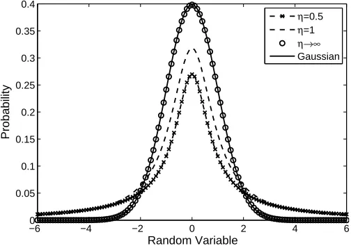
co-variance matrix and η > 0 is the number of degrees-of-freedom. As η → ∞ the Student t-distribution reduces to a Gaussian distribution. At finite values of η the Student distribution has heavier tails than the corresponding Gaus-sian for the same µ and Λ−1_{, and so the Student t-distribution represents a}

generalisation of the Gaussian distribution, Figure 1.

−6 −4 −2 0 2 4 6

0 0.05 0.1 0.15 0.2 0.25 0.3 0.35 0.4

Probability

Random Variable

η=0.5 η=1 η→∞ Gaussian

Figure 1: Univariate Student-tdistribution withµ=0 and Λ=1 for different values ofη. When

η→ ∞₍◦_{), the Student-tdistribution corresponds to a Gaussian distribution (solid line) and}

the two plots coincide.

Unfortunately, no closed-form solution exists when maximising the likeli-hood using a Student distribution. Thus an alternative representation of the Student distribution is required and this is given as an infinite mixture of scaled Gaussians, written as

T(x|µ,Λ−1, η) =

Z ∞

0

N(x|µ,(uΛ)−1)Ga(u|η/2, η/2) du (3)

In this paper, a novel mixture of experts model is introduced by using the Student-tdistribution, given in (3), for both the gate and expert functions. The gating function consists of a Student mixture model (SMM), while in the expert function the innovations take on the form of a Student distribution. This set up provides robustness to atypical data points in the dataset, both in the form of outliers in the output and non-Gaussian distributed inputs. The form of the MoE model used here is similar to the MoE model with Gaussian mixture model (GMM) at the gates, as given in [23, 16, 19]. However, as discussed in [27, 9], the GMM is susceptible to non-Gaussianity in the inputs and hence tends to select a more complex model (one which has more components) in order to capture the tails of the distribution. Naturally, this problem is inherited by the MoE when the gates take the form of GMM. Additionally, outliers in the observed variable will introduce bias in the regression, so using Student innovations helps to overcome poor regression [10].

2.2. Mixture of Experts Model LetX = [x1, . . . ,xN]⊤ ∈ RN×d

x

be adx _{dimensional input to the system}

of interest, consisting ofN data points, such that xn = [x1n, . . . , xd

x

n ]. Let the

corresponding vector of scalar outputs be y = [y1, . . . , yN]⊤ ∈ RN×1; then, a

regression MoE model withM experts is given by

yn= M

X

i=1

gi(xn, θgi)fi(xn,wi), (4)

wheregi(·) and fi(·) are theithgating and expert functions respectively. The

expert is restricted to be a vector function given by fi(xn,wi) = wi⊤[xn 1],

where wi are the expert weights which include a bias term given by the 1

appended to the input matrix. The gating function used here is a normalised Student-t function, such that

gi(xn, πi, θig, ηi) =

πiT(xn|µi,Λ−1i , ηi)

PM

l=1πlT(xn|µl,Λ−1l , ηl)

. (5)

whereθgi ={µi,Λi}. The mixing coefficients are given byπ={πi}Mi=1,

satisfy-ingπi≥0 andPMi=1πi= 1. Equation (5) can also be expressed using (3), such

that a latent scale variableuniis associated with each data pointxn and each

componenti. The likelihood for the MoE is represented as

p(yn|xn,Θ) = M

X

i=1

p(i|xn, πi, θgi, ηi)p(yn|xn, θei). (6)

p(i|xn, πi, θig, ηi) = gi(·) is the posterior conditional probability that xn is

as-signed to the segment corresponding to theith _{expert. The probability}

having meanfi given by

p(yn|xn, θie, κi) =T(yn|w⊤i [xn 1], τi−1, κi)

=

Z

N(yn|w⊤i [xn 1],(sniτi)−1)Ga(sni|κi/2, κi/2) dsni

(7)

The parameter vector for the experts is θe= [W,τ], whereW ={wi}Mi=1

is the weight vector, andτ−1={τ_i−1}M

i=1 is the variance. The set of unknown

model parameters in (6) is given byΘ= [π,η,κ,θg,θe]. The alternative model developed by [23] is adopted here in order to obtain closed form solutions for the parameter updates, and the joint density is given by

p(y,X|Θ) =

N

Y

n=1 M

X

i=1

πiT(xn|µi,Λ−i 1, ηi)

| {z }

˜ gi

T(yn|w⊤i [xn 1], τi−1, κi), (8)

where the gating network ˜gi is a Student Mixture Model (SMM). Maximum

likelihood estimation of SMM within the EM framework was introduced by [31], while a Bayesian approach using variational Bayes was tackled by [27, 9].

Discrete latent indicator variables Z = {zni}M,Ni=1,n=1 are introduced such

that if (xn, yn) was generated from the ith model thenzni= 1, otherwise it is

0. Thus the complete-data likelihood for (8) can be written as

p(y,X,Z,U,S|Θ) =

N

Y

n=1 M

Y

i=1

πiN(xn|µi,(uniΛi)−1)Ga(uni|ηi/2, ηi/2)×

N(yn|wi⊤[xn 1],(sniτi)−1)Ga(sni|κi/2, κi/2)

zni

,

(9)

where U, S are N ×M matrices, with U = [u1, . . . ,uN]⊤ = {uni}M,Ni=1,n=1,

whereun = [un1, . . . , unM], and similarly forS. Marginalising (9) over all the

latent variables,Θl _{= [Z,U,S], results in (8). Defining the likelihood in this}

way encourages soft competition such that only one expert is dominant in a certain region of the input space [14]. Following on from previous work in the literature, by maximising the marginal likelihood of the data, p(X,y|π,η,κ), updates for the mixing coefficientsπ [32, 19] and degree-of-freedom parameters

η and κ [27, 9] can be obtained. These parameters are denoted as ΘM L ₌

[π,η,κ], where the superscriptM Lrefers to the maximum-likelihood updating of the parameters. The rest of the parameters, θg and θe, and the latent variables are treated as random variables, and hence Bayesian inference is used to find approximate posterior distributions for these variables. An attractive advantage of using VBEM with the model described in this section is that [ΘV B_,Θl_{] = [{θ}g_,θe_},Θl_{] can be derived analytically and thus have closed-form}

3. Variational Bayesian Framework

Prior distributions for the random variables of the model’s parameters,ΘV B_,

are specified in Section 3.1. Details of the VBEM algorithm for the model described in this paper are given in Section 3.2. In Section 3.3 the optimised variational distribution update equations for all the random variables are given, while in Section 3.5 updates forΘM L_{are presented.}

3.1. Priors

Priors from the exponential family (example, Gaussian, Gamma and Wishart, where the Wishart is a multivariate version of the Gamma distribution) are considered in this work. These prior distributions are conjugate priors for the likelihood function given in (9), thus ensuring that the posterior distributions are of the same form as the prior. In this paper, the authors use the Gaussian distribution for parameters, the Gamma distribution for variance (since the variance is strictly positive) and the Wishart distribution for covariance (since covariance is the multivariate version of variance). More information regarding conjugate priors can be found in [33].

Since both the gating mean,µ, and precision,Λ, are assumed unknown, the conjugate prior assigned to these parameters for each Gaussian component is the Gaussian-Wishart prior,

p(µ,Λ) =p(µ|Λ)p(Λ)

=

M

Y

i=1

N(µi|m0,(β0Λi)−1)W(Λi|B0, ν0).

(10)

B0is adx_×dx_{symmetric, positive definite matrix, andν0> d}x_{−1 is the number}

of degrees-of-freedom of the Wishart distribution. The prior distribution of the joint weight and precision parameters for the expert function is given by a Gaussian-Gamma distribution,

p(W,τ|a) =

M

Y

i=1

N(wi|0,(τiAi)−1)Ga(τi|ρ0, λ0), (11)

where a = (a1, . . . ,aM), and ai = {ai,j}d

x₊₁

j=1 are the parameters associated

with automatic relevance determination (ARD) [34, 35]. If a−1_i,j = 0, then the corresponding input xj is irrelevant to form the distribution of the output yi

of the ith _{expert since the corresponding weight w}

i,j will be very small. The

matrixAi is formed from a such that Ai = diag(ai,1, . . . , ai,dx₊₁). a_i,j is the

hyperparameter on which the expert weightwi,j depends on and is given the

following hyperprior distribution

p(ai,j) =Ga(ai,j|c0, d0). (12)

priors. The joint distribution of all the random variables conditioned onΘM L

can be expressed hierarchically as,

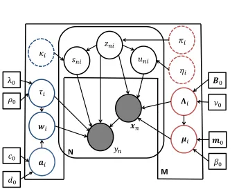
p(y,X,Θl,ΘV B,a|ΘM L) =p(X,y|Θl,Θ)p(Z|π)p(U|Z,η)p(S|Z,κ)

p(µ,Λ)p(W,τ|a)p(a), (13)

which is shown in Figure (2).

N

M

Figure 2: Graphical model for Bayesian MoE model with SMM gates and Student-texperts. The rounded plate denotesN i.i.d observations of yandX (shaded circles). The M-plate represents the M mixture components incorporating both the gate and expert parameters. The latent variables,Z, U and S, belong to both plates. Broken circles denote adjustable parameters, while square boxes refer to known hyperparameters. Unobserved random variables are indicated by complete circles (red corresponds to gate parameters, blue corresponds to expert parameters). The arrows represent conditional dependencies between the variables.

3.2. Variational Bayes Expectation Maximisation

byϑ, the log-marginal likelihood (denominator in Bayes theorem) is given by [36]

lnp(y) =F(q(ϑ)) + KL[q(ϑ)kp(ϑ|y)], (14) where KL[q(ϑ)k p(ϑ|y)] is the Kullback-Leibler (KL) divergence between the variational posterior distributionq(ϑ) and the true posteriorp(ϑ|y). Since the KL divergence is always positive, then F(q(ϑ)) is a lower bound of the log-marginal likelihood. The main objective of variational Bayes is to maximise F(q(ϑ)) with respect toϑin order to get a tight bound (hence minimising the KL divergence).

For the model specified in (9), the random variables areϑ= [Θl_,{ΘV B_,a}],

and thus constitutes both latent variables and model parameter variables. A constraint on the variational distribution is enforced; a factorised variational distribution is used in order to make evaluation of the lower bound tractable, that is,q(ϑ) =q(Θl_)q(ΘV B_{,a). The update equations, for the E- and M-steps,}

are obtained by performing functional differentiation ofF(q(ϑ)) with respect to

q(Θl_{) andq(Θ}V B_{,a) respectively, and equating it to zero. At thek}th _iteration

the two steps are given by [29],

VBE-step: lnq(Θl₎ k+1∝

Z

q(ΘV B_,a)

klnp(y,X,Θl|Θ)dΘV Bda

∝Eq(ΘV B_,a)_k[lnp(y,X,Θ

l_|Θ)].

(15)

VBM-step: lnq(ΘV B,a)k+1∝lnp(ΘV B,a) +

Z

q(Θl)k+1lnp(y,X,Θl|Θ)dΘl

∝lnp(ΘV B,a) +Eq(Θl₎

k+1[lnp(y,X,Θ

l_|Θ)],

(16)

wherep(y,X,Θl_{|Θ) is given by the complete-data likelihood in (9), andΘ =}

[ΘV B_,ΘM L_{]. E}

q(·) is the expectation with respect to the corresponding

varia-tional distribution, andp(ΘV B,a) is the prior over the model parameters which are specified in Section 3.1. The lower bound is maximised by iteratively using the update equations given in (15) and (16) until convergence. However, conver-gence to the global maximum is not guaranteed and several runs with different initial conditions need to be considered to overcome this problem.

3.3. Variational Inference

A VBEM algorithm for the SMM was considered in [27], where a factorised form was assumed between the indicator variables Z and scale variables U. The restriction of having a factorised form for the latent random variables was removed in [9] where the authors considered correlations between these two random variables. The approach used here follows that given in [9] since it underestimates less the variance in the posterior distribution. The factorised variational distribution for the MoE model described in this paper, is expressed as,

The functional form of the variational distributions will be the same as the priors, and this is a consequence of adopting conjugate priors for the model structure. The optimal variational distributions are noted below, and expressed asq∗_{(·). The VBM-step uses (16) to update the variational distributions of the}

model parameters and these are shown in equations (18)-(24). The variational update equations for the latent variablesZ, U and S in the VBE-step, using (15), are shown in equations (25)-(31).

The joint variational distribution of the gate mean and covariance is a Gaussian-Wishart distribution, given by

q∗

(µi,Λi) =N(µi|mi,(βiΛi)−1)W(Λi|Bi,νi), (18)

where

mi=

β0m0+PNn=1E[zni]E[uni]xn βi

, βi =β0+ N

X

n=1

E[zni]E[uni]

Bi−1=B0−1+ N

X

n=1

E[zni]E[uni]xnx⊤n +β0m0m ⊤

0 −βimim⊤i

νi=ν0+Ni , Ni= N

X

n=1

E[zni].

(19)

The joint variational distribution of the expert functions’ mean and variance is a Gaussian-Gamma distribution having the following form

q∗

(wi, τi) =N(wi|wˆi,Ψi)Ga(τi|ρi, λi), (20)

where

ˆ

wi=Li[X 1]⊤Viy

Li= ([X 1]⊤Vi[X 1] + Υi)−1

Vi= diag(E[z1i]E[s1i], . . . ,E[zN i]E[sN i])

Ψi= λi ρi

Li

ρi=ρ0+ 0.5Ni , λi=λ0+ 0.5Ri

Ri= (y−[X 1] ˆwi)⊤Vi(y−[X 1] ˆwi) + ˆw⊤i Υiwˆi .

(21)

The term Υi =Ea_i[Ai] is defined in (24). The variational distribution for the ARD parameters is

q∗(ai,j) =Ga(ai,j|ci, di,j), (22)

where

ci=c0+ 0.5, di,j =d0+ 0.5ξi,j

ξi,j= ρi λi

ˆ

where (Li)j,j is thejthdiagonal element ofLi, andwˆi={wˆi,j}d

x₊₁

j=1 . Using the

statistic of a mean from a Gamma distribution, then

Υi=Ea_i[Ai] = diag

_c

i di,1, . . . ,

ci di,dx₊₁

. (24)

The VBE-step consists of updating the variational distribution ofZ,U andS. The relevant equations are listed below, and the full derivation can be found in Appendix A. The variational distribution for the latent indicator variables follows a multinomial distribution, such that

lnq∗(Z) =

N X n=1 M X i=1

znilnrni and rni= γni

PM l=1γnl

, (25)

whereE[zni] =rni, and once the scale variablesUandShave been marginalised

out gives

γni=

Γηi+dx

2

Γ(0.5ηi)(ηiπ)0.5dx πiΛˆ0i.5

̟ni ηi

+ 1

!−ηi+dx 2

× Γ

κi+1

2

Γ(0.5κi)(κiπ)0.5

ˆ

τ0.5 i

ξni κi

+ 1

!−κi+1 2

.

(26)

The first part of (26) comprises the contribution of the gate, while the second part is due to the expert parameters. Both parts form individual weighted Student-tdistributions. The required statistics are,

ln ˜Λi=E[ln|Λi|] = dx X

j=1 ψ

_ν

i+ 1−j

2

+ ln|Bi|,

ln ˜τi=E[lnτi] =ψ(ρi)−ln(λi),

(27)

where ψ(·) is the digamma function, and ̟ni andξni are given in (Appendix

A.3) and (Appendix A.6) respectively. The variational distribution for the scale variablesU andS follow Gamma distributions. These are given by

q∗

(uni|zni= 1) =Ga(uni|αuni, ǫuni), (28)

where

αuni=

dx+ηi

2 , ǫ

u ni=

̟ni+ηi

2 . (29)

Similarly forS,

q∗

(sni|zni= 1) =Ga(sni|αnis , ǫsni), (30)

where

αsni=

1 +κi

2 , ǫ

s ni=

ξni+κi

2 . (31)

those obtained in the MoE with Gaussian gates and experts with the exception that now some of the equations depend onE[uni] andE[sni], and so derivations

are not given here but can be found in [19]. Details regarding the VBE-step can be found in Appendix A. The equations are coupled, and therefore need to be iterated until convergence. However, some of the above equations also require the parametersπ,ηandgto be known. Estimation of these parameters is dealt with in the following sections.

3.4. Variational Lower Bound

The quantities needed to evaluate the variational lower bound (VLB),F(q(ϑ)), are obtained from the functional forms of the variational distributions calculated in the previous section. Interested readers are referred to [29] for a derivation of the VLB as expressed below. The VLB for the mixture of experts model is

F(q) =Eq

lnp(y,X,Z,U,S,µ,Λ,W,τ,a|ΘM L)−Eq[lnq(Z,U,S,µ,Λ,W,τ,a)]

=Eq

lnp(y,X,Z,U,S|ΘM L,ΘV B)+Eq[lnp(µ,Λ)] +Eq[lnp(W,τ|a)] +Eq[lnp(a)]

−Eq[lnq∗(Z,U,S)]−Eq[lnq∗(µ,Λ)]−Eq[lnq∗(W,τ)]−Eq[lnq∗(a)] ,

(32)

where theEq refers to the expectation with respect to the variational

distribu-tionq∗

(Z,U,S,θg,θe,a). This lower bound approximates the true marginal log-likelihood when convergence is reached. The specific expression for the lower bound is given in Appendix B.

3.5. Optimisingπ,η andκvia Maximum Likelihood

By maximising the variational lower bound with respect to the parameter of interest, a corresponding update equation can be obtained. Taking the deriva-tive of (Appendix B.1) with respect to the mixing coefficients (only this term is dependent onπ, all the other terms can be ignored) and setting it to zero, gives [32]

πi=

1

N N

X

n=1

rni. (33)

Maximising the mixing coefficients in this way ensures that any surplus experts will haveπi →0. Thus the number of experts can be set large and any excess

experts can be eliminated from the model. The degree-of-freedom parameterηis also found by maximising the expression obtained in (32), specifically (Appendix B.2). However, this results in the nonlinear equation

lnηi

2 + 1−ψ

_ηi

2

+ 1

Ni N

X

n=1

rni{E[lnuni]−E[uni]}= 0, (34)

which requires a line search algorithm to solve forηi. In order to reduce

Stirling’s series for ln Γ(·) [37]. This gives

ηi= ₁ 1 Ni

PN

n=1rni{E[uni]−E[lnuni]} −1

. (35)

Similarly forκ(using Stirling’s series and differentiating (Appendix B.3)) gives

κi=

1

1 Ni

PN

n=1rni{E[κni]−E[lnκni]} −1

. (36)

Approximate solutions for updating the degree-of-freedom parameter has been applied successfully in [38] using a direct approximate formula and in [7] us-ing Stirlus-ing’s series. The derivation for (35) (and consequently (36)) is found in Appendix C. All the above equations are required for evaluation of some of the expressions obtained in Section 3.3, and so these update equations are interleaved into the iterative procedure.

3.6. Posterior Predictive Distribution

In order to perform predictions of the output to an unseen inputxN+1, the

posterior predictive distribution needs to be evaluated. The posterior predictive distribution is given byp(yN+1|xN+1,D), whereD= [y,X] is the training data.

This distribution is obtained by marginalising the product of the likelihood and the parameter posterior distribution with respect to the parameters. The predictive distribution is similar to that obtained for MoE with GMM gates ans experts, see [16, 19] for proofs, with the exception that now the scale variable

snialso appears in the expression.

In order to obtain an analytical solution for the predictive distribution,sni

cannot be marginalised out, so its maximum-a-posteriori (MAP) estimate is used instead (obtained from (30) and (31)). Lettingn′

=N+ 1, the predictive distribution is given by

p(yn′|xn′,D) =

M

X

i=1 φn′,i

T

yn′

wˆ

⊤ i [xn′ 1],

ρisMAPn′_i

λi

(1 +sMAPn′i [xn′ 1]Li[xn′ 1]

⊤

)−1,2ρi

,

(37)

where{φn′,i}Mi=1 take value 1 with probabilities{gi(xn′, πi, θg_iMAP)}Mi=1

respec-tively (using (5) at the maximum a posteriori (MAP) estimatesθ_MAPg ={µMAP,ΛMAP}

obtained from the posterior distribution (18), and the final value forπ). At any given timen′

only one {φn′,i}Mi=1 can be 1 (the rest are zero) corresponding to

the gate with the largest probability. The relevant statistics for prediction are

E[yn′] =

M

X

i=1

and

Var[yn′] =

M

X

i=1

φn′,iλi(1 +s MAP

n′i [xn′ 1]Li[xn′ 1]⊤)

sMAP n′i (ρi−1)

. (39)

In the event that no outliers are present, then the Student-t distribution at the gates and experts will reduce to a Gaussian distribution, and the posterior predictive distribution will be the same as in [19]: κi→ ∞and so sMAPn′i →1.

Algorithm 1: VBEM algorithm for robust MoE

Initialise the hyperparameters for Student-t gates, m0,β0,B0 andν0.

Initialise the hyperparameters for linear expertsρ0,λ0, c0, d0 and Υ(0)i = dc00Idx+1 ∀i.

Initialiseκ(0)_ni =η(0)_ni = 1 and γ_ni(0) ∼ U[0,1]∀i, n.

fork= 0 : stopping criteria (k′

) = (k+ 1)

1. Evaluate mixing coefficientsπ(k′)via (33).

2. Update the gate parametersm(ik′), β (k′₎

i , ν (k′₎

i , B −1(k′₎

i via (19).

3. Update the expert parameters ˆw(_ik′), Ψ_i(k′), ρ_i(k′), λ(_ik′)via (21).

4. Update ARD parametersc(ik′), d (k′₎

i,j via (23).

5. Update forγ(_nik′)of variational distribution ofZ via (26).

6. Update for parameters of variational distribution ofU via (29).

7. Evaluate degree-of-freedom parameterη(k′)via (35).

8. Update for parameters of variational distribution ofS via (31).

9. Evaluate degree-of-freedom parameterκ(k′₎

via (36).

end for

4. Results

In this section, the MoE model with Student-tgates and experts is compared to the MoE model with Gaussian gates and experts (details of this algorithm can be found in [19]) on two datasets: a simulated Duffing oscillator and the Z24 bridge data. For brevity, the two different modelling techniques are referred to as S-MoE and G-MoE respectively. Outliers are artificially added to both datasets in order to show that when outliers are present in the training data, assuming a Gaussian form will result in a biased regression model and/or a more complex model.

way so as to define a large covariance (hence a low precision) with respect to the data so as to avoid confining each Gaussian gate to its local cluster, and these were set differently for the two examples (details given in the following sections). The hyperparameterm0, the centre of the gate clusters, was set to zero. Broad priors were assigned to the expert hyperparameters, given byρ0 =c0 = 0.01 andλ0=d0= 1e−4_.

Convergence of the algorithm is achieved by monitoring changes in the vari-ational lower bound (32). The algorithm is stopped when the change in VLB between iterations falls below a certain threshold. In order to overcome the problem of local maxima in the VLB distribution, Algorithm 1 was run for 100 instances withγ_ni(0) initialised randomly for each run: values were drawn from a Uniform distribution between 0 and 1 (represented as U[0,1] in Algorithm 1). The model with the largest VLB was selected as being the model that best represents the data.

As already mentioned in Section 3.5, the number of experts,M, needs to be initialised to a large number (here, the term ’large’ is relative and depends on the data under investigation), and any mixing coefficient that converges to zero results in its corresponding expert not contributing to the model output. The authors investigated the effect of this initialisation by running the algorithm for different initial values forM; the final results obtained were similar for all cases. In this work, the number of experts was set to 6 for the examples considered in this section, and any πi <10−5 resulted in the corresponding expert to be

removed from the final model. The choice ofM depends on the data and it is up to the modeller to set. Alternatively, rather than setting a generic threshold; the experts which contribute to the output can be determined, then remove the surplus experts. Here a generic threshold was set in advance.

4.1. The Duffing Oscillator

The nonlinear Duffing oscillator, consisting of a mass, linear and nonlinear springs and a damper, is a classic example used for system identification in dynamics. The values of parameters used here arem= 1,k= 104_{,k3= 5×10}9

andc= 20 respectively. The differential equation, given by

my¨+cy˙+ky+k3y3=Pcos(ωt), (40)

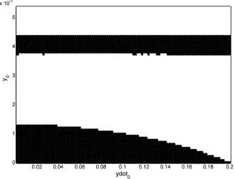
amplitudes, including a curved bifurcation front, as seen in Figure 3. Modelling these bifurcations has been tackled using treed Gaussian processes [40] and later extended to G-MoE models in order to model splits in the data that are not parallel to the input variables [19]. In this paper, the effect of outliers on the modelling process is investigated, and outliers are artificially added to the data. The aim here is to fit a MoE model to the response surface of the system, such that it is capable of capturing all the bifurcations accurately, whilst also being insensitive to outliers.

Figure 3: Top-down view representation of response surface for amplitude variation: multiple bifurcations are present between low amplitude (black) and high amplitude (white) as the initial displacement (y0) and velocity (ydot0) of the mass are varied.

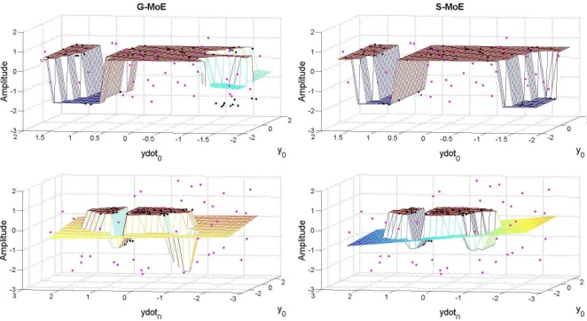
output only (these represent data points which could not have been generated by the process), while the second case deals with outliers in both the inputs and the output (representing the situation of when the true underlying system is masked by noise). The G-MoE and S-MoE models were trained using this dataset.

The results obtained from the G-MoE and S-MoE algorithms are shown in the left and right hand plots respectively in Figure 4; the top row represents the surface plot generated when outlier points (pink scatter points) are restricted to the output variable, while the bottom row shows the effect of expanding the range of outlier points. The S-MoE model (left column) provides a more accu-rate predictive response surface than the G-MoE model (right column) for two reasons: firstly, the model captures all of the bifurcations, and secondly, the model is capable of providing accurate predictions because each expert repre-sents the black scatter points (system data). Thus the S-MoE model appears to be insensitive to the outliers present in the training data. The bottom right plot shows that outlier points outside the region of interest are assigned the same expert, and an accurate model for the bifurcations and system data points is still obtained. The use of a Student-tdistribution is now effective since κi <1

for all the dominant experts, thus the heavier tails ensure robustness in the regression analysis.

On the other hand, the G-MoE model performs additional splits to the data providing a more complex and incorrect model which does not capture the cor-rect bifurcations. In addition, the G-MoE with outliers fails to provide accurate regression modelling since it does pass thorough the black scatter points, which represent the system. The G-MoE fails to capture the true underlying model since the predictive surface plot is highly influenced by outliers. Thus, the S-MoE algorithm is superior to the G-S-MoE model in the presence of outliers, providing a simpler more accurate model than the G-MoE model counterpart.

4.2. Z24 Bridge Data

The Z24 bridge was a bridge in Switzerland that prior to its demolishment in the late 1990s was under intense monitoring by the ’SIMCES project’ [41]. The modal parameters of the bridge were tracked, and realistic damage scenarios were gradually introduced. Environmental factors were also measured, such as air temperature, soil temperature and humidity among several other variables. The Z24 bridge has been well studied within the structural health monitoring (SHM) community in order to establish detection of damage independently of environmental factors [42, 43].

Figure 4: Comparison of the G-MoE model (left hand column) and S-MoE model (right hand column). The top row represents the surface response plot for the case when outliers are present in the output only, while the bottom row deals with the situation when outliers are present in both the inputs and output. The mesh represents the mean predictive surface plot, with the scatter points representing the training data: black points are underlying system while pink points are the artificially added outliers. The S-MoE model captures the underlying system by accurately modelling the black scatter points, whilst the G-MoE is highly influenced by outliers and hence fails to model the black scatter points. Note that the axes represent the normalised data.

temperature variation only. This dataset was analysed using treed GPs [44] and G-MoE [19] since a bilinear relationship exists between the air tempera-ture and the natural frequency of the bridge. Using models that are capable of automatically switching between different regimes are important for modelling and understanding the underlying physics governing the system. The aim of the modelling procedure is to obtain a model that is dependent on temperature only. The model obtained using this training dataset is then tested on data that contains both temperature changes and damage effect. When predictions are performed on the damaged section, the model should be capable of giving an indication that other factors besides temperature are affecting the modal fre-quency. Within a Bayesian setting the variance of the predicted signal can be calculated naturally, and hence credible bounds can be computed. Damage is detected when the measured signal deviates significantly from the predictions, which can be determined when the signal moves outside the credible intervals. Switching models, on this dataset, outperformed standard GP models with re-spect to determining damage detection [44].

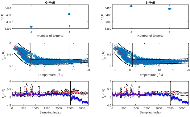
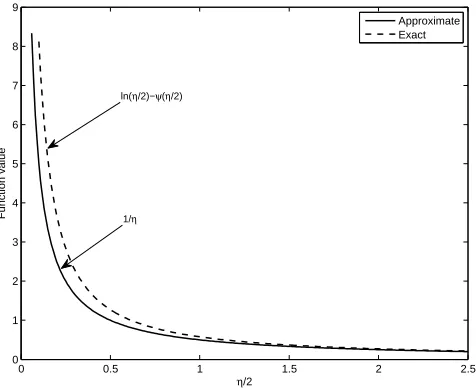
(34), is used since Stirling’s approximation tends to underestimate the variance (see Appendix C) causing tighter bounds. The expression obtained in (34) can be solved in Matlabr_{using thefzerofunction. The dataset is first run with no}

outliers, and the results are shown in Figure 5. The plots in the top row show the variational lower bound versus the number of experts in the final models obtained using 100 random runs. The S-MoE model achieves a tighter bound (larger VLB value) with a less complex structure (2 experts versus the 3 experts needed by the G-MoE model). Note, how for the S-MoE, models with 3 experts achieved a lower VLB than the models with 2 experts because complexity is naturally penalised within a Bayesian framework. The G-MoE has splits at 0.375◦_{C and 13.4}◦_{C, while the S-MoE requires one split at 0.84}◦_{C. Thus both}

models have a split close to 0◦_{C, however the S-MoE has a less complex structure}

since it combines two experts into one (and the degree-of-freedom parameters for this component have very low values for both the gate and expert). Both models are capable of detecting damage in the bridge since the second natural frequency values quickly move outside the credible bounds of the model (Figure 5, bottom row).

2 3

Number of Experts 8360

8380 8400 8420

VLB

G-MoE

-5 0 5 10 15 20 Temperature ( °_C)

5 5.5 6

f2

(Hz)

0 500 1000 1500 2000 2500 3000 Sampling Index

4.5 5 5.5 6

f2

(Hz)

2 3

Number of Experts 8360

8380 8400 8420

VLB

S-MoE

-5 0 5 10 15 20 Temperature ( °_C)

5 5.5 6

f2

(Hz)

0 500 1000 1500 2000 2500 3000 Sampling Index

4.5 5 5.5 6

f2

(Hz)

Figure 5: Comparison of the G-MoE model (left hand column) versus the S-MoE model (right hand column) on the Z24 dataset when no outliers are present. The top row shows the variational lower bound versus number of experts. In order enhance the visualization of the results, a small amount of uniform noise has been added to the horizontal position of the points. The middle row shows the relationship of the second natural frequency with temperature: blue scatter points represent the training data, the red line represents the model mean and the black lines represent±_{99% credible intervals. The black vertical lines indicate}

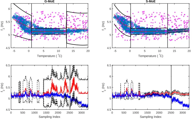
Outlier points are artificially added to the Z24 bridge data, numbering 15% of the original training dataset. The outliers were randomly drawn from a uniform distribution along the input and the output ranges. Figure 6 shows the results obtained when the G-MoE and S-MoE algorithms are run on this new dataset. It is immediately obvious that the G-MoE model fails to represent the data very accurately since the regression is severely affected by the outliers. In particular the variance of the predicted output is very wide in order to accommodate the outliers (since it is highly influenced by outlier points). As a consequence, the G-MoE model is incapable of detecting damage to the bridge due to a very wide variance associated with the predictions, such that the credible intervals now enclose the measured modal frequency of the test set, as shown in the left bottom plot in Figure 6. On the other hand, the S-MoE successfully captures the dynamics of the system having splits at 0.21◦_{C and 12.7}◦_{C (the model has}

-5 0 5 10 15 20 Temperature ( °_C)

4.5 5 5.5 6

f2

(Hz)

G-MoE

0 500 1000 1500 2000 2500 3000 Sampling Index

4.5 5 5.5 6 6.5

f2

(Hz)

-5 0 5 10 15 20 Temperature ( °_C)

4.5 5 5.5 6

f2

(Hz)

S-MoE

0 500 1000 1500 2000 2500 3000 Sampling Index

4.5 5 5.5 6 6.5

f2

(Hz)

Figure 6: Comparison of the G-MoE model (left hand column) versus the S-MoE model (right hand column) on the Z24 dataset when 15% outliers are added. The top row shows the relationship of the second natural frequency with temperature: blue scatter points represent the training data, pink scatter points are the artificially added outliers, the red line represents the model mean and the black lines represent±_{99% credible intervals. The black vertical lines}

indicate the different expert regions assigned by the corresponding models. The bottom row plots are the predictions of the models (red) on the test data (blue), where the black dashed line represents the±_{99% credible intervals. The black vertical line indicates start of damage.}

5. Conclusions

Acknowledgement

Author T. Baldacchino would like to thank the Leverhulme Trust Research Project Grant for financial support. The authors would like to acknowledge Dr. Elizabeth J. Cross, from the University of Sheffield, for providing access to the Z24 bridge data.

Appendix A. Derivation of lnq(Z, U , S)

The joint distribution over the latent variables is given by

lnq∗

(Z,U,S) =E[lnp(y,X,Z,U,S,ΘV B,a)|ΘM L] =E[lnp(y,X,Z,U,S|ΘV B,ΘM L] +C

∝

N

X

n=1 M

X

i=1 zni

E[ln{πiN(xn|µi,(uniΛi)−1)Ga(uni|ηi/2, ηi/2)}]

| {z }

lnP1

+E[ln{N(yn|[xn 1]wi,(sniτi)−1)Ga(sni|κi/2, κi/2)}]

| {z }

lnP2

,

(Appendix A.1)

whereCcontains terms independent ofZ,U,S. Concentrating on the first part of the right hand side of the equation (lnP1), and expanding the terms gives,

lnP1 = lnπi−0.5dxln(2π) + 0.5 ln ˜Λi−ln Γ(0.5ηi) + ηi

2 ln

ηi

2 + 0.5dxlnuni−0.5uni̟ni−(ηi

2 −1) lnuni−

ηi

2uni ,

(Appendix A.2)

where

̟ni= Tr(E[Λi]E[(xn−µi)(xn−µi)⊤])

=νi(xn−mi)Bi(xn−mi)⊤+βi−1dx ,

(Appendix A.3)

and the expectation E[·] is taken according to the variational posterior distri-bution of that parameter. In order to marginalise out the scale variablesuni

in order to compensate for this marginalisation results in

lnP1 = lnπi+ 0.5 ln ˆΛi+ lnGa

uni

ηi+dx

2 ,

̟ni+ηi

2

−ηi+d

x

2 ln

̟ni+ηi

2

−0.5dxln(2π) + ln Γηi+d

x

2

−ln Γ(0.5ηi) + ηi

2 ln

ηi

2

= lnπi+ 0.5 ln ˆΛi+ lnGa

uni

ηi+dx

2 ,

̟ni+ηi

2

−ηi+d

x 2 ln ηi 2 ̟ni ηi + 1 ! −d x

2 ln(2π) + ln Γ

_ηi+dx

2

−ln Γ(0.5ηi) + ηi

2 ln

ηi

2

= lnπi+ 0.5 ln ˆΛi+ lnGa

uni

ηi+dx

2 ,

̟ni+ηi

2

−ηi+d

x 2 ln ̟ni ηi + 1 !

+ ln Γηi+d

x

2

−ln Γ(0.5ηi)− dx

2 ln(ηiπ) Taking the exponential of the above equation gives

P1 =

Γηi+dx

2

Γ(0.5ηi)(ηiπ)0.5dx πiΛˆ0i.5

̟ni ηi

+ 1

!−ηi+dx 2

Gauni

ηi+dx

2 ,

̟ni+ηi

2

,

(Appendix A.4) where the first part is a weighted Student-tdistribution. Similarly, for the part contributed by the expert (P2) gives

P2 =

Γκi+1

2

Γ(0.5κi)(κiπ)0.5

ˆ

τi0.5 ξni

κi

+ 1

!−κi+1 2

Gasni

κi+ 1

2 ,

ξni+κi

2

,

(Appendix A.5) where

ξni=E[τi](yn−[xn 1]E[wi])2

= ρi

λi

(yn−[xn 1] ˆwi)2+ [xn 1]Li[xn 1]⊤ .

(Appendix A.6)

Using (Appendix A.4) and (Appendix A.5) and substituting into (Appendix A.1), gives the posterior variational distribution for lnq∗_(Z,

U,S). Hence,

q∗₍

Z) is obtained by marginalising this expression over U and S, and noting that the integral of a Gamma distribution is 1 then this proves the expression forγniin (26). This variational distribution needs to be normalised, and this is

given as

lnq∗

(Z) =

N X n=1 M X i=1

znilnrni, (Appendix A.7)

withrni=γni/Plγnl. Equation (Appendix A.7) follows from the fact that for

each value ofn, the quantitieszni are binary andPizni= 1. Since (Appendix

A.7) is a multinomial distribution, then it follows thatE[zni] =rni. The

vari-ational distribution of the scale variablesuni andsniare given by the Gamma

Appendix B. Variational Lower Bound

The expressions for the individual terms in (32) are given here. Letting ln ˆAi=E[ln|Ai|] = Pd

x₊₁

j=1 (ψ(ci)−lndi,j), ln ˆuni=E[lnuni] =ψ(αuni)−lnǫuni

and ¯uni=E[uni] =αuni/ǫuni(and similarly for the latent variables sni), then:

Eq[lnp(y,X|Z,U,Θ)] =

1 2 N,M X n,i rni n

−dxln 2π+dxln ˆuni+ ln ˆΛi−u¯ni̟ni

−ln 2π+ ln ˆτi+ ln ˆsni−s¯niξni}

where̟niandξniare given in (Appendix A.3) and (Appendix A.6) respectively.

Eq[p(Z|π)] =

N,M

X

n,i

rnilnπi (Appendix B.1)

Eq[p(U|Z,η)] =

N,M X n,i rni ( ηi 2 ln ηi

2 −ln Γ(

ηi

2) +

ηi

2 −1

!

ln ˆuni− ηi

2u¯ni

)

(Appendix B.2)

Eq[p(S|Z,g)] =

N,M X n,i rni ( κi 2 ln κi

2 −ln Γ(

κi

2 ) +

κi

2 −1

!

ln ˆsni− κi

2 ¯sni

)

(Appendix B.3)

Eq[p(µ,Λ|a)] =

M X i=1 1 2

−dx_{ln 2π+d}x_{lnβ0+ ln ˆΛ}

i−νiβ0(mi−m0)⊤Bi(mi−m0)− β0 βi

dx

+2 lnCW(B0, ν0) + (ν0−dx−1) ln ˆΛi−νiTr(B0−1Bi)

o

Eq[p(W,τ)] =

M X i=1    1 2 

−dxln 2π+ (dx+ 1) ln ˆτi+ ln ˆAi− dx₊₁

X j=1 ci di,j ρi λi ˆ

w⊤i wˆi+ (Li)j,j

!



−ln Γ(ρ0) +ρ0lnλ0+ (ρ0−1) ln ˆτi−λ0ρi λi

Eq[p(a)] =

M,dx₊₁ X

i,j

−ln Γ(c0) +c0lnd0+ (c0−1)(ψ(ci)−lndi,j)−d0 ci di,j

The remaining terms in (32) are the entropies of the corresponding variational distributions, such that:

Eq[q(Z)] =

N,M

X

n,i

rnilnrni

Eq[q(U|Z)] =

N,M

X

n,i

rni{−ln Γ(αuni) + (αuni−1)ψ(αuni) + lnǫuni−αuni}

Eq[q(S|Z)] =

N,M

X

n,i

rni{−ln Γ(αsni) + (αsni−1)ψ(αsni) + lnǫsni−αsni}

Eq[q(µ,Λ)] =

M

X

i=1

1 2

n

dxlnβi−dx(1 + ln 2π) + 2 lnCW(Bi, νi) + (νi−dx) ln ˆΛi−dxνi

o

Eq[q(W,τ)] =

M

X

i=1

1 2[(d

x_{+ 1) lnτ}

i+ ln|Li| −(dx+ 1)(1 + ln 2π)]

−ln Γ(ρi) + (ρi−1)ψ(ρi) + lnλi−ρi}

Eq[q(a)] =

M,dx₊₁ X

i,j

{−ln Γ(ci) + (ci−1)ψ(ci) + lndi,j−ci}

whereCW(·) is the normalisation constant associated with the Wishart distribu-tion. The expressions above can be combined to simplify the overall variational lower bound expression.

Appendix C. Stirling’s Series

The derivation for expressions (35) and (36) is given here. The Gamma function can be approximated using Stirling’s series, and a truncated version of Stirling’s series is given by [37]

ln Γ(η 2)≈

1

2ln 2π+ (

η

2 − 1 2) ln

η

2 −

η

Substituting (Appendix C.1) into (Appendix B.2), and differentiating with re-spect toη gives

d dηi N X n rni ( 1 2ln ηi 2 − 1

2ln 2π+

ηi

2 +

ηi

2 −1

!

ln ˆuni− ηi

2u¯ni

) = 0 1 2 N X n rni ₁

ηi + 1 + ln ˆuni

−u¯ni

= 0

Ni ηi

+Ni− N

X

n

rni(¯uni−ln ˆuni) = 0

ηi=

1

1 Ni

PN

n rni(¯uni−ln ˆuni)−1

Comparing this equation to the exact equation given in (34), results in lnηi 2 −

ψ(ηi

2) being approximated by 1

ηi

. The plot of these two functions is given in

Figure (C.7), and it can been seen that the function plots differ for low values of

η, with the approximate solution underestimating the value ofη. Asηincreases, the two functions converge. The same procedure is used to obtain (36).

0 0.5 1 1.5 2 2.5

0 1 2 3 4 5 6 7 8 9 Function value η/2 Approximate Exact 1/η

ln(η/2)−ψ(η/2)

Figure C.7: A plot comparing the approximate solution using Stirling’s series and the exact solution given by (34).

[2] V. Barnett and T. Lewis.Outliers in Statistical Data (Third Edition). John Wiley and Sons, 1994.

[3] Jason W. Osborne and Amy Overbay. The power of outliers (and why researchers should always check for them). Practical Assessment, Research & Evaluation, 9(6), 2004.

[4] M. West. Robust sequential approximate Bayesian estimation. Journal of the Royal Statistical Society. Series B (Methodological), 43(2):157–166, 1981.

[5] Kenneth L. Lange, Roderick J. A. Little, and Jeremy M. G. Taylor. Ro-bust statistical modeling using thet distribution.Journal of the American Statistical Association, 84(408):881–896, 1989.

[6] Jarno Vanhatalo, Pasi Jyl¨anki, and Aki Vehtari. Gaussian process regres-sion with Student-t likelihood. InConference on Neural Information Pro-cessing Systems (NIPS), 2009.

[7] Jacqueline Christmas and Richard Everson. Robust autoregression: Student-t innovations using variational Bayes. IEEE Transactions on Sig-nal Processing, 59(1):48–57, 2011.

[8] Johan Dahlin, Fredrik Lindsten, Thomas B. Sch¨on, and Adrian Wills. Hi-erarchical Bayesian approaches for robust inference in ARX models. InThe 16th IFAC Symposium on System Identification, 2012.

[9] C´edric Archambeau and Michel Verleysen. Robust Bayesian clustering. Neural Networks, 20:129–138, 2007.

[10] Weixin Yao, Yan Wei, and Chun Yu. Robust mixture regression using the t-distribution. Computational Statistics and Data Analysis, 71:116–127, 2014.

[11] C. S. Wong and W. S. Chan. A Student t-mixture autoregressive model with applications to heavy-tailed financial data.Biometrica, 96(3):751–760, 2009.

[12] F. Chamroukhi. Robust mixture of experts modeling using thet distribu-tion. Neural Networks, 2016.

[14] Robert A. Jacobs, Michael I. Jordan, Steven J. Nowlan, and Geoffrey E. Hinton. Adaptive mixtures of local experts. Neural Computation, 3:79–87, 1991.

[15] Steve Waterhouse, David MacKay, and Tony Robinson. Bayesian meth-ods for mixture of experts. In David S. Touretzky Michael C. Mozer and Michael E. Hasselmo, editors, Advances in Neural Information Processing Systems, volume 8, pages 351–357. MIT Press, 1996.

[16] Naonori Ueda and Zoubin Ghahramani. Bayesian model search for mixture models based on optimizing variational bounds.Neural Networks, 15:1223– 1241, 2002.

[17] Christopher M. Bishop and Markus Svens´en. Bayesian hierarchical mixture of experts. In Uncertainty in Artificial Intelligence: Proceedings of the Nineteenth Conference, 2003.

[18] Alexandre X. Carvalho and Martin A. Tanner. Modeling nonlinearities with mixtures-of-experts of time series models. International Journal of Mathematics and Mathematical Sciences, 2006, 2006.

[19] Tara Baldacchino, Elizabeth J. Cross, Keith Worden, and Jennifer Rowson. Variational Bayesian mixture of experts models and sensitivity analysis for nonlinear dynamical systems. Mechanical Systems and Signal Processing, Under Review.

[20] Michael I. Jordan and Robert A. Jacobs. Hierarchical mixtures of experts and the EM algorithm. Neural Computation, 6:181–214, 1994.

[21] Fengchun Peng, Robert A. Jacobs, and Martin A. Tanner. Bayesian in-ference in mixtures-of-experts and hierarchical mixtures-of-experts models with an application to speech recognition. Journal of the American Statis-tical Association, 91(435):953–960, 1996.

[22] Seniha Esen Yuksel, Joseph N. Wilson, and Paul D. Gader. Twenty years of mixture of experts. IEEE Trans. Neural Netw. Learning Syst., 23(8):1177– 1193, 2012.

[23] Lei Xu, Michael I. Jordan, and Geoffrey E. Hinton. An alternative model for mixtures of experts. In J.D. Cowan, G. Tesauro, and J. Alspector, editors, Advances in Neural Information Processing Systems, pages 633–640. MIT Press, 1995.

[25] Carl Edward Rasmussen and Zoubin Ghahramani. Infinite mixtures of Gaussian process experts. In Advances in Neural Information Processing Systems 14 (NIPS), pages 881–888, 2002.

[26] C. Yuan and C. Neubauer. Variational mixture of Gaussian process experts. In Advances in Neural Information Processing Systems (NIPS) 21, pages 1897–1904, 2009.

[27] Markus Svens´en and Christopher M. Bishop. Robust Bayesian mixture modelling. Neurocomputing, 64:235–252, March 2005.

[28] H´ector Allende, Romina Torres, Rodrigo Salas, and Claudio Moraga. Ro-bust learning algorithm for the mixture of experts. InPattern Recognition and Image Analysis, Lecture Notes in Computer Science, volume 2652, pages 19–27, 2003.

[29] Matthew J. Beal and Zoubin Ghahramani. The variational bayesian EM algorithm for incomplete data: with application to scoring graphical model structures. In Jos´e M. Bernardo, M. J. Bayarri, A. Philip Dawid, James O. Berger, D. Heckerman, A. F. M. Smith, and Mike West, editors,Bayesian Statistics 7. Oxford University Press, 2003.

[30] Chuanhai Liu and Donald B. Rubin. ML estimation of thet distribution using EM and its extensions, ECM and ECME. Statistica Sinica, 5:19–39, 1995.

[31] D. Peel and G.J. McLachlan. Robust mixture modelling using thet distri-bution. Statistics and Computing, 10:339–348, 2000.

[32] Adrian Corduneanu and Christopher M. Bishop. Variational Bayesian model selection for mixture distributions. In T. Richardson and T. Jaakkola, editors, Proceedings of the Eighth International Conference on Artificial Intelligence and Statistics, pages 27–34, 2001.

[33] Andrew Gelman, John Carlin, Hal S. Stern, David B. Dunson, Aki Vehtari, and Donald B. Rubin. Bayesian data analysis. Third Edition. CRC Press, 2014.

[34] David J. C. MacKay. Probable networks and plausible predicitons - a review of practical Bayesian methods for supervised neural networks. Network: Computation in Neural Systems, 6:469–505, 1995.

[35] Radford M. Neal. Bayesian Learning for Neural Networks (Lecture Notes in Statistics). Springer, 1996.

[37] Chris Impens. Stirling’s series made easy. The American Mathematical Monthly, 110(8):730–735, 2003.

[38] Shy Shoham. Robust clustering by deterministic agglomeration EM of mix-tures of multivariate t-distributions. Pattern Recognition, 35:1127–1142, 2002.

[39] K. Worden, G. Manson, T.M. Lord, and M.I. Friswell. Some observations on uncertainty propagation through a simple nonlinear system. Journal of Sound and Vibration, 288(3):601–621, 2005.

[40] W. Becker, K. Worden, and J. Rowson. Bayesian sensitivity analysis of bifurcating nonlinear models. Mechanical Systems and Signal Processing, 34:57–75, 2013.

[41] G. De Roeck. The state-of-the-art of damage detection by vibration moni-toring: the SIMCES experience.Journal of Structural Control,, 10:127–134, 2003.

[42] Bart Peeters and Guido De Roeck. One-year monitoring of the Z24-Bridge: environmental effects versus damage events. Earthquake Engineering and Structural Dynamics, 30:149–171, 2001.

[43] Elizabeth J. Cross. On Structural Health Monitoring in Changing Envi-ronmental and Operational Conditions. PhD thesis, University of Sheffield, 2012.