Monte Carlo Simulations of Diffusion Weighted
MRI in Myocardium: Validation and
Sensitivity Analysis
Joanne Bates,
∗Irvin Teh, Darryl McClymont, Peter Kohl, Jürgen E. Schneider, and Vicente Grau
Abstract —A model of cardiac microstructure and diffu-sion MRI is presented, and compared with experimental data from exvivo rat hearts. The model includes a simplified rep-resentation of individual cells, with physiologically correct cell size and orientation, as well as intra- to extracellular volume ratio. Diffusion MRI is simulated using a Monte Carlo model and realistic MRI sequences. The results show good correspondence between the simulated and experimental MRI signals. Similar patterns are observed in the eigenval-ues of the diffusion tensor, the mean diffusivity (MD), and the fractional anisotropy (FA). A sensitivity analysis shows that the diffusivity is the dominant influence on all three eigenvalues of the diffusion tensor, the MD, and the FA. The area and aspect ratio of the cell cross-section affect the secondary and tertiary eigenvalues, and hence the FA. Within biological norms, the cell length, volume fraction of cells, and rate of change of helix angle play a relatively small role in influencing tissue diffusion. Results suggest that the model could be used to improve understanding of the relationship between cardiac microstructure and diffusion MRI measurements, as well as in testing and refinement of cardiac diffusion MRI protocols.
Index Terms—MRI, diffusion weighted imaging, heart, tissue modelling.
Manuscript received November 23, 2016; revised February 9, 2017; accepted February 12, 2017. Date of publication March 10, 2017; date of current version June 1, 2017. This work was supported in part by the BBSRC under Grant BB/I012117/1, in part by the EPSRC under Grant EP/J013250/1, and in part by the British Heart Foun-dation Centre for Research Excellence under Grant RE/13/1/30181, Grant FS/11/50/29038, and Grant FS/12/17/29532. The work of J. Bates was supported by the EPSRC under Grant EP/F500394/1. The work of D. McClymont and J. E. Schneider was supported by the BHF under Grant PG/13/33/30210 and Grant RG/13/8/30266. The work of V. Grau was supported by BHF New Horizon under Grant NH/13/30238. The authors acknowledge a Wellcome Trust Core Award (090532/Z/09/Z). J. E. Schneider and P. Kohl are Senior Fellows of the BHF. The research materials supporting this publication that are available for public access can be obtained by contacting V. Grau. The work of P. Kohl was supported in part by ERC Advanced Grant (CardioNect) and in part by BHF New Horizon under Grant NH/13/30238. Asterisk indicates corresponding author.
∗J. Bates is with the Institute of Biomedical Engineering, University of
Oxford, Oxford OX3 7DQ, U.K. (e-mail: [email protected]). I. Teh, D. McClymont, and J. E. Schneider are with the Radcliffe Department of Medicine, Division of Cardiovascular Medicine, University of Oxford, Oxford OX3 7BN, U.K.
P. Kohl is with the University Heart Centre Freiburg-Bad Krozingen, Institute for Experimental Cardiovascular Medicine, Faculty of Medicine, University of Freiburg, 79110 Freiburg im Breisgau, Germany, and also with the National Heart and Lung Institute, Imperial College London, London SW7 2AZ, U.K.
V. Grau is with the Institute of Biomedical Engineering, University of Oxford, Oxford OX3 7DQ, U.K.
Digital Object Identifier 10.1109/TMI.2017.2679809
I. INTRODUCTION
D
IFFUSION MRI measures the direction and magnitude of diffusion by assessing the net loss of phase coherence in diffusing molecules (water protons in the heart) in the presence of spatially-varying field gradients. Acquiring MRI images with diffusion weighting in at least 6 directions allows the diffusion to be represented by a three-dimensional (3D) diffusion tensor (DT). From this DT, quantitative descriptors of the diffusion can be calculated, including the apparent diffusion coefficient (ADC) or the mean diffusivity (MD), both measures of the magnitude of diffusion, and the fractional anisotropy (FA, a measure of the degree of directionality of diffusion).In healthy hearts, the long axes of cardiac myocytes are orientated in a helical arrangement through the ventricular wall [1]. The cells are further organized in laterally-reinforced layers (sheetlets) of a few cells in thickness. The sheetlet arrangement allows the myocardium to undergo large shear deformations during the cardiac cycle, and for the heart wall to thicken substantially during systole, which would not be possible based solely on the isovolumetric contraction of myocytes [2]. This microstructure is essential for the heart’s efficient function; in diseased hearts remodeling of this microstructure can lead to impaired function [3]–[5].
Since diffusion within tissue tends to be greatest in the direction of the cell long-axis, diffusion MRI can be used to non-invasively infer information about tissue microstruc-ture [6]. In myocardial infarction, diffusion is more isotropic and is increased in all directions, as shown by the eigenvalues of the diffusion tensor; in addition there is greater variation in cell orientation [7]. Diffusion tensor imaging (DTI) has been used to show angular differences in hypertrophic cardiac myopathy compared with controls [8]. FA and mean ADC have been shown to be reproducible between centers [9] and have been suggested to relate to the amount of disarray, which could be fundamental in assessing disease.
Computational modelling allows for the investigation of the dynamic effects of microstructural remodeling on dif-fusion MRI, which is hard to explore experimentally [10]. Analytical solutions to the diffusion equations exist only for simple geometries, such as the diffusion between parallel plates [11]; Monte Carlo (MC) models can be used to inves-tigate more complex geometries. In the brain, MC models of diffusion have been used to investigate the effects of neuronal
swelling [10], to assess the effect of changes in microstructure following traumatic brain injury on DTI measurements [12], or to verify the use of a fiber phantom [13].
From the only group who has, to our knowledge, published MC models of cardiac dMRI, Wang et al. [14] firstly created an MC model of parallel myocytes using hexagonal cross-sections. They investigated the effect of the ratio of water content in the intracellular (IC) and extracellular (EC) space. In their follow-up paper [15], they modelled myocytes as cylinders. They distributed 8000 myocytes in different orienta-tions in a cube with sides 2 mm and only placed molecules in the IC space, with a volume fraction of cells much lower than reported physiological values (c. 3%). They then expanded this model to the whole heart at different stages of the cardiac cycle [16].
In this work, we present and evaluate a new MC model of cardiac microstructure. In previous papers by Wang et al. [14], [15], two models are proposed, one including IC and EC space with parallel cells, and a second with cells at different orientations but including only intracellular space, due to its effect on volume ratio. Our model attempts at repre-senting both IC and EC, with variable orientations, in a single geometry, and is designed to be a flexible, adaptable model, which will allow the introduction of myocardial disarray as well as other pathological changes such as fibrosis and cell hypertrophy. We also produce, in what we believe is the main contribution of the model, a comprehensive comparison of model results with experimental measurements on ex vivo rat hearts.
The contributions of this work are firstly to demonstrate a flexible modelling methodology of diffusion MRI in the heart, the results from which are validated by experimental diffusion MRI data. This model helps isolate specific structural contri-butions to the diffusion signal, and disentangle complex and often ambiguous variation arising in experimental data. It will ultimately facilitate investigation of the effect of pathological changes in cardiac microstructure on the diffusion MRI signal. Second, the model will streamline MRI sequence optimization and exploration of parameter space beyond experimental lim-its. Third, a sensitivity analysis of the relative importance of the model parameters shows that the diffusivity has the greatest effect on the model outcomes. The sensitivity analysis and a simple comparison of the model’s FA and MD to experi-mental data from one rat heart were presented at the FIMH conference [17]. This current paper expands substantially on that work, with enhanced validation against new experimental data, including analysis of eigenvalues and MRI signals.
II. MATERIALS ANDMETHODS
A. Model of Myocardial Tissues
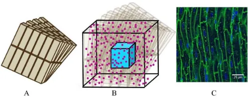
[image:2.612.314.563.56.157.2]A model of a simplified volume of left ventricular myocardium was created as shown in Fig. 1. Cells were modelled as cuboids with a defined length, cross-sectional area and aspect ratio of the cross-section (thickness/width). The model consisted of layers of cells where each layer is parallel to the epicardium and endocardium, that is, transverse angles (those between the circumferential axis and the projection of
Fig. 1. Schematic of model geometry (note model sizes may differ from those in the Figure).(A)Cells are cuboids and are arranged in parallel layers, angled from the adjacent ones.(B)The voxel to be analyzed is the turquoise cube at the center of the total model volume. Molecules (pink) are randomly distributed across the whole model volume.(C) Confo-cal image of cardiomyocytes in long section from Bensleyet al. [18] (CC BY 4.0).
the cell long-axis onto the radial-circumferential plane [19]) were set to 0°. Cells within each layer were parallel to each other. The gaps between cells within and between layers was equal and was chosen to give the desired volume fraction of cells, that is, the proportion of the tissue made up of myocytes. Fig. 1Cshows a confocal image of myocytes where it can be seen that they are regularly packed and similar in size. To aid interpretation of the simulation data, the model is simplified and the cells are modelled as all the same size and evenly packed within each layer.
The helix angle (that between the cell long-axis projected onto a plane parallel to the epicardium, and the radial-circumferential plane [19]) varied linearly across the voxel at a rate based on the ratio between the range of helix angles found across the myocardium and typical left ventricular (LV) wall thickness (see Table I). The LV wall thickness in the literature ranged from 1.73 mm to 2.67 mm [20]–[22], and the total helix angle variation ranged from 130° to 180° [8], [19], [23]. For the comparisons with experimental data, the resultant angle between cells in adjacent planes is 1.0°; it is variable for the sensitivity analysis due to its dependence on the cell size, volume fraction and angle rate.
A single cubic voxel was analyzed. To avoid boundary effects a cube with sides 200 μm larger than the required voxel was modelled. Molecules were randomly distributed, from a uniform density law, across the simulation volume in both the IC and EC space; at every time step each molecule’s displacement along each of the three axes is taken from a normal distribution with a mean of zero and the standard deviation equal to the 1D step length of√2Dδt where D is the diffusivity and t is the timestep. If a molecule reaches any boundaries, it reflects elastically off those boundaries. Colli-sions between molecules are not modelled. Initial experiments showed that a minimum density of 1×10⁸molecules/mm3 and a maximum timestep of 2μs were required for accurate and repeatable results.
The diffusivity was assumed to be isotropic, and to be the same in the IC and EC space. The restrictions to diffusion from surfaces other than the cell membranes were not modelled explicitly, but assumed to be incorporated in the diffusivity, which is lower than the self-diffusivity of water.
TABLE I
MODELPARAMETERS
sensitivity analysis chosen to match the range of values reported in different publications, and the model parameters for the comparison with experimental data in the middle of this range, as listed in Table I.
B. Diffusion Simulations
The total phase shift,ϕ, for each molecule was a function of the gradient strength that it experienced over every timestep j , dependent on its location at that time, and was calculated as [37]:
ϕ =
N
j=0 ϕj =
N
j=0
γG(tj),r(tj)t (1)
where N is the total number of timesteps, G(tj)is the magnetic field gradient at timestep j , r(tj)is the molecule position at timestep j , t is the timestep, and γ is the gyromagnetic ratio (267.5rad/μs/T for protons).
The MRI sequence modelled was the standard Stejskal-Tanner sequence [38], with rectangular diffusion gradient pulses assumed. The gradient strength at the location of the molecule at each timestep was summed for the duration of the two pulses of spatially-varying gradients, with the second pulse given a negative sign.
Only those molecules which finished in the central voxel were used to calculate the MRI signal. The MRI signal, S/S0, for M molecules for each gradient direction is:
S S0 =
1 M
M
i=1
cos(ϕi) (2)
C. Calculation of MRI Measurements
In DT imaging, the b-value is the diffusion weighting which combines the properties of the applied gradient pulse
into a single factor. In the idealized free diffusion state for rectangular pulses, this is given by:
b=(Gγ δ)2
−δ 3
(3)
where G is the magnetic field gradient strength, δ is the diffusion gradient pulse duration, and is the time between gradient pulse onsets. For experimental data cross terms between the diffusion and imaging gradients, and nonzero ramp times also contribute to the b-value. In this work, we achieve a range of b-values by varying both the gradient strength and pulse timing parameters.
The diffusion tensor was calculated for each voxel using linear fitting, and from this the commonly used measures FA and MD were calculated as [6]:
M D= λ1+λ2+λ3
3 (4)
F A=
3 2
λ1− ¯λ
2
+ λ2− ¯λ 2
+ λ3− ¯λ 2
λ2 1+λ
2 2+λ
2 3
(5)
where λn is the nth eigenvalue and λ¯ is the mean of the eigenvalues.
D. Simulation of Noise
MRI acquisition noise was added to the simulated data using a Rician noise model [39]:
S =S∗+N1+i N2 (6)
TABLE II
DTI SEQUENCEPARAMETERS
gain was optimized for each diffusion-weighting [40]. For the simulations, noise was added to the noise-free signal for 100 repetitions, which was shown in initial experiments to give stable results. The DT was then calculated for each repetition, and the mean and standard deviation over all the repetitions is reported.
E. Experimental Data
Hearts from five healthy Sprague-Dawley rats were isolated, fixed with isosmotic Karnovsky’s fixative with 2 mM Gd (Prohance, Bracco, MN, USA), rinsed and embedded in 1% agarose gel comprising PBS and 2 mM Gd [41]. Experimental investigations conformed to the UK Home Office guidance on the Operations of Animals (Scientific Procedures) Act 1986 and were approved by the University of Oxford’s ethical review board.
Diffusion spectrum imaging (DSI) data were acquired on a 9.4T horizontal bore MRI scanner (Agilent, CA, USA) with shielded gradients (maximum gradient strength=1T/m,), rise time =130μs, and a transmit/receive quadrature-driven birdcage coil (inner diameter = 20 mm; Rapid Biomedical, Rimpar, Germany). We used a 3D fast spin echo sequence: TR/TE = 250/15 ms, echo train length = 8, echo spac-ing=4 ms, FOV=20×16×16 mm, matrix=100×80×80, isotropic resolution=200μm, diffusion duration (δ)=5 ms, diffusion time ()= 9ms, number of non-DW images = 4, number of DW directions/b-values = 257, b-value (max) = 10,000 s/mm2, acquisition time =14:30 h.
For each b-value, the MRI signals for each voxel were calculated and normalized to the S0 signal. The MRI signals were analyzed in two ways. Firstly, the mean, median and interquartile ranges of these MRI signals were calculated across all the voxels and gradient directions for each of the b-values.
Secondly, the MRI signals were analyzed in the directions of the DT’s eigenvectors. Since the DSI gradients are in a grid layout aligned with the co-ordinate system axes, there are five b-values acquisitions along each of the co-ordinate axes. The DT was calculated for all b-values up to 3000 s/mm2. All voxels where the eigenvectors of the DT aligned to within 8° of the co-ordinate system axes were identified, and the largest
continuous volume of these voxels was taken to avoid noisy voxels. The MRI signals for the gradient directions along the co-ordinate system axes were averaged over all those voxels for each b-value.
In addition, the data were divided up into sets by b-value, where the b-value has a range of no more than 400 s/mm2, and DT analysis carried out. A 3D region of interest (ROI) was manually defined within the left ventricle, with reference to high-resolution anatomical images. Care was taken to avoid regions containing buffer, gel or residual blood, thus avoiding the unwanted influence of these non-representative areas. The ROIs had a volume of at least 1.6 mm3(200 voxels).
A second 3D echo planar DTI dataset was acquired with four different diffusion times and five b-values to investigate the effect of different diffusion times: TR/TE = 250/10 ms, echo train length = 16, FOV = 20 × 16 × 16 mm, matrix = 40× 32× 32, isotropic resolution = 500 μm, δ = 2.5 ms, = 10, 20, 30 and 40 ms, number of non-DW images =5, number of DW directions =6, b-value = 400, 800, 1600, 3200 and 6400 s/mm2, acquisition time = 1:20 h. For each combination of diffusion time and b-value, the MRI signals were analyzed over all voxels and gradient directions and the DT analysis was carried out. Due to the poorer spatial resolution of the second dataset, the heart was segmented from the background by thresholding on the b0 image and the whole heart was analyzed.
F. Analysis of Simulation MRI Signal
The settings for the simulations were chosen to match the settings for the experimental data, and are listed in Table II. The MRI signals from the experimental data were analyzed over all of the gradient directions and all of the voxels, each of which will have had a different microstructure and orientation of that microstructure compared to the gradient directions. In the simulation, there was only a single voxel. To mimic the experimental variation of gradient directions in relation to the microstructure, the number of gradient directions was set to 100.
Fig. 2. Eigenvalues as b-value is changed by gradient strength from the 5 hearts in the experimental data. Pink line indicates the average of all 5 hearts. Data are the mean±standard deviation over all voxels.
identified (the difference between eigenvector and gradient direction was less than 8°), and the MRI signals in these directions were compared to the experimental data.
G. Membrane Permeability
The cell membranes in the studies up to here are assumed to be impermeable. However, cell membranes are not com-pletely impermeable to water molecules and the inclusion of permeability in modelling has been shown to affect the results, especially the FA [14], [42]. To test whether permeable membranes affect the results in this model, we performed a series of experiments with the membrane permeability set to 15 μm/s [43]. All other parameters were as for the effect of gradient strength in Table II.
H. Sensitivity Analysis
For the sensitivity analysis, the modified Morris method [44] was used. This is a simple and economic type of sensitivity analysis, which screens the input factors to determine which are the most important, and was therefore chosen for this study. It takes interactions of factors into account and is model independent. It assumes no stochasticity in the model, which is not strictly true for this model; however, the variation due to stochasticity is much smaller than that due to the changes in the input factors. It produces two sensitivity measures for each input factor:μ∗is the estimated mean of the elementary effects and estimates the overall effect of the factor on the output, andσ is the standard deviation of the elementary effects and estimates non-linear effects and interactions with other fac-tors. The parameters were varied between the maximum and minimum values shown in Table I.
I. Software
The model was created in Smoldyn [45]. Custom-written MATLAB (MathWorks, Massachusetts, USA) code was used to calculate the diffusion MRI signals, and to carry out the dif-fusion tensor analysis. The sensitivity analysis was performed using the modified Morris method software implemented in MATLAB and provided by Campolongo et al. [44].
III. RESULTS
[image:5.612.315.562.59.193.2]The eigenvalues of the experimental data are shown in Fig. 2. Visual inspection shows consistent results across the five hearts; the average of them was therefore used when comparing with the simulated data.
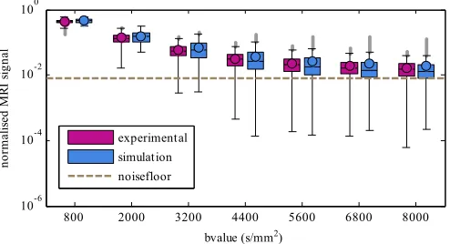
Fig. 3. Effect of b-value changed by gradient strength on MRI signals. Boxes are inter-quartile ranges with the median as a horizontal line and the circle indicating the mean; whiskers are 1.5 times the interquartile range, and outliers are beyond that. Dashed line indicates the approximate noise floor.
Fig. 4. Effect of diffusion time (Δ) on MRI signals for experimental and simulated data for b-values of 400 and 1600s/ mm2. Boxes are inter-quartile ranges with the median as a horizontal line and the circle indicating the mean; whiskers are 1.5 times the interquartile range, and outliers are beyond that.
The simulation voxel sizes were chosen to match the differ-ent voxel sizes in the experimdiffer-ental data; however, the voxel size makes only a small difference to the simulated results.
A. MRI Signals
Fig. 3shows the effect of changing the b-value by gradient strength on the MRI signals for the simulated and experimental data. The difference between the experimental and simulated means and medians is no more than 17% across the whole range of b-values, and the MRI signal attenuation increases for both as the b-value increases. The experimental data has a smaller inter-quartile range than the simulated data. The simulated data has fewer very small values than the experimental data, and its mean is larger than the median, especially at higher b-values.
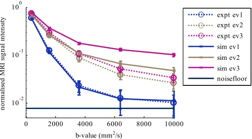
[image:5.612.313.563.265.399.2]Fig. 5. Effect of b-value changed by gradient strength on MRI signals in the directions of the eigenvectors (ev) of the DT for experimental (dotted line) and simulated (solid line) data. Solid dark line indicates the approximate noise floor. Colors are used to differentiate primary (blue), secondary (beige) and tertiary (pink) eigenvector directions.
Fig. 6. Effect of b-value changed by gradient strength on eigenvalues (λ) for the simulated (solid lines) and experimental (dotted lines) data. Data points are mean values over all voxels and all hearts (expt), and all repetitions (sim); error bars are±1 standard deviation. Colors are used to differentiate primary (blue), secondary (beige) and tertiary (pink) eigenvalues.
median and inter-quartile range of the MRI signals are very close to the experimental data. The mean, median and inter-quartile range increases slightly for the experimental data as the diffusion time increases; the simulated data also increase but more quickly leading to a maximum difference in the mean values of 43%.
Fig. 5 shows the effect of changing the b-value by gra-dient strength on the MRI signals in the directions of the eigenvectors of the DT for the simulated and experimental data. The simulated signals in the direction of the primary eigenvector are no more than 10% different compared with the experimental data. The simulated signals in the directions of the secondary and tertiary eigenvectors are higher than the experimental data, but decrease in a similar manner with b-value.
B. Diffusion Tensor and Derivatives
Fig. 6shows the comparison of the experimental and sim-ulated results for the effect of b-value by gradient strength on the eigenvalues of the diffusion tensor. Both the experimental and simulated eigenvalues decrease with increasing b-value.
[image:6.612.316.562.61.185.2] [image:6.612.315.560.251.377.2]Fig. 7. Effect of b-value changed by gradient strength on MD (left) and FA (right) for the simulated (solid lines) and experimental (dotted lines) results. Data points are mean values over all voxels and all hearts (expt), and all repetitions (sim); error bars are±1 standard deviation.
Fig. 8. Effect of diffusion time (Δ) on eigenvalues for simulated (solid lines) and experimental (dotted lines) data for b=1600 s/ mm2. Data points are mean values over all voxels and all hearts (expt), and all repetitions (sim); error bars are±1 standard deviation.
The primary eigenvalue is higher for the noisy simulated data than the experimental data, while the secondary and tertiary eigenvalues are lower than the experimental data, leading to a good estimation of the MD in the simulated data, and an overestimation of the FA, as seen inFig. 7.
Fig. 8shows the effect of the diffusion time on the eigenval-ues of the diffusion tensor for the simulated and experimental data for a b-value of 1600 s/mm2. All of the experimental and simulated eigenvalues decrease as the diffusion time increases. The simulated primary eigenvalue matches the experimental data well. The secondary and tertiary eigenvalues are lower than the experimental ones, especially at longer diffusion times.
Fig. 9 shows the effect of permeable membranes on the eigenvalues, MD and FA. The simulation with permeable membranes results in a slightly lower FA. Figure 10shows the effect of permeable membranes on the MRI signals. As the diffusion time is increased, the permeable membranes lead to lower MRI signals than impermeable membranes.
C. Sensitivity Analysis
[image:6.612.53.297.262.405.2]Fig. 9. Effect of permeability on eigenvalues, MD and FA. b-value is changed by gradient strength. Values are mean ±1 standard deviation.
Fig. 10. Effect of permeability on MRI signals for experimental and simulated data for a b-value of 1600 s/ mm2 as diffusion time (Δ) is changed. Boxes are inter-quartile ranges with the median as a horizontal line and the circle indicating the mean; whiskers are 1.5 times the interquartile range, and outliers are beyond that.
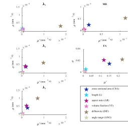
little interaction with the other factors. For the secondary and tertiary eigenvalues, the FA and the MD, the cross-sectional area is the next most important factor. The aspect ratio is important for the secondary and tertiary eigenvalues and the FA. The length, angle rate and volume fraction have only very small effects on all the outcomes.
D. Computing Time
[image:7.612.52.299.360.492.2]For an isotropic voxel of 200μm, with a 200μm border (i.e. a volume of 400μm×400μm×400μm), the total com-putational time on a desktop PC for a diffusion time of 44 ms is 300 h. Simulation of the diffusion in Smoldyn takes a total of 180 h, in 50 separate simulations of 3.5 h. Converting the text output files from Smoldyn into MATLAB format takes a
Fig. 11. Sensitivity analysis results for primary, secondary and tertiary eigenvalues (left, top to bottom), MD (right, top) and FA (right, middle). μ∗. estimates the overall effect of the factor;μ∗estimates non-linear effects and interactions with other factors.
total of 100 hours (7 minutes per file for a total of 800 files). Calculation of the MRI signal in MATLAB takes 20 h.
IV. DISCUSSION
The first aim of this study was to demonstrate a modelling methodology for the acquisition of diffusion weighted images of myocardial tissue, and to assess its results compared with experimental data. The model reproduces the MRI signals well compared with the experimental data. The DT and its derivatives also correspond well with the experimental data.
The simulated MRI signal in the direction of the primary eigenvector is very close to the experimental data, while for the secondary and tertiary directions the simulated signal is less attenuated than the experimental data. The eigenvalues of the DT show similar results to the MRI signals. The noisy primary eigenvector is similar to the data, while the simulated secondary and tertiary eigenvalues are lower than the exper-imental ones. These eigenvalues lead to a similar MD in the noisy simulated and experimental data, while the FA is higher in the simulations than the experiments at lower b-values and then decreases more rapidly than the experimental FA.
experiment. This leads to greater differences in the eigenvalues of the DT, and therefore a higher FA in the simulated data.
The MRI signal attenuation decreases with increasing dif-fusion time as a result of increased interactions with cell restrictions. This effect is more pronounced in simulation than in the experimental data (the mean MRI signal in simula-tions / experiments were 55% / 19% higher at = 40 ms compared with = 10 ms). Incorporation of membrane permeability in the simulations reduced the signal differences from 55% to 48%. In addition to permeability, the differences in diffusion time dependence between the simulated and experimental data are likely to arise from the highly ordered arrangement of simulated cells.
The addition of permeable membranes had only a small effect on the dMRI results. This is in agreement with Wang et al. [14] for physiologically realistic values of per-meability, but Hall and Clark [42] found much greater effects from the inclusion of permeability. Our experiments up to this point have only included a single value of permeability, and have not explored the relationships between permeability and volume fraction. Further exploration of these aspects might help clarify differences between studies.
Even though the model does not explicitly include sheetlets, the secondary and tertiary eigenvalues are clearly distinct in the simulated data, as seen inFigs. 6and8. This difference in eigenvalues is likely to derive from two factors: the difference in the width and depth of the cross-section of the cells, and the dispersion of cell orientations within a voxel. It may therefore be that some of the difference in eigenvalues in the experiments derives from the shapes of the cells in addition to the sheetlets.
The second aim of this study was to determine which of six factors concerning simplified cell shape and tissue structure have the greatest influence on cardiac DTI results. This is important for two reasons: firstly, as there is a large range of values in the literature for each parameter, it allows us to understand for which parameters the choice of value is critical to the model output. Secondly, as these parameters may change with pathology, it helps understand the effect of pathological changes in microstructure in diffusion MRI signals, and design MRI sequences that respond to changes in particular parameters.
The diffusivity was by far the most important factor, especially for the primary eigenvalue and the MD. As the diffusivity increases, the mean squared displacement of water in a given time increases thus increasing the eigenvalues. In free space, this would be a linear relationship, but in the restricted case, as the step distance increases, the likelihood of interaction with a surface (cell membrane) increases, resulting in reduced phase dispersion and apparent diffusivity. As car-diomyocytes are long narrow structures, these interactions tend to preferentially decrease the secondary and tertiary eigen-values, compared to the primary eigeneigen-values, in a nonlinear manner. There is a wide range of values available for the diffu-sivity in the literature since the diffudiffu-sivity is dependent on the measurement technique and the temperature: this uncertainty is a significant limitation to the model. However, since theσ is low, there is little non-linearity or interaction with other factors
and therefore the relative results of simulations should not be affected significantly by the diffusivity. Diffusivity is assumed to be a single value, which is the same in all directions within the cell and outside it. IC structures and the EC matrix will affect the rate of diffusion. This may not be the same intra-and extra- cellularly, as suggested by Garrido et al. [34], nor the same in each direction in the cell. Disease may affect the IC and EC environments and thus the diffusivity. Experimental investigation of these effects, especially in pathology, would enhance the model and the understanding of DTI in disease. A further implication of these findings is that dMRI analysis models which assume a fixed diffusivity value may be sensitive to the value selected which could affect the model fitting.
The cross-sectional area has an effect on the secondary and tertiary eigenvalues, the MD and the FA, although its effect is much smaller than the diffusivity. A smaller cross-sectional area leads to an increase in molecule-surface interactions which will decrease the mean squared displacement within the cross-sectional plane and therefore the secondary and tertiary eigenvalues. The aspect ratio is as important as the CSA for the secondary and tertiary eigenvalues, and the FA. A smaller aspect ratio (greater difference between thickness and width) will cause a greater difference in the diffusion in the direction of the thickness compared with the width and hence a larger secondary and smaller tertiary eigenvalue for the same CSA, and a higher FA.
The length, volume fraction and rate of helix angle change have negligible effects on all three eigenvalues. The VF changes the size of the gaps between cells in the simulation but even though this makes the EC space more restrictive than the IC space, since the proportion of EC space is small, changes in the VF do not significantly affect the DT. Since the cells are much longer than they are wide or thick, molecule-surface interactions with the ends of the cells are infrequent compared with those with the sides and hence the length does not have a large effect on the results. The ANG is small over a single voxel and therefore has little effect.
the rate of angle change (i.e. the angle between cell layers), which is the parameter that would be affected by such noise. The model does not yet include myocardial disarray, which can be found in disease. The introduction of myocardial disarray into the model would assist in the understanding of the effect of disease on DTI results. At this stage we model only a single voxel and do not therefore generate MRI images for comparison with experimental data. Future work could include simulations of multiple voxels or even a whole heart model, following on from Wang et al. [16]. At that stage, analysis of helix angles would also become interesting.
The sensitivity analysis results are interesting when consid-ered in the context of pathological changes, which include disarray, fibrosis, cell hypertrophy and IC changes [46]. In hypertrophy, the CSA of cells increases and this may therefore be detected through changes in MD or FA. Fibrosis is characterized by a proliferation of fibroblasts and the formation of connective tissue, and leads to a smaller vol-ume fraction of myocytes. However, the current model only represents myocytes, and thus does not yet allow an accurate representation of fibrosis. It is possible to introduce these pathological changes into this model and we hope therefore to use the model to further understanding of the relationship between disease and the MRI signal that is produced.
The noise model is of MRI acquisition noise; biological variation is not included in the model. The sensitivity analysis suggests that variation in the cross-sectional area and aspect ratio of the cells would have an effect on the results, whereas the length, helix angles and volume fraction would make a comparably small difference. Future work should therefore focus on introducing variability in those parameters likely to make a significant difference on the results.
The current model is computationally expensive and this is a limitation to further work with the model. There are several ways in which this could be improved. Reducing the boundary around the voxel would speed up the two most intensive parts of the process: the generation of the data in Smoldyn and the conversion of the data into MATLAB. The implementation of the pipeline in a single framework, in which the particle diffusion results could be directly read by the MRI signal generation software without writing and reading them from the hard drive would also represent a significant reduction in computational time. Combining analytical signals for appro-priate structures with MC simulation would be another way to reduce the computation time.
We acknowledge that modelling high b-value data with the DT model violates the model’s assumption that the O(b2) term is negligible relative to noise. However, we found that this model is nevertheless useful in comparing the experimen-tal and simulated MR signals. While non-Gaussian models such as the diffusion kurtosis [47], bi-exponential [48] or anomalous diffusion [49] models may be more appropriate for the comparison of high b-value data, the application of such models is outside the scope of this work. In addition, we note that in order to minimise TE and achieve sufficient SNR experimentally at the specified b-values and spatial resolution, δ was necessarily non-negligible. However, simulations by Balinov et al. with δ ∼ show that the accuracy of both
the short gradient pulse limit and Gaussian phase distribu-tion estimates of the diffusion signal improves with larger sphere radius or separation between parallel planes [37]. We considered the finite δ to be reasonable given the relatively large∼14μm diameter of cardiomyocytes in our simulations. We have demonstrated a modelling method of DTI in the heart which provides an excellent match of MRI signals to experimental data, and can therefore be considered to be a useful tool in investigating cardiac diffusion MRI. Further validation against data where the exact structure is known could be valuable, for example for cardiac tissue where his-tology and DTI data are both available, or against a phantom model such as that used by Teh et al. [50]. While DTI can be a sensitive marker of pathological changes, it is not particularly specific. By better understanding the dominant tissue properties that affect the DTI results, we can prioritize development of models and acquisition strategies that enable estimation of such properties from DTI data. Improving the specificity of DTI measurements could augment the potential of DTI as an early biomarker of pathology in the heart, and our ability to distinguish between subtler forms of disease, such as different forms of disarray. Further work will introduce myocardial disarray into the model and investigate other output measures.
REFERENCES
[1] D. Streeter, H. M. Spotnitz, D. P. Patel, J. Ross, and E. H. Sonnenblick, “Fiber orientation in the canine left ventricle during diastole and systole,”
Circuit Res., vol. 24, no. 3, pp. 339–347, 1969.
[2] I. J. LeGrice, B. H. Smaill, L. Z. Chai, S. G. Edgar, J. B. Gavin, and P. J. Hunter, “Laminar structure of the heart: Ventricular myocyte arrangement and connective tissue architecture in the dog,” Amer. J.
Physiol.-Heart Physiol., vol. 269, no. 2, pp. H571–H582, 1995.
[3] T. Edvardsen et al, “Regional diastolic dysfunction in individuals with left ventricular hypertrophy measured by tagged magnetic resonance imaging—the multi-ethnic study of atherosclerosis (MESA),” Amer.
Heart J., vol. 151, no. 1, pp. 109–114, 2006.
[4] M. Takeuchi et al., “Reduced and delayed untwisting of the left ventricle in patients with hypertension and left ventricular hypertrophy: A study using two-dimensional speckle tracking imaging,” Eur. Heart J., vol. 28, no. 22, pp. 2756–2762, 2007.
[5] C. G. Brilla, J. S. Janicki, and K. T. Weber, “Impaired diastolic function and coronary reserve in genetic hypertension. Role of interstitial fibrosis and medial thickening of intramyocardial coronary arteries,” Circuit
Res., vol. 69, no. 1, pp. 15–107, 1991.
[6] P. J. Basser and C. Pierpaoli, “Microstructural and physiological features of tissues elucidated by quantitative-diffusion-tensor MRI,” J. Mag.
Reson., vol. 213, no. 2, pp. 560–570, 1996.
[7] J. Chen et al., “Remodeling of cardiac fiber structure after infarction in rats quantified with diffusion tensor MRI,” Amer. J. Physiol.-Heart
Circulat. Physiol., vol. 285, no. 3, pp. H946–H954, 2003.
[8] P. F. Ferreira et al., “In vivo cardiovascular magnetic resonance diffusion tensor imaging shows evidence of abnormal myocardial laminar orienta-tions and mobility in hypertrophic cardiomyopathy,” J. Cardiovascular
Mag. Reson., vol. 16, p. 87, Nov. 2014.
[9] E. Tunnicliffe et al., “Intercentre reproducibility of cardiac apparent diffusion coefficient and fractional anisotropy in healthy volunteers,”
J. Cardiovascular Mag. Reson., vol. 16, no. 1, p. 31, 2014.
[10] M. G. Hall and D. C. Alexander, “Convergence and parameter choice for Monte-Carlo simulations of diffusion MRI,” IEEE Trans. Med. Imag., vol. 28, no. 9, pp. 1354–1364, Sep. 2009.
[11] A. Duh, A. Mohoriˇc, and J. Stepišnik, “Computer simulation of the spin-echo spatial distribution in the case of restricted self-diffusion,” J. Mag.
Reson., vol. 148, no. 2, pp. 257–266, 2001.
[13] E. Fieremans et al., “Simulation and experimental verification of the diffusion in an anisotropic fiber phantom,” J. Mag. Reson., vol. 190, no. 2, pp. 189–199, 2008.
[14] L. Wang, Y.-M. Zhu, H. Li, W. Liu, and I. E. Magnin, “Simulation of diffusion anisotropy in DTI for virtual cardiac fiber structure,” in Lecture
Notes in Computer Science, vol. 6666. Berlin, Germany: Springer, 2011,
pp. 95–104.
[15] L. Wang, Y. Zhu, H. Li, W. Liu, and I. E. Magnin, “Multiscale modeling and simulation of the cardiac fiber architecture for DMRI,” IEEE Trans.
Biomed. Eng., vol. 59, no. 1, pp. 16–19, Jan. 2012.
[16] L. H. Wang, Y.-M. Zhu, F. Yang, W.-Y. Liu, and I. E. Magnin, “Simulation of dynamic DTI of 3D cardiac fiber structures,” in
Proc. IEEE 11th Int. Symp. Biomed. Imag. (ISBI), May 2014,
pp. 714–717.
[17] J. Bates, I. Teh, P. Kohl, J. E. Schneider, and V. Grau, “Sensitivity analysis of diffusion tensor MRI in simulated rat myocardium,” Lecture
Notes in Computer Science, vol. 9126. Cham: Springer, 2015, pp. 120–
128.
[18] J. G. Bensley, R. de Matteo, R. Harding, and M. J. Black, “Three-dimensional direct measurement of cardiomyocyte volume, nuclearity, and ploidy in thick histological sections,” Sci. Rep., vol. 6, Apr. 2016, Art. no. 23756.
[19] P. W. Hales, J. E. Schneider, R. A. Burton, B. J. Wright, C. Bollensdorff, and P. Kohl, “Histo-anatomical structure of the living isolated rat heart in two contraction states assessed by diffusion tensor MRI,”
Prog. Biophys. Molecular Biol., vol. 110, nos. 2–3, pp. 319–330,
Oct. 2012.
[20] W. Kromen et al., “Correlation of left ventricular wall thickness, heart mass, serological parameters and late gadolinium enhancement in cardiovascular magnetic resonance imaging of myocardial inflam-mation in an experimental animal model of autoimmune myocardi-tis,” Int. J. Cardiovascular Imag., vol. 28, no. 8, pp. 1983–1997, 2012.
[21] J. Chen et al., “Regional ventricular wall thickening reflects changes in cardiac fiber and sheet structure during contraction: Quantification with diffusion tensor MRI,” Amer. J. Physiol.-Heart Circul. Physiol., vol. 289, no. 5, pp. H1898–H1907, 2005.
[22] R. M. McAdams, R. J. McPherson, N. M. Dabestani, C. A. Gleason, and S. E. Juul, “Left ventricular hypertrophy is prevalent in Sprague-Dawley rats,” Comput. Med., vol. 60, no. 5, pp. 357–363, 2010.
[23] D. Benoist et al., “Cardiac arrhythmia mechanisms in rats with heart failure induced by pulmonary hypertension,” Amer. J. Physiol.-Heart
Circul. Physiol., vol. 302, no. 11, pp. H2381–H2395, 2012.
[24] A. M. Yeveset al, “Physiological cardiac hypertrophy: Critical role of AKT in the prevention of NHE-1 hyperactivity,” J. Molecular Cellular
Cardiol., vol. 76, pp. 186–195, Nov. 2014.
[25] Y.-F. Chen et al., “Post-myocardial infarction left ventricular myocyte remodeling: Are there gender differences in rats?” Cardiovascular
Pathol., vol. 20, no. 5, pp. e189–e195, 2011.
[26] A. M. Gerdes, J. A. Moore, J. M. Hines, P. A. Kirkland, and S. P. Bishop, “Regional differences in myocyte size in normal rat heart,” Anatomical
Rec., vol. 215, no. 4, pp. 420–426, 1986.
[27] S. E. Campbell, A. M. Gerdes, and T. D. Smith, “Comparison of regional differences in cardiac myocyte dimensions in rats, hamsters, and guinea pigs,” Anatomical Rec., vol. 219, no. 1, pp. 53–59, 1987.
[28] S. E. Campbell, K. Rakusan, and A. M. Gerdes, “Change in cardiac myocyte size distribution in aortic-constricted neonatal rats,” Basic Res.
Cardiol., vol. 84, no. 3, pp. 247–258, 1989.
[29] S. P. Bishop and J. L. Drummond, “Surface morphology and cell size measurement of isolated rat cardiac myocytes,” J. Molecular Cellular
Cardiol., vol. 11, no. 5, pp. 423–433, 1979.
[30] H. Satoh, L. M. Delbridge, L. A. Blatter, and D. M. Bers, “Surface: Vol-ume relationship in cardiac myocytes studied with confocal microscopy and membrane capacitance measurements: Species-dependence and developmental effects,” Biophys. J., vol. 70, no. 3, pp. 1494–1504, 1996.
[31] A. M. Gerdes, T. Onodera, X. Wang, and S. A. McCune, “Myocyte remodeling during the progression to failure in rats with hypertension,”
Hypertension, vol. 28, no. 4, pp. 609–614, 1996.
[32] P. Anversa, R. Ricci, and G. Olivetti, “Quantitative structural analysis of the myocardium during physiologic growth and induced cardiac hypertrophy: A review,” J. Amer. College Cardiol., vol. 7, no. 5, pp. 1140–1149, 1986.
[33] M. A. Rossi and L. C. Peres, “Effect of captopril on the prevention and regression of myocardial cell hypertrophy and interstitial fibrosis in pressure overload cardiac hypertrophy,” Amer. Heart J., vol. 124, no. 3, pp. 700–709, 1992.
[34] L. Garrido, V. J. Wedeen, K. K. Kwong, U. M. Spencer, and H. L. Kantor, “Anisotropy of water diffusion in the myocardium of the rat,” Circul. Res., vol. 74, no. 5, pp. 789–793, 1994.
[35] R. E. Safford, E. A. Bassingthwaighte, and J. B. Bassingthwaighte, “Diffusion of water in cat ventricular myocardium,” J. Generat. Physiol., vol. 72, no. 4, pp. 513–538, 1978.
[36] J. G. Seland et al., “Determination of water compartments in rat my-ocardium using combined D T1and T1-T2experiments,” Mag. Reson. Imag., vol. 23, no. 2, pp. 353–354, 2005.
[37] B. Balinov, B. Jonsson, P. Linse, and O. Soderman, “The NMR self-diffusion method applied to restricted self-diffusion. Simulation of echo attenuation from molecules in spheres and between planes,” J. Mag.
Reson. Ser. A, vol. 104, no. 1, pp. 17–25, 1993.
[38] E. O. Stejskal and J. E. Tanner, “Spin diffusion measurements: Spin echoes in the presence of a time-dependent field gradient,” J. Chem.
Phys., vol. 42, no. 1, pp. 288–292, 1965.
[39] H. Gudbjartsson and S. Patz, “The Rician distribution of noisy MRI data,” Mag. Reson. Med., vol. 34, no. 6, pp. 910–914, 1995.
[40] I. Teh et al., “Resolving fine cardiac structures in rats with high-resolution diffusion tensor imaging,” Sci. Rep., vol. 6, Jul. 2016, Art. no. 30573.
[41] D. McClymont, I. Teh, H. J. Whittington, V. Grau, and J. E. Schneider, “Prospective acceleration of diffusion tensor imaging with compressed sensing using adaptive dictionaries,” Mag. Reson. Med., vol. 76, no. 1, pp. 248–258, 2016, doi: 10.1002/mrm.25876.
[42] M. G. Hall and C. A. Clark, “Diffusion in hierarchical systems: A simulation study in models of healthy and diseased muscle tissue,”
Magn. Res. Med., to be published, doi: 10.1002/mrm.26469.
[43] T. Ogura, S. Imanishi, and T. Shibamoto, “Osmometric and water-transporting properties of guinea pig cardiac myocytes,” Jpn. J. Physiol., vol. 52, no. 4, pp. 333–342, 2002.
[44] F. Campolongo, J. Cariboni, and A. Saltelli, “An effective screening design for sensitivity analysis of large models,” Environ. Modell. Softw., vol. 22, no. 10, pp. 1509–1518, 2007.
[45] S. S. Andrews, N. J. Addy, R. Brent, and A. P. Arkin, “Detailed simulations of cell biology with Smoldyn 2.1,” PLOS Comput. Biol., vol. 6, no. 3, p. e1000705, 2010.
[46] S. Noda, “Histopathology of endomyocardial biopsies from patients with idiopathic cardiomyopathy: Quantitative evaluation based on mul-tivariate statistical analysis,” Circulation J., Official J. Jpn. Circulation
Society, vol. 44, no. 2, pp. 95–116, 1980.
[47] J. H. Jensen, J. A. Helpern, A. Ramani, H. Lu, and K. Kaczynski, “Diffusional kurtosis imaging: The quantification of non-Gaussian water diffusion by means of magnetic resonance imaging,” Mag. Reson. Med., vol. 53, no. 6, pp. 1432–1440, 2005.
[48] T. Niendorf, R. M. Dijkhuizen, D. G. Norris, M. van Lookeren Campagne, and K. Nicolay, “Biexponential diffusion attenuation in var-ious states of brain tissue: Implications for diffusion-weighted imaging,”
Mag. Reson. Med., vol. 36, no. 6, pp. 847–857, 1996.
[49] A. Bueno-Orovio, I. Teh, J. E. Schneider, K. Burrage, and V. Grau, “Anomalous diffusion in cardiac tissue as an index of myocardial microstructure,” IEEE Trans. Med. Imag., vol. 35, no. 9, pp. 2200–2207, Sep. 2016.