Nature or nurture?: testing the correlation between stress tolerance and genotype in the coral Acropora millepora on the Great Barrier Reef

Full text

(1)ResearchOnline@JCU. This file is part of the following reference:. Jin, Young Koo (2015) Nature or nurture? Testing the correlation between stress tolerance and genotype in the coral Acropora millepora on the Great Barrier Reef. PhD thesis, James Cook University.. Access to this file is available from:. http://researchonline.jcu.edu.au/46290/ The author has certified to JCU that they have made a reasonable effort to gain permission and acknowledge the owner of any third party copyright material included in this document. If you believe that this is not the case, please contact [email protected] and quote http://researchonline.jcu.edu.au/46290/.

(2) ii. Nature or nurture? Testing the correlation between stress tolerance and genotype in the coral Acropora millepora on the Great Barrier Reef. Thesis submitted by Young Koo Jin July 2015. For the degree of Doctor of Philosophy in the College of Marine and Environmental Sciences James Cook University.

(3) ii. Acknowledgements I am gratefully indebted to my supervisors, Bette Willis, Madeleine van Oppen and Petra Lundgren for giving me the opportunity to explore a field of intriguing marine life, corals, and accomplish the PhD. I would like to thank you for your patience, words of encouragement and wise guidance which helped me push through a difficult time in my life. Your advice on my research has been invaluable for allowing me to grow as a scientist. I would also like to express thanks to researchers at AIMS, especially Lesa Peplow for her help with technical assistance to take my first steps in a lab. Special thanks to Stuart Kininmonth for helping me with Bayesian statistics. He patiently guided me, who had no experience and knowledge about Bayesian statistics and software. Additionally, he provided extremely generous support to greatly improve Chapter 5 with his competent advice. I would like to thank my friends in Townsville, Kero, Aomi, Mona, Jeroen and all the other people for making my time in Townsville special. Finally, my sincere thanks to my daughter, Sana. Despite the hard time we have been going through, she gave me smiles and loved me just as she did before. This gave me strength to continue and finish my thesis..

(4) ii. Statement on the contribution of others The research within this thesis was supported by the Australian Institute of Marine Science (AIMS), funding provided through the Australian Research Council (ARC) Centre of Excellence for Coral Reef Studies, and a James Cook University (JCU) Graduate Research Scheme grant. A supervisory team consisting of Professor Bette Willis (JCU), Dr Madeleine van Oppen (AIMS), and Dr Petra Lundgren (AIMS/Monash University) provided intellectual and editorial support throughout the thesis. Dr Stuart Kininmonth (the Stockholm Resilience Centre) provided statistical help with environmental correlation network analysis in Chapter 3 and statistical, intellectual and editorial support for Chapter 5. Lesa Peplow (AIMS) and Roxana Capper (University of Texas) contributed to the development of the curves method and peaks method, respectively in Chapter 2. Lesa Peplow (AIMS), Jason Doyle (AIMS), Andrew Muirhead (AIMS) provided DNA samples for gene by environment association (Chapter 3). Dr Allison Paley (JCU) and Dr Emily Howells (JCU/AIMS/NY U Abu Dhabi) provided DNA samples and bleaching data (Chapter 4). Dr Jean-Baptiste Raina (JCU/AIMS/UT Sydney) and Dr Adrian Lutz (AIMS/JCU) provided samples and phenotypic data from their heat stress experiment (Chapter 4).

(5) i Abstract Corals are known to have both high phenotypic plasticity and significant capacity for acclimatisation, either through physiological, biochemical and behavioural responses to environmental stochasticity, or through contributions of symbiotic Symbiodinium to the physiological tolerance of the coral holobiont. Local adaptation is suggested by the fact that populations along environmental gradients maintain differences in environmental tolerance after acclimatisation to the same condition, as well as by the existence of correlations between the genetic diversity of coral hosts and environmental gradients in natural coral populations. However, no study has yet identified genetic markers underlying stress tolerance variation in corals. The research presented here aims to improve knowledge of the adaptive importance of genetic diversity within coral populations by: (1) developing a cost- and time-efficient single nucleotide polymorphism (SNP) genotyping method that accurately estimates allele frequencies from pooled samples (Chapter 2); (2) investigating correlations between allele frequencies at candidate loci and temperature and water quality gradients along the Great Barrier Reef (Chapter 3); (3) validating genotypeenvironment correlations at candidate loci for phenotypes associated with bleaching tolerance in both field and laboratory settings (Chapter 4); and, (4) predicting the spatial distribution of allele frequencies at the anti-oxidant capacity loci identified in Chapter 4 through Bayesian belief network modelling (Chapter 5). SNPs are the most common type of genetic variation and are present at both functional and neutral loci, making them ideal markers to study adaptive molecular variation. SNP allele frequency distributions can be used to identify coral populations that show signatures of adaptation to local environmental conditions, because the frequency of genetic variants (i.e., alleles) will vary with selection for or against these.

(6) ii mutations and any other linked loci that affect fitness of the organism. Examination of genomic signatures of environmental change at the population level provides information about the resilience of coral populations at broad geographical scales. Genotyping of pooled DNA for estimating allelic proportions provides a time- and costeffective method for large sample sets. In Chapter 2, I introduce two quantitative High Resolution Melting (qHRM) methods for measuring allele frequencies at known SNP loci in pooled DNA samples: the “peaks” method, which can be applied to large numbers of SNPs, and the “curves” method, which is more labour intensive but also more accurate. In Chapter 3, the distributions of SNP allele frequencies at five functional loci were investigated in 25 populations of Acropora millepora along the Great Barrier Reef using the curves genotyping method. Significant correlations between allele frequencies and gradients in both water quality and temperature were detected at two functional loci. In Chapter 4, I validated the two genetic markers as true quantitative trait loci for anti-oxidant capacity in the common coral, A. millepora. Field surveys revealed that colonies carrying G and T alleles, respectively, at the two loci were significantly less affected by two bleaching events. These results were corroborated in an aquariumbased experiment showing constitutively higher anti-oxidant capacity of colonies with these alleles, particularly in the homozygous state. These genetic markers are located on different chromosomes and closely linked to a range of genes involved in bleachingassociated processes, such as thermal, hypoxic and oxidative stress, suggesting they are indicative of tolerance to a multitude of environmental perturbations. Markers such as the ones identified in this study provide an opportunity to use environmental mapping to identify populations that are resistant to a range of environmental stressors. In Chapter 5, a spatial Bayesian belief network (BBN) model.

(7) iii was developed to predict GBR-wide spatial distributions of allele frequencies at the antioxidant capacity locus C29226S281. A combination of long-term environmental monitoring data, allele frequency data, expert input and statistical evaluation was used to build the model, with the goal of refining prior beliefs and examining dependencies among environmental variables that are proxy indicators of selective forces on allele frequencies at locus C29226S281. The model predicts that a high allele frequency is correlated with poor water quality and large fluctuations in sea temperatures. The Bayesian simulation approach demonstrates that the synergism between highly fluctuating sea temperatures and high nitrate concentrations may be the primary driver in selecting alleles at this locus. High temperature fluctuation in isolation does not increase the probability of finding high allele frequencies. Consistent with this, spatial mapping of predicted allele frequencies reveals that increased anti-oxidant capacity alleles are most likely to be concentrated near the mouths of the Burdekin and Fitzroy Rivers, where nutrient levels are chronically high. Coupling GIS and BBN enables visualisation of the model output, specifically qualitative measurements of allele frequencies, enabling non-experts to explore and interpret complex interactions between environmental and genetic factors. This thesis provides compelling evidence that the two loci identified are true QTLs associated with responses to bleaching-associated stressors. Correlations between the spatial distribution of allele frequencies and genotypic variation associated with bleaching tolerance at the loci indicate the existence of adaptive genetic diversity in current coral populations. These findings open up opportunities for novel coral reef management approaches, such as spatial mapping of stress tolerance for use in Marine Protected Area design, the identification of stress tolerant colonies for assisted migration and marker-assisted selective breeding to create more tolerant genotypes for restoration of denuded reefs..

(8) iv. Contents Abstract. i. List of Tables. viii. List of Figures. ix. Chapter 1.0 Background and General Introduction. 1. 1.1 Responses of coral reefs to climate change on the Great Barrier Reef. 1. 1.2 Role of gene flow in adaptation. 5. 1.3 Identification of genetic markers for gene by environment associations. 7. 1.4 Thesis objectives. 9. Chapter 2.0 Quantitative high resolution melting: two methods to determine SNP allele frequencies from pooled samples. 12. 2.1 Introduction. 13. 2.2 Materials and Methods. 16. 2.2.1 Coral collection. 16. 2.2.2 DNA extraction. 17. 2.2.3 Peaks method. 18. 2.2.3.1 Pooling. 19. 2.2.3.2 Internal melting calibrators. 20. 2.2.3.3 Asymmetric template amplification and melt stage. 20. 2.2.3.4 Analysis of denaturation profiles. 21. 2.2.3.5 DNA titrations. 22. 2.2.3.6 Analysis of 384 loci in six individuals. 24. 2.2.3.7 Analysis of 384 loci in 98 individuals collected from two locations. 24. 2.2.3.8 Analysis of genetic subdivision between coral populations. 25. 2.2.4 Curves method. 25. 2.2.4.1 Pooling. 26. 2.2.4.2 Asymmetric template amplification and melt stage. 26. 2.2.4.3 Analysis of denaturation profiles. 26. 2.2.4.4 DNA titrations and method validation. 28. 2.2.4.5 Application to large pools of DNA. 29. 2.2.4.6 qHRM reproducibility. 29.

(9) v 2.3 Results 2.3.1 Peaks method. 30 30. 2.3.1.1 Allele titrations. 30. 2.3.1.2 Analysis of 384 loci in six individuals. 32. 2.3.1.3 Analysis of 384 loci in 98 individuals collected from two locations. 32. 2.3.1.4 Detection of novel alleles. 34. 2.3.2 Curves method. 35. 2.3.2.1 Allele titrations. 36. 2.3.2.2 Application to large pools of DNA. 36. 2.3.2.3 Reproducibility of qHRM. 37. 2.4 Discussion. 38. 2.4.1 Comparisons with other genotyping methods. 38. 2.4.2 Pooled genotyping by HRM and unlabelled probes. 40. 2.4.2.1 Peaks method. 40. 2.4.2.2 Curves method. 41. 2.5 Conclusion. Chapter 3.0 Allele frequency difference along water quality and temperature gradients at SNP loci in panmictic coral populations. 43. 44. 3.1 Introduction. 46. 3.2. Methods and Materials. 48. 3.2.1 Study sites. 48. 3.2.2 Environmental variables. 49. 3.2.3 Target SNPs. 50. 3.2.4 HRM genotyping. 51. 3.2.5 Statistics. 51. 3.2.5.1 Detection of divergent populations. 51. 3.2.5.2 Gene by environment association. 52. 3.2.5.3 Environmental correlation network. 52. 3.2.5.4 Spatial clustering of water quality and temperature factors. 53. 3.2.5.5 Combined effects of NO3 and temperature range. 53. 3.3 Results 3.3.1 Outlier detection. 53 53.

(10) vi 3.3.2 Gene by environment association. 55. 3.3.3 Environmental and biotic correlation network. 56. 3.3.4 Spatial clustering of water quality and temperature factors. 58. 3.3.5 Combined effects of NO3 and temperature range. 58. 3.4 Discussion. 59. 3.4.1 Gene by Environment association. 59. 3.4.2 Detection of outlier populations. 63. 3.5 Conclusion. Chapter 4.0 Genotype-phenotype association: quantitative trait loci for coral antioxidant capacity. 64. 66. 4.1 Introduction. 67. 4.2 Materials and Methods. 70. 4.2.1 Mendelian inheritance. 70. 4.2.2 Natural bleaching experiment. 70. 4.2.3 Heat stress experiment. 73. 4.2.4 SNP genotyping. 74. 4.2.5 Statistics. 75. 4.2.6 Functions of genes in linkage groups. 75. 4.3 Results. 75. 4.3.1 Mendelian inheritance. 75. 4.3.2 Natural bleaching experiment. 76. 4.3.3 Heat stress experiment. 77. 4.3.4 Linkage study. 79. 4.4 Discussion. Chapter 5.0 Predicting the spatial distribution of allele frequencies for a bleaching tolerance gene in Acropora millepora using Bayesian belief network modelling. 80. 86. 5.1 Introduction. 88. 5.2 Methods and Materials. 90. 5.2.1 Genetic and environmental data. 90. 5.2.2 Environmental correlation network. 92. 5.2.3 Bayesian belief network. 94.

(11) vii 5.2.4 Predictability of BBN model. 97. 5.2.5 Sensitivity analysis. 98. 5.2.6 Simulation analysis. 98. 5.2.7 Spatial mapping. 98. 5.3 Results. 99. 5.3.1 Prediction of likelihood of allele frequencies through BBN. 99. 5.3.2 Sensitivity. 102. 5.3.3 Predictability (error rates). 103. 5.4 Discussion. 104. Chapter 6.0 General discussion. 109. 6.1 Major findings of this thesis and their implications. 109. 6.2 Further considerations and recommendations arising from thesis results. 111. 6.3 Future research directions. 114. References. 118. Appendices. 132.

(12) viii. List of Tables Table 2.1. Collection year, sample size, latitudes and longitudes of 28 populations Table 2.2. Known frequency mixtures and their qHRM-estimated frequencies of a lowmelting allele for three SNP loci: C22161S248; C45133S676; C70S236. Sample batches that were pooled at gradient allelic ratios. Table 2.3 Replicate errors associated with 25 populations and 5 SNP markers. Table 3.1. SNP markers used in this study Table 3.2. Spearman’s rank correlation coefficients (rho) between environmental gradients and allele frequencies. *P value = 0.05-0.1 **P value < 0.05 Table 3.3. Spearman’s rank correlation coefficients, testing for pairwise correlations among environmental variables. Correlation coefficients >0.6 are underlined. Table 3.4. Summary of multiple linear regression model for testing correlations between allele frequencies and two environmental variables, SST range and NO3. Table 4.1. Mendelian inheritance of C29226S281 and C70S236 markers. Genotypes of female and male parents were AG and GG at C29226S281 and TC and CC at C70S236, respectively. Table 4.2 Putative functions of linked genes. A) Genes linked to C29226S281. B) Genes linked to C70S236 Table. 5.1 Discretisation for nodes used in the BBN model. Discretised states of PN, NO3, PP, SS, chlorophyll and secchi depth nodes are based on environmental maps obtained from the e-atlas website (see http://eatlas.org.au/data/uuid/df7012eb-a23f-4cf2-b92d6fff77718987). Table 5.2 Likelihoods of finding high allele frequency when associated with good (top) or poor (bottom) water quality and low (top) or high (bottom) temperature range states. Supplementary S.1. R scripts for peak height finder Supplementary Table S.2. 384 SNP loci from the coral linkage map selected from Wang et al. 2009. Supplementary table S.3. Data sources for environmental variables used in this study. Supplementary Table S.4. The numbers of samples (fragments) and colonies that were used to measure three phenotypes (Fv/Fm; chlorophyll; CoQH2)..

(13) ix. List of Figures Fig. 2.1 Flow chart of qHRM, including benchmarking experiments performed for each method. Fig. 2.2 Schematic diagram of qHRM. Fig. 2.3 Standard deviations of differences between estimated and expected allele frequencies across melting temperature range. Fig. 2.4 DNA titrations using the peaks method. Fig. 2.5 Analysis of 384 loci in six individuals (Peaks method). Fig. 2.6 Analysis of 384 loci in 98 individuals collected from Orpheus Island and Magnetic Island. Fig. 2.7 qHRM detection of novel alleles and possible gene duplication event. Fig. 2.8 DNA titrations using the curves method. Fig. 2.9 Outlier sample identified from Wilkie population using the SNP marker C70S236. Fig. 2.10 Melt curves of three reference samples. Fig. 3.1 Map showing temperature and nitrate gradients and locations of 25 populations of Acropora millepora sampled along the length of the Great Barrier Reef. Fig. 3.2 Map showing the locations of genetically connected and divergent populations detected in this study. Fig. 3.3 Outlier populations detected by 1,000 iterations of Mahalanobis distance calculations. Fig. 3.4 Environmental correlation network for variables used in genotype by environment analyses. Fig. 3.5 Principal component analysis reveals two clusters of reefs based on NO 3, chlorophyll and SST range data for 18 reefs. Fig. 3.6 Relationships between allele frequencies at the two loci (C29226S281 and C70S236) and both NO3 and SST range in 18 populations of Acropora millepora along the Great Barrier Reef. Fig. 4.1 Environmental conditions at sampling sites in the Palm Island Group preceding a thermal stress event in 2006 and a low salinity event in 2009. Fig. 4.2 Map showing sampling sites in the Palm Island Group for natural bleaching experiment. Fig. 4.3 Genotype-phenotype associations. Fig. 4.4 The relationship between %CoQH2 in tissues of Acropora millepora following a heat stress experiment and genotype for SNP loci C29226S281 (top panel) and C70S236 (bottom panel). Fig. 4.5 Genotype-phenotype association..

(14) x Fig. 4.6 Linakge maps of C29226S281 and C70S236 markers showing the genetic distance between the markers and linked genes, and corresponding KEGG-based functional groups. Fig. 5.1 Map showing the 18 sampling sites for genetic data (red circles) on the Great Barrier Reef, environmental data (green polygon), the region excluded from analyses (red polygon) and the Burdekin and Fitzroy River catchments (blue and purple lines, respectively). Fig. 5.2 Environmental correlation network showing high and medium correlation coefficients (dark blue=>0.7; light blue=0.6-0.7; dashed line=0.449-0.6, respectively). Fig. 5.3 Model structure of a Bayesian belief network predicting how water quality- and temperature-related variables affect allele frequencies of the bleaching tolerance locus C29226S281 in Acropora millepora. Fig. 5.4 Marginal probabilities of the environmental variables given the likelihood of finding high or low allele frequencies. Fig. 5.5 BBN simulation analysis on synergistic effect of SST range and NO3 on probabilities of finding high allele frequencies. Fig. 5.6 The BBN-based prediction of bleaching tolerance allele frequency. Fig. 5.7 Sensitivity of allele frequency at C29226S281 locus to environmental variables with no evidence (left) and high range SST entered (right). Fig. 5.8 Error rates (predictability) of the BBN models. Fig. 6.1 Scatterplot showing hypothetical patterns of allele frequencies at a bleaching tolerance locus in relation to a gradient of future environmental stress. Supplementary Fig. S.1. Strip maps (left to right) showing spatial variation in: chlorophyll, PN, PP, SS and secchi depth on the Great Barrier Reef..

(15) Chapter 1. Chapter 1.0 Background and General Introduction Extensive coral bleaching observed on the Great Barrier Reef and elsewhere in the world over the last few decades (e.g. Hoegh-Guldberg 1999; Berkelmans et al. 2004) has prompted researchers to examine adaptive mechanisms of corals in response to rapid climate change. The capacity of corals to respond to bleaching-associated stressors is known to vary among and within populations as a consequence of variation in stress tolerance conferred by different clades of their algal symbiont Symbiodinium and because of acclimatisation to historical environmental regimes or stressors previously experienced. Although a genetic map of the coral Acropora millepora has revealed fundamental information about the molecular structure of the genome and provides crucial information for evolutionary studies (Wang et al. 2009), our understanding of adaptive genetic traits in corals is still in its infancy (Baums 2008). In this chapter, I will provide an overview of the impacts of climate change on ocean ecosystems and corals, and the importance of population genetic connectivity for adaptation to rapid environmental change at meta-population level.. 1.1. Responses of coral populations to climate change on the. Great Barrier Reef The Great Barrier Reef (GBR) is the largest existing aggregation of coral reefs in the world, stretching over a distance of 2900 km along the east coast of Australia. Due to its vast geographical size, GBR reefs are exposed to a wide range of environmental parameters that fluctuate in time and space (De’ath 2007). Sea surface temperature varies with latitude, and annual averages range from 24.8°C in the southern GBR to 28 °C in the far northern GBR (http://eatlas.org.au/data/uuid/df7012eb-a23f-4cf2-b92d6fff77718987). Water quality differs greatly between offshore and inshore regions,. 1.

(16) Chapter 1 particularly near the mouths of large river catchments because of the high loads of nutrients and sediments transported in river discharges (Devlin et al. 2012). In addition to seasonal fluctuations, the GBR also experiences large inter-annual variability in temperature, rainfall and cyclone occurrence that is linked to El Niño-Southern Oscillation (ENSO) events (Lough 1994). Variation in environmental conditions is a major driver of distribution patterns of species and biological community types along the GBR (Fabricius et al. 2012). An ecological system with redundant species and diverse functional communities enhances its capacity to return to ecological equilibrium after environmental perturbations (Peterson et al. 1998; Folke et al. 2004). Furthermore, the structural complexity provided by coral reefs strongly influences associated invertebrate and fish species richness, abundance and biomass (Friedlander & Parrish 1998; Gratwicke & Speight 2005). However, the resilience of coral reefs and other marine ecosystems in many regions worldwide has been compromised by a combination of direct and indirect pressures, including climate change (Hughes et al. 2003; Hoegh-Guldberg et al. 2007; Mumby et al. 2007; Graham et al. 2008). Coral reefs are currently experiencing 2 to 3 times greater shifts in environmental conditions than they have experienced in the past 420,000 years during which marine organisms have evolved and established the current complex ecosystem (HoeghGuldberg et al. 2007). Temperature increases in the ocean and atmosphere affect the strength and direction of ocean circulation (Toggweiler & Russell 2008) and subsequently ENSO variability (Timmermann et al. 1999), which further influences coral reefs due to associated changes in meteorological conditions (Hoegh-Guldberg et al. 2007; Loeb et al. 2009). Increases in the heat content of the upper layer of the ocean also create greater thermal stratification in the water column, reducing vertical mixing. 2.

(17) Chapter 1 and influencing primary production caused by changes in nutrient availability (Polovina & Howell 2008). The warming of the oceans also impacts the metabolism of organisms, thus influencing interactions between prey and predators. In response to temperature increase, consumers have increased energy demands that reduce plant biomass due to a constraint of resource availability, leading to knock-on effects higher up the food chain (O’Connor et al. 2009). The dramatic increase in concentrations of carbon dioxide during the 20 th century has driven increases in the global average sea surface temperature by 0.85 °C and in sea level by 19 cm, and a decrease in acidity by 0.1 pH unit (Pachauri et al. 2014). This significant environmental alteration has had, and will continue to have serious impacts on marine ecosystem, ocean productivity and food web dynamics. These rapid changes in temperature and acidity are particularly concerning for corals, which live close to their upper thermal tolerance limits (Berkelmans and Willis 1999) and rely heavily on carbonate chemistry for their structure (Hoegh-Guldberg et al. 2007). The GBR experienced intensive mass coral bleaching events in 1998 and 2002 due to multiple environmental factors, including elevated sea surface temperature and solar radiation (Berkelmans et al. 2004). Additionally, nutrient levels have a strong influence on algal cell densities (Muscatine et al. 1989) and act synergistically with thermal stress to cause bleaching when high cell densities produce increased concentrations of harmful reactive oxygen species (ROS) under photoinhibition (Wooldridge 2009; Cunning & Baker 2012; Wiedenmann et al. 2013). Bleaching is a paling or whitening of coral tissues due to the loss of endosymbiotic algae, Symbiodinium spp., or the loss of photosynthetic pigments (Lesser 2011). Symbiodinium is a key component of coral fitness, as the symbiotic algae translocate a major proportion of their photosynthates to coral hosts (Trench 1979).. 3.

(18) Chapter 1 Many bleached corals suffer mortality if Symbiodinium cell densities do not recover, and those that regain their Symbiodinium cell densities often show reductions in tissue biomass, reproductive output and disease susceptibility (Szmant & Gassman 1990; Harvell et al. 2001; Baird & Marshall 2002; Miller et al. 2009), highlighting the strong influence bleaching has on coral fitness. Bleaching is preceded by photoinhibition in Symbiodinium, which is caused by damage to photosynthetic machinery at photosystem II (PSII) (Niyogi 1999) and leads to increased cellular concentrations of ROS (Lesser 2011). Both the coral host and Symbiodinium symbionts produce antioxidant enzymes, such as superoxide dismutase (SOD) and coenzyme Q, to quench the ROS (Shick et al. 1995; Lutz et al. 2014). When such antioxidant defences are overwhelmed under stressful conditions, Symbiodinium cells are lost from coral tissues, leading to bleaching (Lesser 2006). Variation in tolerance to bleaching-associated stressors has been observed in both field and laboratory experiments and can be attributed to symbiont shuffling (Berkelmans & van Oppen 2006; Stat et al. 2006), environmental history (Guest et al. 2012) and host genotypic diversity (Barshis et al. 2010). Polymorphism in coral phenotypes conferred by genotypic diversity provides hope that genetic markers associated with tolerant phenotypes may help to identify and subsequently protect resilient and resistant coral populations. Studies analysing gene expression of coral larvae produced from controlled crosses have reported family-specific variation that indicates heritable genetic variation for traits related to the thermal stress response within coral host populations (Meyer et al. 2009; Meyer et al. 2011; Polato et al. 2013). Recent genomic studies also demonstrate that corals from two different temperature regimes show genotypic-related differences in expression levels of bleaching-associated genes (Barshis et al. 2013; Bay & Palumbi 2014; Dixon et al. 2015). The existence of. 4.

(19) Chapter 1 genetic variation underpinning phenotypic diversity provides the substrate upon which selection can operate.. 1.2. Role of gene flow in adaptation Current understanding of the importance of gene flow for adaptation in rapidly. changing environments is complex, but critical to the selection of suitable species for studies of gene by environment associations. Moderate to high gene flow that mixes genetic information among populations can enhance their genetic diversity, providing greater adaptive potential than genetically isolated populations in the face of rapid climate change. However, because genomic sequences are rearranged in sexual reproduction to produce new combinations of alleles (i.e. genetic recombination), rearrangements of alleles at multiple loci that independently contribute to a single fitness-related trait can potentially retard genetic divergence at a single locus and ultimately retard directional selection. A study by Johnson et al. (2011) evaluating the constraining effects of genetic recombination on diversification in Oenothera sp. (evening primrose), which is capable of both sexual and asexual reproduction like many coral species, demonstrates this. They found lower diversification rates in sexuallyreproducing populations than in clonal populations, which they attributed to the homogenising effect of genetic recombination in sexual populations that, although producing higher genotypic diversity, slowed down divergence at loci investigated (Johnson et al. 2011). Adding to the complexity, many studies suggest that the homogenising effect of gene flow can dilute local adaptation by introducing maladapted alleles into sink populations, whereas limited gene flow facilitates divergence in response to directional selection leading to enhanced local adaptation (Langerhans et al. 2003; Hendry et al. 2004; reviewed in Räsänen & Hendry 2008). In support of this, a quantitative genetics simulation study demonstrated that both limited gene flow and asexual reproduction result in rapid fixation of alleles that underpin local adaptation (Le. 5.

(20) Chapter 1 Corre & Kremer 2003). In particular, in populations with low genotypic diversity, fast allelic fixation can result from chance fluctuations in allelic proportions (i.e. genetic drift). Although low gene flow may facilitate divergence among populations, there are important population genetic consequences associated with low gene flow. For example, although higher fitness may be associated with adaptive diversification in an isolated small population (Hunter 1993), limited gene flow can lead to a large genetic load in an isolated gene pool, such as increased frequency of homozygous recessive deleterious loci (i.e. inbreeding depression) (Lynch et al. 1995). Despite the accumulation of deleterious alleles, individuals with higher fitness conferred by alleles at loci with large effects may increase in number if effects of advantageous alleles overcome combined effects of disadvantageous alleles. However, even if a single genotype is dominant in an environment, high susceptibility to environmental change is expected due to low phenotypic variation in a population with limited gene flow. A recent study highlights the likelihood that, on balance, adaptation to rapid environmental change is facilitated in populations with high gene flow and provides experimental evidence contradicting the widely held view that limited gene flow facilitates adaptive divergence. In a microcosm experiment with yeast, Gray and Goddard (2012) revealed that, when gene flow between different niches was tightly controlled in both sexually-reproducing and clonal populations, gene flow did not constrain local adaptation but rather conferred higher fitness in sexuals, enabling simultaneous and more rapid local adaptation to different niches. This superior ability to respond to environmental change by sexually-reproducing populations is explained by high genetic diversity generated through sexual reproduction and gene flow. In summary, for studies of gene by environment associations, it is important to avoid isolated populations, which for historical factors (i.e. drift in isolation) rather than. 6.

(21) Chapter 1 selection may have resulted in allele frequency differences. Therefore, identification of genetic loci that are associated with adaptation to rapid environmental change may require investigation of populations with high gene flow, like those of coral species with a broadcast spawning mode of reproduction.. 1.3. Identification of genetic markers for gene by environment. associations Rapid adaptation may be possible through the exchange of existing allele variants at a locus that confers a variety of advantageous phenotypic effects. Gagnaire et al. (2012) demonstrated that genetic variants underlying local adaptation may be best captured in gene by environment (G x E) analyses that compare the frequency of alleles among populations inhabiting different environmental conditions. There are many observations of clinal patterns in both phenotypes and genotypes along latitudinal gradients or along environmental gradients (Schneider et al. 1999; Sezgin et al. 2004; Zhen & Ungerer 2007; Mullen & Hoekstra 2008; Paaby et al. 2010). Traits that show geographic patterns are often under strong selection (Schemske & Bierzychudek 2007; Mullen & Hoekstra 2008), and hence alleles that are correlated with traits are thought to be important for adaptation. G x E association studies take advantage of differences in environmental conditions and allele frequencies among study sites. Precautions need to be taken to avoid spurious associations that may be identified in such analyses. In the field, a clinal pattern of one environmental parameter is likely to encompass changes in multiple variables. For example, Lundgren et al. 2013 demonstrated that coral populations on reefs associated with both water clarity and temperature gradients that differed in geographic direction were characterised by patterns in allele frequencies that corresponded to the two environmental gradients but at different loci. Furthermore,. 7.

(22) Chapter 1 multiple stressors, such as water quality and temperature stresses may act synergistically to cause bleaching in corals (Wooldridge 2009; Cunning & Baker 2012). This may affect frequencies of alleles at loci associated with bleaching tolerance. It should be noted that without consideration of genetic connectivity, gene by environment analysis may reveal false positives. If no information on genetic connectivity is available, disentangling the effects of isolation by distance, genetic drift and recent admixture from environmental effects on genomic patterns of diversity may prove difficult (Schmidt et al. 2008). Another complication that might arise in independent or loosely connected populations is convergent evolution, where different genetic pathways or mutations are responsible for the same phenotypic endpoint (Tishkoff et al. 2007; Stanek et al. 2009; Steiner et al. 2009). Therefore, information on genetic connectivity is essential for gene by environment analyses. Many studies have found divergence at putatively adaptive loci in association with environmental gradients despite the existence of high levels of gene flow (Smith et al. 1997; Schneider et al. 1999; Schemske & Bierzychudek 2007; Gagnaire et al. 2012). Although such environmental pressures may be strong enough to shape clinal patterns in allele frequencies, they are often not stable but change over time. A classic study of allele frequency distribution of the Lap locus in mussels showed a temporal change in the distribution of alleles in some populations related to changes in food supply, temperature and salinity (Hilbish 1985; Hilbish & Koehn 1985; Hilbish & Koehn 1987). In theory, if generation times are fast enough relative to the rate of environmental change, genetic connectivity enables populations in different locations to exchange adaptive alleles and quickly adapt to environmental change. Thus, in organisms with short generation times and high gene flow across a wide range of environmental conditions, such as the reef-building coral, Acropora millepora, allele frequency analysis may be able. 8.

(23) Chapter 1 to capture adaptive loci that are shaped by current (contemporaneous) or recent selection. Genetic markers showing G x E associations can be further validated by examining genotypic effects on phenotypes. A single nucleotide polymorphism (SNP) is a point mutation of a single nucleotide and is the most abundant variation in a genome. SNPs are revealed by comparing genomic DNA among individuals and have been widely used as a genotypic marker in the field of medical genetics. SNP-trait (e.g. disease) association studies have successfully identified many robustly linked loci (Feero et al. 2010). The SNP-phenotype association approach has also been applied to ecological studies and proven successful in identifying linked loci important for ecological adaptation (Paaby et al. 2010; Renaut et al. 2011). Some studies on corals have also attempted to show genotypic associations with phenotypes, but were unable to exclude epigenetic effects (acclimatisation) (Bay & Palumbi 2014; Dixon et al. 2015) given that environmental experiences of both mothers and fathers can be transmitted over the next generations (Youngson & Whitelaw 2008). Genetic markers associated with coral fitness variations that are independent of acclimatisation effects can be used for a wide range of applications to coral reef conservation and management, including spatial mapping of tolerant corals and identification of tolerant corals for selective breeding and assisted migration.. 1.4. Thesis objectives In this thesis, I aim to identify genetic markers that are associated with tolerance. to bleaching-associated stressors, particularly water quality and temperature, in the reef-building coral Acropora millepora. First, I develop a single nucleotide polymorphism genotyping method that determines allele frequencies from pooled samples to improve the cost and time efficiency of analysing data from large-scale studies (Chapter 2).. 9.

(24) Chapter 1 Secondly, using the novel method developed in Chapter 2, I investigate correlations between allele frequencies of genetic markers and environmental gradients along the GBR, focusing on temperature and water quality (Chapter 3). Thirdly, I validate the genetic markers that showed correlations between allele frequencies and environmental gradients by examining genotype-phenotype associations in both field and laboratory experiments (Chapter 4). Finally, I develop a prediction model to explore complex effects of multiple environmental variables on spatial distributions of bleaching tolerance allele frequencies in populations of A. millepora throughout the GBR (Chapter 5). - In Chapter 2, I demonstrate the high accuracy of the SNP genotyping method developed, which enables cost and time efficient genotyping of pooled samples using a quantitative high resolution melting (qHRM) technique. Two qHRM methods are presented and compared in terms of their accuracy in allele frequency measurement and advantages over previously published methods. - In Chapter 3, allele frequencies of 25 populations along the GBR are estimated using the method developed in Chapter 2. With the exclusion of genetically isolated populations, I examined correlations between allele frequencies of 5 candidate loci and gradients in 21 environmental parameters related to either water quality or temperature. - In Chapter 4, I validate the two genetic markers identified in Chapter 3 by showing genotypic associations with bleaching-associated phenotypes in both field and laboratory settings. Additionally, to account for functional associations between the phenotypes and genotypes, putative functions of genes linked to the loci are investigated.. 10.

(25) Chapter 1 - In Chapter 5, I develop a spatial Bayesian belief network model to assess the spatial distribution of allele frequencies at locus C29226S281 in GBR-wide populations of A. millepora, by using a combination of long-term monitoring data for nine environmental variables, allele frequency data for 18 genetically connected populations, an expert knowledge-based causal web, and statistical evaluation.. 11.

(26) Chapter 2. Chapter 2.0 Quantitative high resolution melting: two methods to determine SNP allele frequencies from pooled samples. This chapter has been published in the journal BMC Genetics (2015) doi:10.1186/s12863-015-0222-z: Roxana L. Capper, Young K. Jin, Petra B. Lundgren, Lesa M. Peplow, Mikhail V. Matz and Madeleine J.H. van Oppen. YKJ and RLC are co-first author and co-wrote the manuscript. YKJ designed, conducted and analyzed the curves method. RLC designed, conducted and analyzed the peaks method. LMP contributed to designing the curves method. PBL, MVM and MJHvO supervised the project and contributed to experimental design and editorial support.. 12.

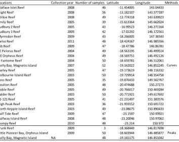
(27) Chapter 2. Abstract The advent of next-generation sequencing has brought about an explosion of single nucleotide polymorphism (SNP) data in non-model organisms; however, profiling these SNPs across multiple natural populations still requires substantial time and resources. Here, I introduce two cost-efficient quantitative High Resolution Melting (qHRM) methods for measuring allele frequencies at known SNP loci in pooled DNA samples: the “peaks” method, which can be applied to large numbers of SNPs, and the “curves” method, which is more labor intensive but also slightly more accurate. Using the reef-building coral Acropora millepora, both qHRM methods can recover the allele proportions from mixtures prepared using two or more individuals of known genotype. Furthermore, advantages of each method over previously published methods are demonstrated; specifically, the “peaks” method can be rapidly scaled to screen several hundred SNPs at once, whereas the “curves” method is better suited for smaller numbers of SNPs. Compared to genotyping individual samples, these methods can save considerable effort and genotyping costs when relatively few candidate SNPs must be profiled across a large number of populations. One of the main applications of this method could be validation of SNPs of interest identified in population genomic studies.. 2.1 Introduction Population genomics seeks to link genome-wide genetic variation to evolutionary processes. By querying a large number of individuals for multiple single nucleotide polymorphisms (SNPs) distributed across the genome, polymorphisms with unexpected patterns of genetic differentiation can be identified. These SNPs may be linked to loci under divergent selection between disparate environments (Stinchcombe & Hoekstra 2008). Recent advances in high-throughput sequencing have made it easy to identify large numbers of SNPs in a limited number of individuals (Davey et al. 2011).. 13.

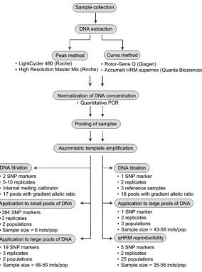
(28) Chapter 2 However, profiling a smaller number of SNPs across many populations, for example to study allele frequencies at specific candidate SNP loci, remains time consuming and expensive if based on individual genotyping. There are many conceptual approaches to determine allele frequencies from pooled samples, including (i) direct sequencing (Bansal et al. 2011; Gautier et al. 2013), (ii) primer extension using pyrosequencing (Lavebratt & Sengul 2006; Doostzadeh et al. 2008), SNaPShot (Norton et al. 2002) or MALDI-TOF mass spectrometry (Werner et al. 2002), and (iii) preferential hybridization or amplification using allele-specific primers, such as TaqMan (Holland et al. 1991), qPCR (Germer et al. 2000), the Illumina GoldenGate platform (Campino et al. 2011), or hybridizing microarrays (Butcher et al. 2004). For a more extensive review of quantitative genotyping technologies, see Sham et al. (2002) and Garvin et al. (2010). Many of these technologies show high correlations between the estimated genotype frequency from the pooled sample and the true allele frequency assessed from genotyping of individual samples, but most require considerable investment of funds and effort for each new SNP assay. While direct sequencing with next-generation sequencing methods is an increasingly popular option, the sequencing of whole genomes, reduced representation libraries (RRL), or even specific amplicons incurs unnecessary costs for research that seeks to investigate the frequencies of a subset of preselected candidate or otherwise potentially informative (“tag” or “proxy”) SNPs across populations. Conventional high resolution melting (HRM) has been established as a very sensitive tool for detecting even low levels of a target allele (Er & Chang 2012). Quantitative HRM methods have been developed in a range of applications Palais et al. 2005), including detection of the adulteration of food or drug products (Mader et al. 2011; Sakaridis et al. 2013a; Sakaridis et al. 2013b; Ganopoulos et al. 2013), methylation. 14.

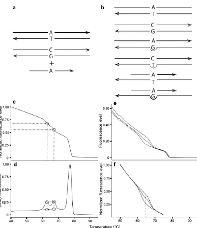
(29) Chapter 2 status (Balic et al. 2009; Malentacchi 2009; Stuopelyte et al. 2013) and species composition in samples over time (Lin & Gänzle 2014). One commonality of these approaches is that they make use of relatively large differences among variants, such as multiple methylated sites within an amplicon, multiple SNP differences among species in the locus of interest or even entirely different genes representing different species. These methods are not sufficiently sensitive to detect frequencies of single SNPs among populations of the same species. The conventional, unlabelled probe version of HRM method of SNP genotyping uses a small oligonucleotide probe to increase the differences in melting temperature between single SNP alleles. It makes use of a dye that fluoresces only when intercalated into duplex DNA structures. First, the SNP-bearing locus of interest is amplified with asymmetric PCR such that an excess of one strand is produced. Next, the short probe that overlays the SNP site itself is added to the reaction. The reaction is subsequently heated, cooled and heated again while the loss of fluorescent signal (i.e. duplex DNA disassociation) is monitored. The melting temperature of the probe-SNP duplex region is dependent on the SNP allele state; a perfect match will have a higher melting temperature than will a mismatch (Zhou et al. 2004). A conventional HRM assay typically seeks to determine whether the probe melting profile contains only the highertemperature component, the lower-temperature component, or both. The main objective of this study is to explore whether the unlabelled probe HRM melting profile can provide quantitative information about frequencies of alternative alleles in a pooled DNA sample. Two versions of qHRM were developed using different dye chemistries, brands of HRM machines and analytical techniques to quantify the relative proportions of each allele. Six experiments were performed using adult. 15.

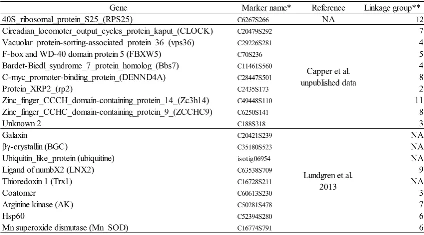
(30) Chapter 2 Acropora millepora corals, an emerging ecological genomics model, to demonstrate the new method’s accuracy.. 2.2 Materials and Methods 2.2.1 Coral collection Adult corals were used in all experiments. For the allele titration and SNP panel validation experiments (peaks method), corals were collected from Trunk Reef (-18.368 S, 146.818 E) and Little Pioneer Bay, Orpheus Island (-18.604 S, 146.486 E), Great Barrier Reef, Queensland, Australia in 2009. Samples used in the Orpheus/Magnetic population comparison experiment (peaks method) were collected from Orpheus Island and Nelly Bay, Magnetic Island (-19.165 S, 146.851 E). Coral samples used to validate the curves method experiments were collected from 28 coral populations, summarized in Table 2.1. All corals were collected under the appropriate Great Barrier Reef Marine Park Authority permits. Table 2.1. Collection year, sample size, latitudes and longitudes of 28 populations. Locations Collection year Number of samples Latitude Longitude Methods Wallace Islet Reef 2008 46 -11.454005 143.04433 Night Reef 2008 56 -13.182107 143.577187 Wilkie Reef 2008 49 -13.774318 143.639923 Emily Reef 2005 39 -15.613364 145.662024 Sudbury 2 Reef 2005 43 -16.99523 146.271164 Sudbury 1 Reef 2005 42 -17.02292 146.172561 Myrmidon Reef 2009 43 -18.266005 147.38343 Kelso Reef 2011 48 -18.424167 146.985556 Rib Reef 2009 47 -18.47786 146.86781 SE Pelorus Reef 2004 49 -18.563195 146.499514 NE Orpheus Reef 2004 49 -18.569751 146.492126 N Fantome Reef 2004 50 -18.659781 146.512061 Nelly Bay, Magnetic Island 2007 52 -19.162022 146.852245 Curves Darley Reef 2005 47 -19.173619 148.116332 Holbourne Island Reef 2003 50 -19.729914 148.354758 Ross Reef 2005 35 -19.876433 149.562767 Boulton Reef 2005 48 -20.474688 150.27273 Goble Reef 2005 49 -20.766017 150.469284 Calder Reef 2003 50 -20.771921 149.617692 21-121 Reef 2005 41 -21.231497 151.383576 High Peak Reef 2003 36 -21.959152 150.691722 North Kepple Island Reef 2003 49 -23.08675 150.890433 Half Tide Reef 2009 47 -23.1597 150.93921 Halfway Island Reef 2008 48 -23.20046 150.97062 Humpy Reef 2010 48 -23.214 150.972 Trunk Reef 2009 3 -18.368449 146.817698 Little Pioneer Bay, Orpheus Island 2009 50 -18.603944 146.485877 Peaks Nelly Bay, Magnetic Island NA 48 -19.165175 146.851042. 16.

(31) Chapter 2. 2.2.2 DNA extraction For the coral individuals used in the allele titration and SNP panel validation experiments (peaks method), genomic DNA was extracted using the DNeasy Blood and Tissue kit (Qiagen) and was eluted into Buffer EB. Individuals sampled from Orpheus and Magnetic Islands (peaks method) and from the 28 populations across the Great Barrier Reef (curves method) were extracted according to the method described in Wilson et al. (2002). DNA concentrations were initially determined using the Nanodrop ND-1000 Spectrophotometer (Thermo Scientific). The workflow of both methods are illustrated in Fig. 2.1. The descriptions of both methods are given in Fig. 2.2 and the following sections.. Fig. 2.1 Flow chart of qHRM, including benchmarking experiments performed for each method.. 17.

(32) Chapter 2. Fig. 2.2 Schematic diagram of qHRM. An individual heterozygous for a particular SNP locus is shown as an example. a) For both methods, the locus is amplified from genomic DNA using asymmetric PCR to generate an excess of the reverse strand. Next, an oligonucleotide probe is added to the reaction. b) The mixture is heated to melt all duplexes apart, and subsequently cooled rapidly to promote unbiased duplex reformation of all possible duplex DNA species. For a biallelic SNP site, this produces six distinct types of duplexes: two perfect-match amplicon duplexes, two mismatch amplicon duplexes, one perfect-match probe duplex, and one mismatch probe duplex. c) For the peaks method, the reaction is heated again to denature all duplexes while the fluorescence of the reaction, which quantifies double stranded DNA, is monitored. d) Next, the negative first derivative of the decreasing fluorescence curve is calculated to transform the curve into a peaks profile. The height of the lowest-melting, mismatched probe duplex peak is divided by the total heights of both probe peaks to yield the frequency of the mismatched allele in the sample. e) For the curves method, the same process was repeated as described for panel c. Three known samples that consist of each genotype (i.e. heterozygote, high-melting homozygote and low-melting homozygote) were used as references. f) Melt curves from the raw channel were normalized by averaging fluorescence value outside a melting phase and forcing the values to be the same for each sample.. 2.2.3 Peaks method. 18.

(33) Chapter 2 The peaks method was developed as a rapid means to quantify SNP allele frequencies across several hundred SNP loci. Briefly, proof of concept was first established using titrated allele frequencies and two SNP markers, then a panel of 384 SNPs was validated using six corals, genotyped individually and as a pool. This panel of SNPs was finally applied to samples of two natural coral populations to detect loci with different frequencies among the reefs.. 2.2.3.1 Pooling In order to convert conventional HRM into a quantitative assay for pooled samples, equal amounts of each individual’s DNA must be added to the initial asymmetric PCR reaction. This DNA normalization step is particularly critical for pooling organisms that may have known or unknown assemblages, infections or symbioses as the relative amounts of target and contaminating DNA can vary among samples. To circumvent these problems, quantitative PCR (qPCR) was used to accurately measure the quantity of coral DNA in individual samples. Primers to amplify the SNP locus C23209S177 (Wang et al. 2009) were used in a conventional qPCR reaction performed under the following conditions using a LightCycler 480 machine (Roche): 5 ng holobiont DNA, 0.1 M each forward and reverse primers, 2 mM MgCl2 and 1x High Resolution Master Mix (Roche) in a 15 l volume. Reactions were heated to 95C for 10 minutes, then cycled 55 times as follows: 40 s at 95C, 40 s at 60C, 40 s at 72C, then cooled to 40C and held for 20s. Concentrations of target DNA were normalized based on differences in quantification cycle (Cq) by assuming that the fold-difference per each Cq unit difference was equal to 1/E, where E is the amplification factor per PCR cycle for the particular primer set (Pfaffl 2001). The accuracy of this approach was verified by reamplifying the adjusted DNA concentrations again with the same primer pair.. 19.

(34) Chapter 2. 2.2.3.2 Internal melting calibrators Though within-plate variation among replicates was low for the peaks method, between-plate variation could shift the melting profile of all duplex DNA species (i.e. for an analysed heterozygote, such species include two perfect-match amplicons, two mismatched amplicons, one perfect-match probe-SNP duplex, and one mismatch probeSNP duplex; Fig. 2.2a,b) by as much as 2C. To accommodate this phenomenon, which occurred only in the peaks method, standard internal melting calibrator primers were included with each reaction in order to provide landmarks in the melting profile. Four oligonucleotide calibrators were designed to form two complementary DNA duplexes with known melting temperatures. They were based on sequences from Gundry et al. (2008) but were adjusted to melt at the slightly lower and higher temperatures of 47.5C and 90C than the published sequences in order to melt well outside of the range of the probe and amplicon duplexes. The 3’ terminal ends of each of the four oligos were modified with an inverted T to block any potential primer extension from occurring. The forward sequence of the low-melting calibrator used is 5’- ATT TTA TAT TTA TAT ATT TAT ATA TTT TT/3InvdT/ -3', while the forward sequence of the high-melting calibrator is 5’- GCG CGG CCG GCA CTG ACC CGA GAC TCT GAG CGG CTG CTG GAG GTG CGG AAG CGG AGG GGC GGG/3InvdT/. The calibrator oligos were included in the initial asymmetric PCR reaction at a concentration of 0.05 M for each of the high-melting oligos and 0.5 M for the low-melting oligos; addition of the calibrators did not interfere with amplification of the target products.. 2.2.3.3 Asymmetric template amplification and melt stage In HRM, the asymmetric PCR stage serves to generate an excess of the amplicon strand that is complementary to the probe. This excess strand can then form a duplex with the unlabelled probe, whereas if it was not in excess it would preferentially bind to. 20.

(35) Chapter 2 the longer, complementary amplicon strand instead. Though some versions of HRM use symmetric PCR, their applications typically involve whole-amplicon melting analysis. In contrast, unlabelled probe HRM, which yields the increased sensitivity necessary for SNP discrimination, requires asymmetric PCR in order to outcompete the amplicon. The asymmetric PCR reaction prior to each assay’s melt stage was performed as follows on the LightCycler 480 (Roche): 5 ng total pooled DNA, 0.3 M reverse primer, 0.067 M forward primer, 0.05 M each high-melting calibrator forward and reverse oligos, 0.5 M each low-melting calibrator forward and reverse oligos, 2 mM MgCl 2, and 1x High Resolution Master Mix (Roche). Reactions were heated to 95C and held for 10m, then cycled as follows: 40 s at 95C, 40 s at 60C, 40 s at 72C for 55 cycles, which, for most SNPs, was at least 10 cycles past the beginning of the reaction plateau. The reaction was then finally cooled to 40C and held for 20 s. Following the asymmetric target amplification, the reaction plates were unsealed and 0.5 M of the oligo probe complementary to the excess reverse strand of the amplicon was added. The plates were resealed and then heated to 95C for one minute to melt all double-stranded DNA species apart. Subsequently, the plates were rapidly cooled to 45C and held for one minute to allow reannealing of all possible probe and amplicon duplexes. Next, the reactions were heated to 95C at the maximum rate allowed by the Roche LightCycler 480 (> 0.02 C/s). During this heating period, the LightCycler 480 monitored the amount of fluorescence over time and collected over 1300 data points over a 50C range, producing a high-resolution graph of the melting profile of each species of duplex DNA in the reaction.. 2.2.3.4 Analysis of denaturation profiles The negative first derivative of the melt stage’s decreasing fluorescence curve were calculated to produce a profile with discrete peaks centred at the melting. 21.

(36) Chapter 2 temperature of each dissociating duplex (Fig. 2.2c,d). Next, a baseline connecting the linear regions bounding the melting peaks was drawn to determine the background rate of dye disassociation. Then, the height of the probe melting peaks above the baseline was measured using a custom [R] script (Supplementary S.1). For pooled reactions, three technical replicates were performed for each locus and sample pair and their relative peak heights averaged. The genotype of a sample was determined by the presence and position of the probe peaks, relative to other samples for the same locus and to the calibrator melting peaks. The frequency of the low-melting allele in a pooled sample was estimated by the contribution of its corresponding melting peak to the total summed height of probe-related melting peaks. Across all SNP assays, a minor allele was called only if it exceeded a frequency of 2%.. 2.2.3.5 DNA titrations To demonstrate a linear relationship between known frequencies of a given allele and the qHRM-estimated frequency estimated from a pooled sample, two individuals homozygous for different alleles of the same SNP were first identified. This experiment was performed for two SNP loci mined from the A. millepora transcriptome, C22162S248 and C45133S676 (Wang et al. 2009). The concentrations of DNA were normalized with qPCR as described above, then the two homozygotes were mixed in different proportions to obtain mixtures that incremented the frequency of the lowmelting allele from 0-100% in 5% or 10% steps (Table 2.2). qHRM was then performed on each mixture with five replicates for each mixture for two independent normalization and mixing trials, for both SNPs assayed. The estimated allele frequencies for all replicates of each mixture were then averaged and compared to the known allele frequencies.. 22.

(37) Chapter 2 Table 2.2. Known frequency mixtures and their qHRM-estimated frequencies of a low-melting allele for three SNP loci: C22161S248; C45133S676; C70S236. Sample batches that were pooled at gradient allelic ratios. SNP C22161S248 # Total replicates Expected freq. of low-melting allele Average qHRM-estimated freq. Standard deviation 10 1 0.9567 0.093 10 0.95 0.8265 0.0481 10 0.9 0.7997 0.057 10 0.85 0.7655 0.0345 10 0.8 0.7148 0.0447 10 0.75 0.6822 0.0541 10 0.7 0.658 0.0396 10 0.6 0.5393 0.1178 10 0.5 0.5164 0.044 10 0.4 0.4035 0.0878 10 0.3 0.3594 0.0505 10 0.25 0.3085 0.0604 10 0.2 0.2925 0.0473 10 0.15 0.2241 0.0493 10 0.1 0.1954 0.0393 10 0.05 0.1424 0.0172 5 0 0 0. SNP C45133S676 # Total replicates Expected freq. of low-melting allele Average qHRM-estimated freq. Standard deviation 5 1 1 0 10 0.95 0.8399 0.0525 10 0.9 0.7404 0.0489 10 0.85 0.6012 0.074 10 0.8 0.5057 0.0621 10 0.75 0.5719 0.0544 9 0.7 0.5316 0.0832 10 0.6 0.4658 0.1022 10 0.5 0.3594 0.0508 10 0.4 0.2882 0.0498 10 0.3 0.2363 0.0618 10 0.25 0.1906 0.0303 10 0.2 0.1634 0.0307 10 0.15 0.1303 0.0233 10 0.1 0.0956 0.0132 9 0.05 0.0613 0.018 9 0 0.0082 0.0106. SNP C70S236 # Total replicates Expected freq. of low-melting allele Average qHRM-estimated freq. Standard deviation 2 1 1 0 2 0.9 0.9138 0.009 2 0.85 0.861 0.0098 2 0.8 0.7738 0.0113 2 0.75 0.7429 0.0212 2 0.7 0.7102 0.016 2 0.65 0.6405 0.0142 2 0.6 0.5858 0.0175 2 0.5 0.5109 0.0176 2 0.5 0.5 0 2 0.4 0.4064 0.0075 2 0.35 0.3608 0.0001 2 0.3 0.3076 0.0029 2 0.25 0.2689 0.0028 2 0.2 0.1983 0.0061 2 0.15 0.1695 0.0024 2 0.1 0.1084 0.0024 2 0 0 0. 23.

(38) Chapter 2. 2.2.3.6 Analysis of 384 loci in six individuals DNA samples from three adult coral individuals sampled from Trunk Reef and three from Orpheus Island were genotyped individually by conventional HRM for 384 loci selected from SNPs previously developed for a previously published coral linkage mapping project (Wang et al. 2009) (Supplementary Table S.2). Following this, the samples were normalized for coral DNA concentration as explained above and pooled to generate a DNA sample with known allele frequencies for each SNP locus. qHRM was performed in triplicate on the pooled sample for the same 384 SNPs. To fully validate qHRM of each SNP in this panel, a validation analysis was done for only data from SNPs for which all six individuals were both successfully amplified and had easily distinguishable peaks when analysed using conventional HRM, and which had clear qHRM peaks greater than 2% of the total fluorescence signal in the reaction (usually relative to the amplicon peak’s height). At least two successful replicates were required for each SNP in the qHRM reactions for analysis to proceed.. 2.2.3.7 Analysis of 384 loci in 98 individuals collected from two locations The peaks method was used to compare allele frequencies in two populations of corals collected from Magnetic Island (n = 48) and Orpheus Island (n = 50). DNA was normalized, pooled according to reef of origin, and qHRM-genotyped in triplicate using a panel of 384 SNPs. Nineteen of these SNPs were further validated by individual HRM genotyping of each individual contributing to the pools. The set of SNPs to validate was selected to represent loci where the low-melting allele was major (8 SNPs) or minor (11 SNPs), loci with small or large minor allele frequencies (11 SNPs with MAF < 0.25; 8 SNPs with MAF > 0.25), SNPs with more than two alleles (7 SNPs with third alleles in one or. 24.

(39) Chapter 2. 25. both populations), and loci selected to span the range of estimated FST values (7 SNPs with FST less than 0.01; 4 SNPs with FST between 0.01 and 0.02; 8 SNPs with FST greater than 0.02, including four of the top seven SNPs with the greatest F ST).. 2.2.3.8 Analysis of genetic subdivision between coral populations SNP allele frequencies were compared between Orpheus and Magnetic populations by plotting the averaged qHRM-estimated frequencies against each reef. FST for each SNP was calculated according to Equ. 1, where p is the frequency of the high-melting allele, q is equal to (1-p), p is the average frequency of p allele between the two populations, and q is equal to (1- p ).. Equ. 1: FST =. ( p1  p2 ) 4 pq. 2. Global FST was calculated by averaging all SNP FST values.. 2.2.4 Curves method The curves method was developed to extend qHRM and demonstrate functionality across another dye chemistry and analytical approach. This method is best suited for highly accurate determination of allele proportions across small numbers of SNPs. It requires the usage of three reference sequences (two homozygous samples and a heterozygous sample) for comparison with an unknown, pooled sample. The curves method demonstrates that reactions are extremely reproducible and robust among different markers and pooled samples. The workflow of the curves method is illustrated in Fig. 2.1. Briefly, the curves method was validated through an initial proof of concept experiment using different known proportions of alleles for a single SNP marker. This.

(40) Chapter 2 marker was additionally validated on three DNA pools made from 43-56 individuals representing distinct coral populations by comparing the true allelic frequency of the pool (revealed by summing the genotypes of each individual) to the qHRM-estimated frequency. Thirdly, reproducibility of this method was investigated by using five SNP markers for pooled samples representing 25 coral populations.. 2.2.4.1 Pooling Each individual sample was amplified individually in an asymmetric qPCR reaction using primers for the locus C70S236 (Wang et al. 2009) under the following conditions using a Rotor-Gene Q machine (Qiagen): 0.1 M forward primer, 1 M reverse primer, 10 ng holobiont DNA, 1x 7.5 l of the Accumelt HRM supermix (Quanta Biosciences) in a 15 l volume. The reaction mixture was heated at 95C for 10 min, then cycled 40 times with the following thermoprofile: 95°C for 40 s, 58°C for 40 s, and 72°C for 40 s. DNA concentrations were normalized according to Pfaffl (2001) as summarized in the Peaks - pooling section. Experiments also contained tubes without DNA template (negative controls).. 2.2.4.2 Asymmetric template amplification and melt stage After normalization of individual samples, each individual was combined into a single pooled sample. The pooled sample was then amplified asymmetrically with the Rotor-Gene Q machine (Qiagen) with the locus C70S236. Next, 1 M of probe complementary to the excess strand was added to each reaction. Then, the reactions were heated to 95C and held for 60 s, rapidly cooled to 45C and held for 150 s, heated again to 95C at a rate of 0.1C/s with a 2 s hold each step, collecting 500 data points in total.. 2.2.4.3 Analysis of denaturation profiles. 26.

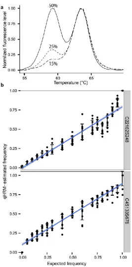
(41) Chapter 2 Because many factors such as pipetting errors causing variations in quantity of fluorescent dye and DNA can affect the relative fluorescence levels among normalized DNA samples, it is important to standardize the fluorescence levels to exclude the noise for accurate allele frequency measurements. Fluorescence values of the SNP-specific melt curves were standardized by selecting regions before and after the probe melting phase where nucleotide differences do not lead to variations in fluorescence level, then averaging fluorescence levels of the selected regions among all samples using the RotorGene Q Series Software 2.0.2.4 (Corbett) in order to mitigate the effects of sample- and SNP-specific variation (Fig. 2.2e). The exclusion of noise through this normalization process allows the direct comparison of melting curves from different reactions. The inclusion of three standard reference samples (positive controls) of known genotype (two different homozygotes and a heterozygote) allows for even small differences in allele frequency to be resolved. These standards set a reference fluorescence level to which unknown samples can be compared for absolute allele frequency quantification (Fig. 2.2f) and also serve to reduce variations between runs. The y-axis point at which the greatest difference in fluorescence between the two homozygotes occurs is used to determine the relative proportion of alleles in an unknown sample as it gives the highest accuracy in estimating allele frequencies (Fig. 2.3). This point should also be near where the inflection point of the heterozygote’s curve falls. But, because the heterozygote can suffer from amplification biases, the position of the inflection point can vary. The accuracy increased by calculating the allele frequency of the unknown sample with respect to the heterozygote rather than simply using the midpoint of the two homozygotes. For example, if an unknown sample has a higher frequency of the high-melting allele (i.e. the unknown’s curve falls above of the heterozygote’s curve and/or the point of the greatest distance between homozygotes),. 27.

(42) Chapter 2. 28. then Equ. 2 can be used to estimate the proportion of the high-melting allele. If the unknown has a higher frequency of the low-melting allele (i.e. the unknown’s curve falls below the heterozygote’s curve and/or the point of the greatest distance between homozygotes), then Equ. 3 should be used to calculate the frequency of the highmelting allele. In both equations, the proportion of fluorescence at the inflection point of the unknown sample (x) relative to the heterozygote (fhet) was calculated. After adjusting for empirical differences between the known heterozygote and one of the known homozygotes (fhigh or flow), the value was added or subtracted from 0.5 to determine the allele frequency of the unknown sample relative to the low-melting homozygote.. Equ. 2: frequency of high-melting allele = 0.5 + 0.5 (. 𝑥−𝑓ℎ𝑒𝑡. 𝑓ℎ𝑖𝑔ℎ −𝑓ℎ𝑒𝑡. Equ. 3: frequency of high-melting allele = 0.5 − 0.5 (. ). 𝑓ℎ𝑒𝑡 −𝑥 ) 𝑓ℎ𝑒𝑡 −𝑓𝑙𝑜𝑤. Fig. 2.3 Standard deviations of differences between estimated and expected allele frequencies across melting temperature range. The standard deviation (i.e. inaccuracy) increased towards either end of the melting temperatures. The smallest standard deviation was observed at the temperatures between 64.4-64.5°C, indicating the highest accuracy in estimating allele frequencies at this temperature range. Consistent with this, the largest difference in fluorescence level between two homozygotes was also observed within the same temperature range for C70S236 marker.. 2.2.4.4 DNA titrations and method validation.

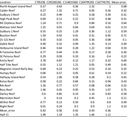
(43) Chapter 2 The use of three reference genotypes per SNP assay and the fluorescence standardization step should theoretically allow for great sensitivity to detect allele frequency differences among pooled samples. To assess this, multiple individuals of each of the three possible genotypes for the locus C70S236 were identified and DNA concentrations of each sample were normalized. DNA samples were then combined into one pool per genotype and mixed in varying proportions to generate a gradient of alleles spanning 0-100% of the low-melting allele by 5-10% increments. The estimated allele frequencies for two technical replicates of each mixture were averaged and compared to the expected allele frequencies (Table 2.2).. 2.2.4.5 Application to large pools of DNA DNA sampled from individual corals sourced from Myrmidon (n = 43), Night (n = 56) and Wilkie (n= 49) Reefs was normalized and individually genotyped using SNP C70S236. Normalized samples were then pooled by population and quantitatively genotyped in duplicate in order to examine the accuracy of the curves method when used with many individuals per pool.. 2.2.4.6 qHRM reproducibility Next, the reproducibility of qHRM on 25 populations sampled along the Great Barrier Reef was evaluated. DNA from 35-56 individuals for each population was pooled, and then curves qHRM was performed on each pool in duplicate for five SNPs (C29226S281, C70S236, C11461S560, C16774S791 and C20479S292), using samples normalized as per above. Consistency between the two replicates was measured by estimating the halfconfidence interval of the difference as follows:. 29.

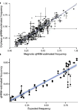
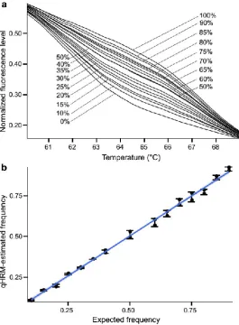
(44) Chapter 2. 30 𝑧 × 𝑆𝐷 𝑚𝑒𝑎𝑛. Standard deviations (SD) and mean values were calculated using fluorescence levels in the temperature range where the largest difference in fluorescence levels between the two homozygotes were observed (Fig. 2.2f). A z value of 1.96 was used so the measure of precision represents half of a 95% confidence interval. Furthermore, the qHRM reproducibility was examined for the 5 markers and 25 reefs by comparing mean errors. Errors in percentage were calculated as follows: Percentage of error between replicates = (. 𝑓1 −𝑓2 ) (𝑓1 +𝑓2 )/2. where f1 and f2 are two replicates of fluorescence data. Geometric means of errors were used as population- and marker-specific errors.. 2.3. Results 2.3.1 Peaks method 2.3.1.1 Allele titrations As an initial proof of concept, a validation analysis was done on DNA from two adult individuals determined to be homozygous for different alleles of the same SNP, mixed in varying proportions to represent a spectrum of allele frequencies. The probe peaks for three allele frequency examples (50%, 25%, 15%) are presented in Fig. 2.4a. For the two SNPs analysed in this way, there was a strong linear correlation between the qHRM estimations and the true proportion (Pearson r = 0.97-0.99). However, the slope of the regression for both SNPs was 0.80 (Fig. 2.4b,c)..

(45) Chapter 2. Fig. 2.4 DNA titrations using the peaks method. a) Probe melting peaks for different allele titrations demonstrating clear resolution among allele frequencies (15%, 25%, 50%). Two homozygotes were mixed in varying proportions to test qHRM using b) SNP C45133S676 (Pearson’s r = 0.97, regression slope = 0.82) and c) SNP C22162S248 (Pearson’s r = 0.99, regression slope = 0.80). The qHRM estimates were tightly correlated to expected frequencies; however, qHRM appears to underestimate the true allele frequency for the low-melting allele for both SNPs considered.. 31.

(46) Chapter 2. 2.3.1.2 Analysis of 384 loci in six individuals To further validate the method, DNA samples from six adult coral colonies from two reefs were individually genotyped for 384 SNPs selected from the coral linkage map using conventional HRM. DNA from these six individuals was pooled and the allele frequency at each SNP was estimated using qHRM. Of the 291 SNPs that passed quality filtering, 54 were homozygous, all of which were correctly identified by qHRM. For 237 polymorphic SNPs, the Pearson correlation between the expected and estimated allele frequencies was 0.89 with a regression slope of 0.94 (Fig. 2.5), qHRM failed to detect polymorphism for eight of the polymorphic SNPs, all of which had minor allele frequencies of 8%, the lowest possible allele frequency in this experiment.. Fig. 2.5 Analysis of 384 loci in six individuals (Peaks method). Six adult corals were HRMgenotyped individually for 384 SNPs, then qHRM-genotyped as a pool in triplicate. The expected allele frequency was calculated by summing the genotypes for each individual (12 alleles possible), and the qHRM-estimated frequencies were calculated as described in the Materials and Methods section. The Pearson correlation between the expected and the qHRM-estimated values is 0.89. The slope of the linear regression is 0.94.. 2.3.1.3 Analysis of 384 loci in 98 individuals collected from two locations. 32.

(47) Chapter 2 To demonstrate that qHRM can identify SNPs with different allele frequencies among real populations, the same 384 SNPs in pooled samples representing the Magnetic Island and Orpheus Island populations of A. millepora were surveyed. These populations are geographically close together but have very different environmental parameters and some degree of genetic separation (FST = 0.041) (van Oppen et al. 2011). Of the 384 SNPs assayed, 261 were represented by at least two technical replicates in each population, including 34 monomorphic loci. Notably, the qHRMestimated allele frequencies for the 261 loci were very similar among populations (Pearson’s r = 0.93, slope = 0.97) (Fig. 2.6a). Global FST between the Magnetic and Orpheus populations using 261 SNPs was calculated as 0.006. The qHRM allele frequency calls for 19 SNPs were further validated by individually genotyping members of each population (total n = 98) using conventional HRM. The Pearson correlation between expected allele frequencies and the qHRMestimated frequencies for these 19 SNPs was 0.93 with a regression slope of 0.77 (Fig. 2.6b). Three of the 19 SNPs from Orpheus Island and two from Magnetic Island populations failed to generate reliable HRM data for one to six individuals, suggestive of a mutation in the HRM primer biding site(s), and therefore were not possible to fully validate. However, it is likely that these missing individuals also failed to contribute to the pooled sample’s allele frequency estimate.. 33.

No results found