University of Southern Queensland
Faculty of Health, Engineering & Sciences
Engineering Correlations for the
Characterisation of Reactive Soil Behaviour for
Use in Road Design
A dissertation submitted by
Peter William Reynolds
in fulfillment of the requirements of
Courses ENG4111 and ENG4112 Research Project
towards the degree of
Bachelor of Engineering (Civil)
i
Abstract
In the field of road design and construction, expansive or reactive soils are problematic materials. Clay minerals within reactive soils are subject to large volume changes when exposed to water, and conversely when they are exposed to prolonged periods of drying.
The surface movements resulting from the wetting or drying of a reactive soil can cause distress to structures that are founded on them. This creates safety and serviceability issues for road users and high maintenance costs to the road authorities and the community.
Whilst there is a body of data and published information on some of the relationships between certain material parameters, a definitive engineer’s guide on the correlations of engineering parameter for expansive soils within Queensland does not appear to exist.
Currently, the primary reference for site classification in respect to the degree of reactivity is the Australian Standard AS2870 – Residential Slabs and Footings. Within this standard, methods are provided to enable an estimation of the range of vertical movement due to swelling and shrinkage. These estimates are based on the Shrink Swell Index (Iss), which is determined by as simple soil test method on an undisturbed soil sample taken from the site of investigation.
ii
Historical data was gathered from reported site investigations carried out on Queensland state road projects from 1995 to 2012. From this data, the relationships between the measures and indices from some of the most commonly used laboratory methods for characterising reactive soils were examined.
iii
University of Southern Queensland
Faculty of Health, Engineering & Sciences
ENG4111/2 Research Project
Limitations of Use
The Council of the University of Southern Queensland, its Faculty of Health, Engineering & Sciences, and the staff of the University of Southern Queensland, do not accept any responsibility for the truth, accuracy or completeness of material contained within or associated with this dissertation.
Persons using all or any part of this material do so at their own risk, and not at the risk of the Council of the University of Southern Queensland, its Faculty of Health, Engineering & Sciences or the staff of the University of Southern Queensland.
This dissertation reports an educational exercise and has no purpose or validity beyond this exercise. The sole purpose of the course pair entitled “Research Project" is to contribute to the overall education within the student's chosen degree program. This document, the associated hardware, software, drawings, and other material set out in the associated appendices should not be used for any other purpose: if they are so used, it is entirely at the risk of the user.
Dean
iv
Certification of Dissertation
I certify that the ideas, designs and experimental work, results, analyses and conclusions set out in this dissertation are entirely my own effort, except where otherwise indicated and acknowledged.
v
Acknowledgments
The author would like to thank the following people for their assistance: to Dr Kazem Ghabraie (University of Southern Queensland) for his technical guidance, feedback and support during this project; to Mr Siva Sivakumar (Department of Transport and Main Roads) for his assistance in the selection of this topic of research and for his permission in allowing access to the data resources of the Department of Transport and Main Roads; to my colleague Mr Jeremy Kirjan, for his encouragement and support; and to my family, for their support and patience in what has been a long wait for the end of this chapter.
Peter Reynolds
vi
Table of Contents
Abstract... i
Limitations of Use ...iii
Certification of Dissertation... iv
List of Figures...viii
List of Tables ... ix
1 Introduction... 1
1.1 Aims and Objectives of the Project ... 2
2 Impacts on Road Performance ... 3
2.1 Distress on Drainage Structures – Case History... 3
2.2 Distress on Road Embankment – Case History... 4
3 Background and Literature Review ... 6
3.1 Properties of Reactive Soils ... 6
3.2 Mineralogy and Mechanics of Volume Change ... 7
3.3 Soil Suction ... 9
3.4 Active Depth... 13
3.5 Applied Stress... 14
4 Laboratory Methods for Measuring Reactivity... 14
4.1 Laboratory Measurements... 14
5 Predictions of Surface Movement using AS2870 ... 26
5.1 General ... 26
5.2 Instability Index... 27
5.3 Changes in Soil Suction ... 28
5.4 Previous Assessments of Test Parameters with Shrink Swell Index... 28
6 Analysis of Historical Data ... 29
6.1 General ... 29
6.2 Method of Analysis ... 30
6.3 Sample Population Statistics ... 32
6.4 Statistic Relationships ... 33
vii
7.1 General ... 33
7.2 Correlation of Individual Parameters and Shrink Swell... 34
7.2.1 Correlation of Shrink Swell Index and % Passing 0.075mm... 34
7.2.2 Correlation of Shrink Swell Index and % Passing 0.002mm... 35
7.2.3 Correlation of Shrink Swell Index and Liquid Limit ... 36
7.2.4 Correlation of Shrink Swell Index and Plasticity Index... 37
7.2.5 Correlation of Shrink Swell Index and Linear Shrinkage ... 38
7.2.6 Correlation of Shrink Swell Index and Weighted Plasticity Index ... 39
7.2.7 Correlation of Shrink Swell Index and Weighted Linear Shrinkage ... 40
7.2.8 Correlation of Shrink Swell Index and CBR Swell ... 40
7.2.9 Correlation of Shrink Swell Index and Soil Suction... 42
7.2.10 Correlation of Shrink Swell Index and Swelling Pressure... 43
7.2.11 Correlation between shrink swell index and CEC ... 44
7.3 Correlation of Combined Parameter Functions and Shrink Swell Index ... 44
7.3.1 Correlation of Shrink Swell Index and (LS + CBR Swell) ... 45
7.3.2 Correlation of Shrink Swell Index and “Combined Reactivity Index” ... 46
7.3.3 Correlation of Shrink Swell Index and (LS/CBR Swell) Ratio ... 47
7.4 Summary of Correlation Analysis ... 48
8 Conclusions... 48
8.1 Major Outcomes and Key Findings... 48
8.2 Recommendations for Further Work... 50
9 List of References ... 52
Appendix A Project Specification... 60
Appendix B Tabulated Test Data... 62
Appendix C Project Aims and Objectives ... 75
Appendix D Project Methodology ... 77
Appendix E Assessment of Consequential Effects... 81
Appendix F Risk Assessment... 84
Appendix G Resource Analysis ... 87
viii
List of Figures
Figure 1 - Distribution of Cracking Clays within Queensland (Main Roads 2000) ... 2
Figure 2 - Image of damaged abutment wall of culvert at East Warianna Creek ... 4
Figure 3 - Location of distressed embankments on Bruce Highway, Yandina... 6
Figure 4 - Diagram of the structure of a montmorillonite layer (Al-Omari 2000) ... 8
Figure 5 - Comparison of mineralogical structures of kaolinite and montmorillonite (Farris) . 8 Figure 6 - Phase diagram showing soil particles and water in void space... 9
Figure 7 - Diagram of soil water potential energy states (Or et al 2005) ... 10
Figure 8 - Idealised water content profiles within active depth zone (Nelson et al 2001)... 13
Figure 9 - CBR test specimens with swell measurement apparatus (Walters 2008) ... 16
Figure 10 - Hydrometer Testing (Earl 2005) ... 17
Figure 11 - Soil consistency with increasing water content (Sivakugan 2000) ... 17
Figure 12 - Apparatus for Casagrande liquid test (Earl 2010)... 19
Figure 13 - Apparatus for fall cone liquid limit test (TMR 2013) ... 19
Figure 14 - Plastic limit test specimens adjacent to 3mm diameter guide rod (Earl 2010) ... 20
Figure 15 - Soil specimen in linear shrinkage test mould (Main Roads 2008)... 20
Figure 16 - Core shrinkage specimen ... 23
Figure 17 - Apparatus (Oedometer) for swell tests... 24
Figure 18 - Image showing filter paper and soil specimen for suction test (Bulut 2001)... 25
Figure 19 - Predicted surface movement compared to observed surface movement (Fityus 2005) ... 28
Figure 20 - Site locations referenced by TMR technical reports ... 31
Figure 21 - Linear regression plot of % passing 0.075mm and shrink swell index... 35
Figure 22 - Linear regression plot of % passing 0.002mm and shrink swell index... 36
Figure 23 - Linear regression plot of liquid limit and shrink swell index ... 37
Figure 24 - Linear regression plot of plasticity index and shrink swell index... 38
Figure 25 - Linear regression plot of linear shrinkage and shrink swell index... 39
Figure 26 - Linear regression plot of weighted plasticity index and shrink swell index ... 40
Figure 27 - Linear regression plot of weighted linear shrinkage plot and shrink swell index. 41 Figure 28 - Linear regression plot of CBR swell and shrink swell index... 42
Figure 29 - Linear regression plot of soil suction and shrink swell index ... 43
Figure 30 - Linear regression plot of swelling pressure and shrink swell index... 43
Figure 31 - Linear regression plot of linear shrinkage + CBR Swell and shrink swell index . 45 Figure 32 - Linear regression plot of CRI and shrink swell index... 47
ix
List of Tables
Table 1 - Suction values corresponding to certain soil states (Lopez et al 1996)... 12
Table 2 - Guidelines for interpreting strength of relationships (Crewson 2006) ... 32
Table 3 - Modified guidelines for interpreting strength of relationships (including R2) ... 32
Table 4 - Summary of statistical properties of sample data... 33
1
1
Introduction
In the field of road design and construction, expansive or reactive soils are problematic materials. The clay minerals within reactive soils are subject to large volume changes when exposed to water, and conversely when they are exposed to prolonged periods of drying. For some clay minerals, such as montmorillonite, the volume change due to the absorption or removal of water can be as much as 30%. This can result in resulting surface movements of up to (and sometimes greater than) 75mm1, causing distress to the structures founded on them resulting in safety and serviceability issues for road users and high maintenance costs to the road authorities and the community.
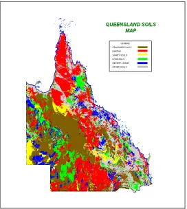
Expansive soils are widely distributed over almost all geographical locations in the world. In Queensland, expansive or reactive soils are referred to by soil scientists as “Cracking Clays” or, more commonly, as “Black Soils” (Dept of Main Roads Qld, 2000). The distribution of these Cracking Clays by land area covers approximately one third of the state. Figure 1 below illustrates the extent of these types of soils within Queensland, based on geological soil mapping.
It is important to properly characterise the properties of expansive soils prior to construction to minimise their impact on the long term performance of infrastructure.
In the analysis and testing of expansive soils, there are various measures and indices used by road designers, and pavement/geotechnical engineers to predict behaviour during the service life of road infrastructure such as pavements, embankments and culverts. Parameters such as CBR Swell, Shrink Swell Index, soil suction, weighted plasticity index, swelling pressure, weighted linear shrinkage, as well as clay content, cation exchange capacity are regularly used.
1
2
Figure 1 - Distribution of Cracking Clays within Queensland (Main Roads 2000)
Whilst there is a body of data and published information on some of the relationships between certain material parameters, a definitive engineer’s guide on the correlations of engineering parameter for Queensland soils and climatic conditions does not appear to exist. Whilst it is acknowledged that to comprehensively characterise the expansive behaviour of all Queensland soil types is beyond the scope of this project, it is hoped that some useful relationships may be identified during the course of the research.
1.1
Aims and Objectives of the Project
3
between the key indicators of reactive soil behaviour will be identified and quantified for future use as guides in the design of roads using these materials.
The objectives of this project can be summarised as follows:
• To understand the nature of expansive soils and their properties
• To identify by research, the key measures of reactive soil behaviour used by
engineers in road construction.
• To investigate and quantify any relationships that may exist between the key
measures.
• To establish a ranking of reliability for the key measures of reactive soil
behaviour.
• To develop guidelines to assist road designers in the identification and
characterisation of reactive soils during the site investigation phase of road construction projects.
2
Impacts on Road Performance
The key elements of a road that are at most risk of damage due to reactive soils are primarily structures on shallow foundations, such as culverts, and pavement layers. The use of reactive soil as fill materials in embankment construction also poses a significant risk for long term performance, if adequate controls are not implemented.
The following section of this report will illustrate by case history, the damaging effects of reactive soil, if the designs do not adequately account for the properties of these materials.
2.1
Distress on Drainage Structures – Case History
4
abutment, wing and pier walls2. Figure 2 below shows the extent of the distress on the culvert.
The distress to the culvert had rendered the structure unsafe, and resulted in its replacement. Actions required to replace the culvert included the construction of a temporary side track, demolition of the existing culvert, removal of the reactive soil to a depth below the zone of influence of the reactive soil, and a replacement of this soil with non-reactive/stable fill. A new culvert base was constructed complete with new concrete culvert cells. It was estimated that the final costs of the replacement works were in the order of $500000.
Based on testing of soil samples taken from the site, it was determined that the cause of the cracking to the structure was due to the stresses imposed on the structure as a result of the shrinking and swelling of the foundation soil as a result of seasonal moisture variations.
Figure 2 - Image of damaged abutment wall of culvert at East Warianna Creek
2.2
Distress on Road Embankment – Case History
Another example of the problems reactive soil can cause to road construction is when they are used as embankment fill. In this example, the approaches to a railway overbridge on the Bruce Highway at Yandina in Queensland, were constructed in 1997-19983. The embankments (maximum height 9m) were
2
MR2469 Department of Transport and Main Roads (2011)
3
5
constructed from local soil materials sourced from a site near to the railway crossing.
Shortly after the completion of construction, longitudinal cracks were observed on the outside of the edge of the concrete pavement wearing course. These cracks were sealed with polystyrene bitumen, however, the cracking continued. Due to concerns about the possible major damage to the concrete pavement, a site investigation was carried out to determine the cause of the cracking. Samples of the embankment were tested in the laboratory and found to have high shrink swell properties. A review of the construction records found that the embankment fill had not been placed in accordance with the road authority’s technical guidelines on construction of expansive clay embankments.
The cause of the cracking was found to be as a result of the shrinkage of the clayey soils within the embankment fill due to a prolonged dry period post construction. It was proposed that the steep embankment batters (1V:1.5H) enabled the drying to occur more rapidly than wound normally be expected. In addition, the flanks of the embankment were not constructed of material suitable for protecting the embankment core from fluctuating moisture contents, due to climatic variations.
The adopted remediation action taken to repair the embankment was to flatten the existing batter slopes using non-expansive soil (1V:2.5H). The estimated total cost of the final repairs to the embankment was approximately $750000.
6
Figure 3 - Location of distressed embankments on Bruce Highway, Yandina
3
Background and Literature Review
3.1
Properties of Reactive Soils
Expansiveness or reactivity is a property of a soil to undergo large volume changes when subject to the actions of wetting and drying. Consideration of the mechanism of interaction between water and reactive soils show that the three most important components are mineralogy, the change in moisture content or suction due to climatic conditions (atmospheric changes), and the stress applied to the soil.
Fine grained soils (eg clayey soils) are known to have a greater potential for reactivity than coarse grained soils (eg soils and gravels). For fine grained soils, the type and proportion and type of clay mineral present influences the potential for reactivity. For example, soils with a high proportion of clay mineral montmorillonite are known to exhibit the very high amount of reactive behaviour.
7
known as soil suction. The drier the soil, the greater the suction, and potential for absorption of moisture. 4
The depth within a soil at which a stable or equilibrium water content can be found is known as the Active Depth or Zone of Seasonal Fluctuations. Soil above the Active Depth is subject to changes in water content and soil suctions, due to climatic conditions; specifically the seasonal cycles of wetting and drying, which influence the degree of reactivity of the soil.
In addition to these intrinsic properties, the magnitude of the stresses applied to the soil by overburden or, for example, embankment loading, also governs the degree to which the soil can react. Problems of volumetric movement and swelling pressure on elements of road infrastructure only arise when the expansiveness is unable to be suppressed.
3.2
Mineralogy and Mechanics of Volume Change
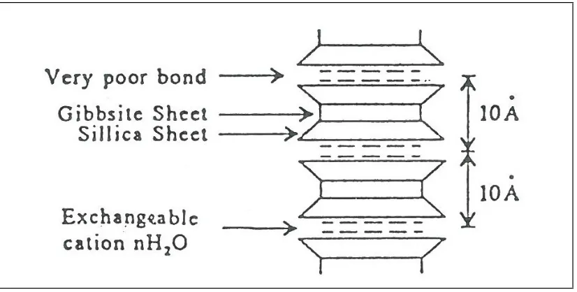
The type of clay mineral is largely responsible for determining the intrinsic expansiveness of the soil. Kaolinitic clays are relatively non-expansive whilst the more expansive clays are smectite clays, also known as montmorillonite clays. The formula for the chemical composition of montmorillonite is Al4Si8O20(OH)4.nH2O
The structure of the clay particles consists mainly of three (3) layers, octahedral sheet, usually occupied by aluminium or magnesium (gibbsite) sheets sandwiched between two sheets of tetrahedral silicon (silica) sheets to give a two (2) to one (1) lattice structure5. This network typically allows water to enter to the centre of the clay particle and be retained for long periods of time (Figure 4). The swelling occurs due to the poor electrostatic bonds between the silica sheets, enabling
4
Nelson et al. (1992)
5
8
[image:18.595.109.522.112.321.2]osmotic pressures to build up and allow for water molecules to be absorbed between the sheets6.
Figure 4 - Diagram of the structure of a montmorillonite layer (Al-Omari 2000)
By comparison, kaolinite, which exhibits little expansive properties, comprises a one to one lattice structure Figure 5 and has a much lower affinity to absorb or retain water molecules within its lattice.
Figure 5 - Comparison of mineralogical structures of kaolinite and montmorillonite (Farris)
6
[image:18.595.108.462.444.663.2]9
This retention is responsible for the movement associated with expansive materials in road construction.
3.3
Soil Suction
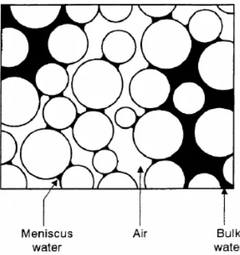
A volume of soil is comprised of solid particles and void space. The void space can be filled with aid and water. When the void space of a soil is completed filled with water, it is said to be saturated. Conversely, when the void space is only partly filled with water, it is said to be in an unsaturated state.
[image:19.595.218.392.359.544.2]The mechanics of the way in which the soil will behave in the unsaturated state, is governed by the inter-particle forces, the air and water pressures within the void space, and the surface tension arising from the interactions of the water and air within the voids. Figure 6 below shows a phase diagram of an unsaturated soil.
Figure 6 - Phase diagram showing soil particles and water in void space
10
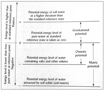
the free energy of water is high (eg standing water table) to one where the free energy is low (a dry soil), is referred to the total soil water potential.
The key components that comprise the total soil water potential are the Matric potential, the Osmotic potential, the potential due to Gravitational forces, and the Pressure potential, due to applied pressures or stresses on a soil.7
[image:20.595.127.485.358.670.2]The Matric potential is the energy associated with the attraction of water by the particles within the soil; Osmotic or solute potential describes the energy associated with the attractive forces within a soil due to water containing salts. Gravitational potential relates to the energy associate with water at an elevation, and pressure potential describes the energy due to any applied stresses to the soil.
Figure 7 below shows graphically the soil water energy states.
Figure 7 - Diagram of soil water potential energy states (Or et al 2005)
The total soil water potential can be expressed in the following equation:
7
11
(Or, Tuller and Wraith)
Where
= The total soil water potential, in centimetres = The matric potential, in centimetres
= The osmotic (solute) potential, in centimetres = The pressure potential, in centimetres
= The gravitational potential, in centimetres
In practical terms, the primary forces acting on soil water held within a rigid soil matrix are: (i) matric forces resulting from interactions of the solid phase with the liquid and gaseous phases (matric potential) and (ii) osmotic forces (solute potential) owing to differences in chemical composition of soil solution.
As stated above, the matric potential is caused by a difference between the air and water pressures within the pore space within the soil.
This is expressed as the simplified equation:
(Or, Tuller and Wraith)
Where
= pore air pressure, in centimetres = pore water pressure, in centimetres
Generally, soil water potential is referred to as total suction terms, and is expressed as:
12
Methods of expressing suctions - there are two units to express differences in energy levels of soil water:
pF Scale: The soil water potential (total suction) is measured in terms of the height of a column of water required to produce necessary suction or pressure difference at a particular soil moisture level. The normal range of the values of suction is wide. Suction is usually expressed as a logarithm of the height of water column (cm) to give the necessary suction, in units of picoFarads (pF); ie
(Or, Tuller and Wraith)
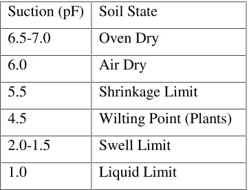
Lopes and McManus (1996) published indicative values relating to specific soil states and are presented in Table 1 below.
Atmospheres or Bars: It is another common mean of expressing suction. One atmosphere (one bar) is the average air pressure at sea level. If the suction is very low as occurs in the case of a wet soil containing the maximum amount of water that it can hold, the pressure difference is of the order of about 0.01 atmospheres or 1 pF equivalent to a column of water 10 cm in height. Similarly, if the pressure difference is 0.1 atmosphere the pF will be 20. Soil moisture constants can be expressed in term of pF values. A soil that is saturated with water has PF 0 while an oven dry soil has a pF 7.
Suction (pF) Soil State 6.5-7.0 Oven Dry
6.0 Air Dry
5.5 Shrinkage Limit 4.5 Wilting Point (Plants) 2.0-1.5 Swell Limit
[image:22.595.208.389.570.708.2]1.0 Liquid Limit
13
3.4
Active Depth
For the problematic behaviour of reactive soils to manifest itself, the soil must be subject to prolonged periods of wetting or drying. If the moisture content within a soil is constant, there is stability. Conversely, where the strata are subject to seasonal fluctuations of soil moisture, the volumetric changes are observable.
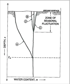
[image:23.595.167.448.285.621.2]Figure 8 shows a number of idealised water content profiles for a problematic reactive clay soil. Profile A demonstrates a water content profile in a uniform soil at an undeveloped site in a dry climate. Below some depth (Depth Zs) an equilibrium water content exists. This is referred to as the Active Zone.
Figure 8 - Idealised water content profiles within active depth zone (Nelson et al 2001)
14
If the ground surface is subjected to temperature fluctuations such as due to summer and winter climates, the water contents in the zone affected by temperature changes will fluctuate about Profile B. Profile C would be typical of wet climatic conditions and Profile D would be typical for dry climatic conditions. The zone in which temperature effects occur, and depths below that in which climatic effects can change the water content define the zone of seasonal fluctuation. The depth of this zone would be less than or equal to the depth Zs (Nelson et al. 2001).
3.5
Applied Stress
The applied stress depends on the structural design and the embankment geometry. The embankment material will act to suppress vertical movement. The amount of overburden required to suppress movement depends on the expansiveness of the soil, and the active depth, as described above.
4
Laboratory Methods for Measuring Reactivity
4.1
Laboratory Measurements
Below is a summary of the most commonly used laboratory methods in the determination of soil reactivity for roads (Pritchard et al. 2000)
• California Bearing Ratio - % Swell
• Particle Size Distribution using Hydrometer (% Finer that 2 um) • Atterberg Limits (Liquid Limit, Plasticity Index, Linear Shrinkage) • Weighted Plasticity Index
• Weighted Linear Shrinkage • Shrink Swell Index
15
California Bearing Ratio (CBR) - % Swell
CBR tests were developed in 1952 to assess the strength of pavement subgrades (Lacey, 1998). California Bearing Ratio is defined as the ratio of force required to cause a circular plunger of 1932mm2 area to penetrate the material for a specified distance expressed as a percentage of a standard force (Main Roads 2002). Test specimens are prepared from passing 19.0mm material using a compactive effort of 596 kJ/m3. They are then tested either in a soaked or unsoaked condition.
The method allows for the determination of CBR Maximum Dry Density (MDD) and CBR Optimum Moisture Content (OMC) as well as the optional determination of swell and post penetration moisture content (Main Roads 2002).
This test can be used to simulate climatic conditions and estimate the potential swell behaviour of expansive clays in its natural state (Fox 2002).
The part of the test that is primarily used as a measure of reactivity is the percentage of swelling measured at the completion of the 4 day soaking period. This is performed by using a dial gauge mounted on a frame which, when placed on top of the CBR mould, aligns the dial gauge centrally over a measuring point. This measuring point is placed on top of the compacted sample, prior to the mould and soil being placed in the water bath for soaking.
16
Figure 9 - CBR test specimens with swell measurement apparatus (Walters 2008)
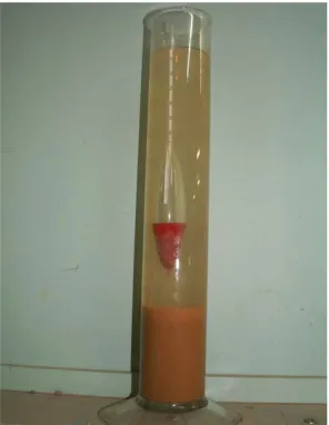
Particle Size Distribution using Hydrometer
Fine grained soils such as silts and clays and have particles smaller than 0.060mm. To determine the grain size distribution of a material <0.075mm sieve the Hydrometer method is commonly used. This test is important in determining the amount of clay present in a soil structure, therefore detailing the amount of plasticity and potential swell the material possesses.
Soil is mixed with water and a dispersing agent, stirred vigorously, and allowed to settle to the bottom of a measuring cylinder. As the soil particles settle out of suspension the specific gravity of the mixture reduces.
An hydrometer is then used to record the variation of specific gravity with time. By relating Stoke’s Law, velocity of a free falling sphere to its diameter the test data is reduced to provide particle diameters and the percent weight of the sample finer than a particular particle size.
17
Figure 10 - Hydrometer Testing (Earl 2005) Atterberg Limits
In the year 1911 Atterberg proposed the limits (liquid limit LL, plastic limit PL
and shrinkage limit SL ) of consistency in an effort to classify the soils and understand the correlation between the limits and engineering properties like compressibility, shear strength and permeability (Casagrande, 1932).
The limits represent the water holding capacity at different states of consistency. The limits are the more prominent procedures for gathering information on the expansive nature and mechanical behavior of clay soils (Williams, A, 1958).
Figure 6 shows a diagram of the different states of soil consistency with increasing water content, including the Atterberg Limits.
18
A useful set of classification data for identifying the swell potential of expansive subgrades are the liquid limit (LL) and plasticity index (PI). The liquid limit is the water content at which a soil changes from the liquid state to a plastic state while the plastic limit is the water content at which a soil changes from the plastic state to a semisolid.
The Plasticity Index is derived from the plastic limit and liquid limit and is represented by the equation below:
PI = LL−PL ( %) (Head) Where:
PI = Plasticity index (%)
LL = Liquid Limit (%)
PL = Plastic Limit (%)
Liquid Limit (LL)
There are two methods to describe the liquid limit (LL) namely percussion cup method and fall cone method. In the percussion cup method, liquid limit is defined as the moisture content corresponding to a specified number of blows required to close a specified width of groove for a specified length (Casagrande, 1932 and 1958). In Queensland, this test is generally carried in accordance with Australian Standard AS1289.3.1.1
The principle of the determination of the liquid limit from the fall cone method is that the liquid limit corresponds to a value of the depth of soil penetration due to a steel cone of specified mass and dimensions.
19
[image:29.595.221.397.155.283.2]The liquid limit data considered in this study has been determined by both Casagande and fall cone methods, using Australian Standard and Transport and Main Roads methods.
Figure 12 - Apparatus for Casagrande liquid test (Earl 2010)
Figure 13 - Apparatus for fall cone liquid limit test (TMR 2013)
Plastic Limit (PL)
[image:29.595.266.351.326.452.2]20
Figure 14 - Plastic limit test specimens adjacent to 3mm diameter guide rod (Earl 2010)
Shrinkage limit (SL) – Linear Shrinkage Test
The shrinkage limit is the water content dividing the semi-solid and the solid state of the soil. It is the water content at which further reduction in moisture content does not result into a decrease in volume of the soil mass. This test can be determined by Australian Standard and Transport and Main Roads methods (AS1289.3.4.1 and Q106). A sample of fine-grained soil, at approximately the liquid limit of the soil, is placed in a shallow trough-shaped mould of 150mm in length, 25mm wide and 15mm deep. The soil and mould are placed in a low drying temperature oven for 2 hours and then placed in a high temperature drying oven overnight.
The length of dried specimen is measured and the linear shrinkage is calculated as the ratio of the change in length due to drying and the original length.
21
Loaded Swell/ Swelling Pressure Test
The loaded swell test provides an indication of the moisture content, soil strength and surface pressure required to suppress swell of a fully saturated soil. This test is performed on an undisturbed sample of soil in its natural (insitu) state.
The soil is trimmed in a steel ring so as to be confined laterally. It is placed in an oedometer apparatus and inundated with water. It is allowed to swell vertically until it achieves a constant value. This completes the Free Swell test, and from this, the percentage of swelling strain observed from the insitu moisture content to the saturated soil condition can be calculated.
Once swell is complete, a series of vertical pressures are applied to the specimen, consolidating it until it reaches the original height of the specimen. A graph of Voids Ratio (%) and. Pressure (kPa) can be plotted and from this, an estimation of the loading required to suppress expansion can be found. This loading value (in kPa) can then be related to a measurement of soil overburden. All loaded swell data used in this study has been determined using ASTM test method D4546 - 03.
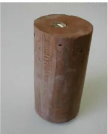
Shrink Swell Index (Iss)
The shrink swell test is composed of companion core shrinkage and swelling tests, carried out on undisturbed soil samples from their initial field moisture contents. The vertically oriented sample is usually obtained from the ground, using a 50-mm-diameter thin-walled tube. The sample is extruded from the tube as a soil core and a suitable portion of the sample is selected for the preparation of a shrinkage core (70–100 mm long) and a swell core (20–25 mm long). Test samples must be from adjacent portions of the core to ensure that water content and both compositional and structural differences are minimized. The test is carried out in accordance with Australian Standard AS1289.7.1.1.
22
Shrinkage Test—This component of the test is identical in procedure to the core shrinkage test, although fewer measurements are required as the shrink-swell index is based on the oven-dried state. A shrinkage core, 45–50 mm in diameter and a length of 1.5–2 diameters, is trimmed from the soil sample. Where possible, it is selected and trimmed to be free of major structural defects and loose material. Initial dimensions and mass are recorded. Small pins are added to each end as reference points to facilitate consistent measurements of sample length as drying proceeds.
The shrinkage core is firstly air-dried. Regular measurements of length and mass are taken until shrinkage ceases. The core is then oven-dried to a constant mass at 105–110
Throughout the drying process, the core is kept in a shallow tray, so that any crumbs that become loose during the test are not lost, as this would affect moisture content calculations.
Swelling Test—this involves a simplified oedometer test in which the sample (of measured mass) is installed in a steel ring, (of measured volume; usually around 20 mm high and 50 mm in diameter) and placed in a consolidation apparatus. A gauge to monitor the sample height is then zeroed under a nominal seating pressure of 5 kPa. A load of 25 kPa or the estimated in situ overburden pressure (whichever is greater) is then applied for 30 minutes to record any initial settlement or seating adjustment. This displacement is used to correct the initial sample height for determination of swelling strain.
23
The initial water content is determined from the sample trimmings, and the final water content is measured from the extracted sample at the end of the test. In the sample preparation process, particular care is taken to ensure that the sample neatly fills the sample ring, as voids and recompacted or remolded portions will accommodate internal adjustments in the volume of the sample and hence, affect the realized vertical swell. Shrinkage strains and swell strains, measured in the respective tests, are then combined to give a shrink-swell index (Iss). 8 This is given by the following equation, (as per AS1289.7.1.1):
2 1.8
sw sh
ss I
∈ ∈ +
= in %/pF
Where
sh
∈ =shrinkage strain in %
sw
∈ =swelling strain in %
The factor of 1.8 is a constant that is adopted for all Australian soils. This relates to the linearly varying part of soil suction changes corresponding to the changes in the axial strains during shrinking and swelling of the soil.
[image:33.595.256.362.460.592.2]Figure 16 - Core shrinkage specimen
8
24
Figure 17 - Apparatus (Oedometer) for swell tests
Soil Suction – Filter Paper Method
This method uses laboratory grade filter paper to measure the matrix suction properties of an undisturbed soil. The filter paper is initially calibrated for suction at different moisture contents.
Once the calibration curve is completed, the test specimen of soil is carefully dissected into a minimum of three layers. Three discs of filter paper (pre-weighed using a balance with an accuracy to 0.0001g) are sandwiched between the soil slices. The sample is tightly wrapped in plastic, ensuring the paper discs are fully in contact with soil only. The soil and filter paper is stored in a sealed container in a controlled temperature environment for 7 days. At the completion of the test duration, the filter papers are individually removed from between the soil slices and their wet mass is measured. The papers are then dried to a constant mass in a drying oven.
The moisture content for each filter paper is then determined, and the average of all three results is calculated. Using the calibration curve for the specified grade of filter paper, the soil suction value is determined from the average filter paper moisture content. The soil suction data used for this study has been determined using BRE Information Paper Method IP 4-93.9
9
25
Figure 18 - Image showing filter paper and soil specimen for suction test (Bulut 2001)
Cation Exchange Capacity
This test method describes the procedures for measuring the soluble and bound cations as well as the cation exchange capacity (CEC) of fine-grained inorganic soils.
Clay minerals in fine-grained soils carry a negative surface charge that is balanced by bound cations near the mineral surface. These bound cations can be exchanged by other cations in the pore water, which are referred to as soluble cations. The cation exchange capacity is a measure of the negative surface charge on the mineral surface. The CEC generally is satisfied by calcium (Ca), sodium (Na), magnesium (Mg), and potassium (K), although other cations may be present depending on the environment in which the soil exists. This test method was developed from concepts described previously in Lavkulich (1981) and Rhoades (1982) In soils with appreciable gypsum or calcite, dissolution of these minerals will release Ca in solution that may affect the measurement.
In this test method, the soluble salts from the mineral surface are washed off with de-ionized water and then the concentration of soluble salts within the extract is measured. The bound cations of the clay are measured by using a solution containing an index ion that forces the existing cations in the bound layer into solution. The total concentrations of bound and soluble cations in this solution are measured.
26
It was found during the collection of the Cation Exchange Capacity data that the suppliers of the testing did not use methodology from well recognized suppliers of standards. Instead it was found that the suppliers used in-house methods based on conventional chemical analysis techniques.
5
Predictions of Surface Movement using AS2870
5.1
General
The Australian Standard AS2870 uses the following equation to predict the characteristic surface movement that a particular layer of soil may produce under seasonal moisture variations:
Where
= characteristic surface movement, in millimeters = instability index in % picoFarads (pF)
= soil suction change averaged over the thickness of the layer under consideration, in picoFarads (pF)
= thickness of layer under consideration, in millimeters
= number of soil layers within the design depth of suction change10
The key parameters within this equation are:
• the instability index ( ) • the soil suction change ( ) • the depth of the clay layer ( )
A point worth noting in reference to the principle behind the determination of the reactivity for a site within then Residential Slabs and Footings Construction standard AS2870, was made by Brown et al. (2002). Specifically, it was observed that AS2870 does not refer to standards tests such as Atterberg limits or linear
10
27
shrinkage to determine reactivity. Instead surface movement (ys) is the primary characteristic used to classify reactive soils. As detailed above, this incorporates the use of soil suction data and the instability index derived from shrink-swell tests into the calculation of surface movement.11
Caunce (2010) observed that the AASHTO guidelines for assessing expansive soils utilise LL, PI and soil suction, whereas Brown (2002) quotes the Australian Standard, AS2870, stating that there are no clear tests to determine clay reactivity. In addition, Brown also postulates that movement is simply a function of mineralogy, proportion of clay, moisture change, loading and lateral restraint.
As such, from these statements and observations above, it can be concluded that the instability index accounts for a number of different properties relating to the reactivity of a soil, within the one single parameter.
5.2
Instability Index
As discussed above, the instability index ( ), in basic terms is a measure of the soil reactivity. This index value is a function of a number of factors including matric and osmotic suction and the stress state of the soil, and the moisture history12. This property can be best approximated by the Shrink Swell Index .
Fityus (2005) reported on the results of a field trial by Cameron in 1989, from a site in South Australia – Gilles Plains. The mean observations of the ground surface movements taken over one wet and one dry cycle were compared against the predicted surface movements based on laboratory values of the shrink swell index of soil taken from the site. The study found that the predicted movements calculated using the shrink swell index were a good estimated of actual ground surface movement. Figure 19 below illustrates these findings.
11
Caunce (2010)
12
28
Figure 19 - Predicted surface movement compared to observed surface movement (Fityus 2005)
5.3
Changes in Soil Suction
Where there is a deficit of water within the soil, this usually gives rise to a negative pore water pressure, known as soil suction. Essentially, the drier the soil, the greater the suction, and potential for absorption of moisture.
Soil suction is a property of soil which is a function of the degree of saturation of the soil and the size of the void spaces within the soil structure. For fine grained soils such as clays, the void space within the soil structure is relatively small compared to that of a granular soil. As a result, when a clayey soil is partially saturated, it is difficult for water to escape from the void space.
5.4
Previous Assessments of Test Parameters with Shrink Swell
Index
29
index weighted by the percentage clay fraction, and similarly with the shrink-swell index and the plasticity index weighted by the percentage clay fraction.
It should be noted that Earl used the a value of the coefficient of determination (R2) > 0.8 as his criterion for determining if the strength of the relationships examined in his work would be useful for the purposes of estimation. Whilst this is considered a reasonable approach, this study has adopted the combined criteria of a coefficient of correlation (r) > 0.7 and a coefficient of determination of (R2) > 0.5 for determining whether a relationship between parameters would be valid in the estimation of the shrink swell index/instability index.
Earl also referenced work by Cameron (1989) which identified a correlation between shrink swell index and linear shrinkage, with a coefficient of correlation of r= 0.76, for a broad range of soils.
In a similar study, Wan et al. (2002) reported a strong correlation between the shrink swell of a soil and liquid limit was reported for volcanic soils from Honolulu.
In research conducted by Earl (2005) a poor correlation was between the shrink-swell index and LS, however, reasonably good correlations were shown between the shrink-swell index and the PI factored by the clay fraction and similarly with the shrink-swell and the PL factored by the clay fraction.
6
Analysis of Historical Data
6.1
General
30
information. The data from these specific reports were extracted and compiled for the purposes of this research.
The reports detailed investigations throughout Queensland’s state road network, ranging from locations from South East Queensland, to the Darling Downs, Central Queensland and North Western Queensland. A map of the sites and the relevant reports to which they relate is shown in Figure 20.
6.2
Method of Analysis
31
Figure 20 - Site locations referenced by TMR technical reports
Using the criteria for strength of relationship from Crewson above, the corresponding values of the coefficient of determination (R2) are presented in Table 3.
32 Range of Coefficient
of Correlation (r) Values Strength of Relationship 0.9 to 1.0
(or -0.9 to -1.0) Very High 0.7 to 0.9
(or -0.7 to -0.9) High 0.5 to 0.7
(or -0.5 to -0.7) Moderate 0.3 to 0.5
(or -0.3 to -0.5) Low
0 to 0.3
[image:42.595.163.432.89.326.2](0 to -0.3) None
Table 2 - Guidelines for interpreting strength of relationships (Crewson 2006)
Range of Coefficient of Correlation (r) Values
Strength of Relationship
Range of Coefficient of Determination (R2) Values 0.9 to 1.0
(or -0.9 to -1.0) Very High
0.81 to 1.0
0.7 to 0.9
(or -0.7 to -0.9) High
0.49 to 0.81
0.5 to 0.7
(or -0.5 to -0.7) Moderate
0.25 to 0.49
0.3 to 0.5
(or -0.3 to -0.5) Low
0.09 to 0.25
0 to 0.3
(0 to -0.3) None
[image:42.595.133.463.377.615.2]0 to 0.09
Table 3 - Modified guidelines for interpreting strength of relationships (including R2)
6.3
Sample Population Statistics
33 <0.075m
m
<0.002m m
LL (%) PI (%) LS (%) WPI WLS Suction - Filter Paper (kPa) Swelling Pressure (kPa) Iss %/pF
CBR Swell - 4 Day Soak
(%)
CBR Swell - 10 Day Soak
(%)
CEC (mEq/100g)
N 183 55 209 208 209 209 188 29 21 100 56 13 10
MEAN 77.8 56.6 67.7 40.7 17.5 3710.7 1604.6 1776.7 321.1 3.0 3.8 4.5 39.2 MEDIAN 82.0 57.0 65.8 38.4 17.4 3443.2 1601.0 2008.0 140.0 2.7 3.3 4.0 28.5 SD 17.3 14.8 23.4 17.5 5.4 1808.5 600.9 937.5 371.2 2.0 3.0 3.0 23.3
CV (%) 22 26 35 43 31 49 37 53 116 68 79 66 59
MIN 16 16.6 19.6 4 2.6 346 225 4 49 0.1 -1.9 0.5 19
MAX 100 88 143 100 29.2 9900 2800 3354 1400 9 11.5 7.9 91
Table 4 - Summary of statistical properties of sample data
Despite the high number of test results extracted from the records, there were a high number of occurrences in which not all laboratory tests were performed on each soil sample. This had the consequence of reducing the number of sets of paired data able to be analyzed through linear regression. For example, in correlating shrink swell index with the soil suction parameter, only 8 pairs of data out of a possible 29 were considered valid, as being obtained from the same representative soil sample. As a result, it was not possible to analyse some relationships, as the sample population was considered too small to be meaningful.
6.4
Statistic Relationships
Table 5 below summarizes the results of the analysis of the relationships between the shrink swell index and the other key parameters. Figures 21 to 33 show the linear regression analysis plots for each pair of parameters compared.
7
Discussion of Results
7.1
General
34
In gathering the data, the main objective was to collect as many sets of data which included the Shrink Swell Index in addition to the other parameters of interest. The purpose of this was ultimately to enable a direct substitution of one of a number of test parameters used to characterize reactive soil properties for the Shrink Swell Index in the AS2870 equation for the determination of the characteristic surface movement,. For this reason, it was important to ensure that
reasonable sample populations of data could be gathered for data sets/pairs including the Shrink Swell Index as the primary parameter.
The limitation of this approach, however, was that the Australian standard test method for the Shrink Swell Index AS1289.7.1.1 was first published in 1992. Indeed, the inclusion of the characteristic surface movement equation in the Residential Slabs and Footings Standard 2870 was only first introduced in 1996. This means that prior to year of publication, the Shrink Swell test did not formally exist and consequently, there is no data older than 1992 of relevance to this study for Queensland or Australia-wide, for that matter. As a result, the period of time considered for data gathering for this study was from 1992 to 2013.
7.2
Correlation of Individual Parameters and Shrink Swell
A discussion of the correlation of each individual parameter with the shrink swell index is presented in following sections of the report. The criteria adopted for this study for assessing whether a particular relationship would be sufficiently reliable to enable the substitution of the shrink swell index with a paired parameter, are based on guidelines given by Crewson (2006), as discussed in Section 5.4. Specifically, where the coefficient of correlation (r) > 0.7 and the coefficient of determination of (R2) > 0.5 for any particular correlation, the relationship is rated of sufficient reliability to be used in the estimation of the characteristic surface movement (ys).
7.2.1 Correlation of Shrink Swell Index and % Passing 0.075mm
35
The size of the sample population for the data is N=67, which appears reasonable to enable the regression to have validity.
[image:45.595.109.503.299.513.2]The resulting trendline is a linear function with r = 0.543 and R2 = 0.2557. Using the criteria for correlation in Table 3, it can be concluded that the data set shows the relationship between the shrink swell index and the percentage finer than 0.075mm is of low to moderate strength. As a result, the percentage finer than 0.075mm would not be a reliable parameter to use for the estimation of the characteristic surface movement (ys).
Figure 21 - Linear regression plot of % passing 0.075mm and shrink swell index
7.2.2 Correlation of Shrink Swell Index and % Passing 0.002mm
The test data used in for the regression analysis are presented in Appendix B. The data is shown plotted in Figure 22 with a regression curve fitted to the data sets.
36
[image:46.595.109.502.257.476.2]The resulting trendline is a linear function with r = 0.417 and R2 = 0.169. Using the criteria for correlation in Table 3, it can be concluded that the data set shows the relationship between the shrink swell index and the percentage finer than 0.002mm is of low strength. As a result, based on this data, the percentage finer than 0.002mm would not be a reliable parameter to use for the estimation of the characteristic surface movement (ys). However, lack of data available for this correlation makes the outcome inconclusive.
Figure 22 - Linear regression plot of % passing 0.002mm and shrink swell index
7.2.3 Correlation of Shrink Swell Index and Liquid Limit
The test data used in for the regression analysis are presented in Appendix B. The data is shown plotted in Figure 23 with a regression curve fitted to the data sets. The size of the sample population for the data is N=69, which appears sufficient to enable the regression to have validity.
37
By using the linear relationship of the line of best fit below, the shrink swell index, can be estimated, and this estimated value can be used for the calculation of the characteristic surface movement, using the AS2870 equation as presented in Section 5.1.
[image:47.595.120.478.215.436.2]Iss=0.0745(LL)-1.611
Figure 23 - Linear regression plot of liquid limit and shrink swell index
7.2.4 Correlation of Shrink Swell Index and Plasticity Index
The test data used in for the regression analysis are presented in Appendix B. The data is shown plotted in Figure 24 with a regression curve fitted to the data sets. The size of the sample population for the data is N=71, which appears sufficient to enable the regression to have validity.
38
the characteristic surface movement, using the AS2870 equation as presented in Section 5.1.
0.0882( ) 2.637
ss
[image:48.595.111.491.128.397.2]I = PI −
Figure 24 - Linear regression plot of plasticity index and shrink swell index
7.2.5 Correlation of Shrink Swell Index and Linear Shrinkage
The test data used in for the regression analysis are presented in Appendix B. The data is shown plotted in Figure 25 with a regression curve fitted to the data sets. The size of the sample population for the data is N=71, which appears sufficient to enable the regression to have validity.
39
Figure 25 - Linear regression plot of linear shrinkage and shrink swell index
7.2.6 Correlation of Shrink Swell Index and Weighted Plasticity Index
The test data used in for the regression analysis are presented in Appendix B. The data is shown plotted in Figure 26 with a regression curve fitted to the data sets. The size of the sample population for the data is N=67, which appears sufficient to enable the regression to have validity.
The resulting trendline is a linear function with r = 0.705 and R2 = 0.523. Using the criteria for correlation in Table 3, it can be concluded that the data set shows the relationship between the shrink swell index and the plasticity index is of high strength. As a result, based on this data, the weighted plasticity index would be a reliable parameter to use for the estimation of the characteristic surface movement (ys). By using the linear relationship of the line of best fit below, the shrink swell index, can be estimated, and this estimated value can be used for the calculation of the characteristic surface movement, using the AS2870 equation as presented in Section 5.1.
0.0009( ) 1.274
ss
40
Figure 26 - Linear regression plot of weighted plasticity index and shrink swell index
7.2.7 Correlation of Shrink Swell Index and Weighted Linear Shrinkage
The test data used in the regression analysis is presented in Appendix B. The data is shown plotted in Figure 27 with a regression curve fitted to the data sets. The size of the sample population for the data is N=67, which appears sufficient to enable the regression to have validity.
The resulting trendline is a linear function with r = 0.679 and R2 = 0.520. Using the criteria for correlation in Table 3, it can be concluded that the data set shows the relationship between the shrink swell index and the plasticity index is of moderate strength. As a result, based on this data, the weighted plasticity index would not be a reliable parameter to use for the estimation of the characteristic surface movement (ys).
7.2.8 Correlation of Shrink Swell Index and CBR Swell
41
Figure 27 - Linear regression plot of weighted linear shrinkage plot and shrink swellindex
In addition, the swelling measurements from tests where the soaked period was 10 days were included in the analysis with the data from tests where the soaking period was 4 days.
The resulting trendline is a linear function with r = 03821 and R2 = 0.607. Using the criteria for correlation in Table 3, it can be concluded that the data set shows the relationship between the shrink swell index and the CBR Swell is of high strength. As a result, based on this data, the CBR Swell would be a reliable parameter to use for the estimation of the characteristic surface movement (ys). By using the linear relationship of the line of best fit below, the shrink swell index, can be estimated, and this estimated value can be used for the calculation of the characteristic surface movement, using the AS2870 equation as presented in Section 5.1.
0.3321( ) 2.382
ss
I = CBRSwell −
42
Z
^
^
/
&
Z^
^
[image:52.595.111.465.72.278.2]^
Figure 28 - Linear regression plot of CBR swell and shrink swell index
7.2.9 Correlation of Shrink Swell Index and Soil Suction
43
Figure 29 - Linear regression plot of soil suction and shrink swell index
7.2.10 Correlation of Shrink Swell Index and Swelling Pressure
The test data used in for the regression analysis are presented in Appendix B. The data is shown plotted in Figure 30 with a regression curve fitted to the data sets. The size of the sample population for the data is N=19, which appears too small to enable the regression to have validity. The following analysis must be viewed in the context of the small sample population.
[image:53.595.108.466.453.674.2]The resulting trendline is a linear function with r = 0.583 and R2 = 0.340. Using the criteria for correlation in Table 3, it can be concluded that the data set shows the relationship between the shrink swell index and the swelling pressure is of low to moderate strength. As a result, based on this data, the swelling pressure would not be a reliable parameter to use for the estimation of the characteristic surface movement (ys). However, lack of data available for this correlation makes the outcome inconclusive.
44
7.2.11 Correlation between Shrink Swell Index and CEC
This relationship was unable to be investigated due to the very low data sets available from the historical Main Roads records. Only four valid data sets were able to be considered for analysis – clearly this sample population is insufficient. As a result the regression analysis between shrink swell index and cation exchange capacity (CEC) was not carried out, and is not presented in this report.
7.3
Correlation of Combined Parameter Functions and Shrink
Swell Index
In the analysis above, only relationships between individual pairs of parameters were examined for potential correlation. However, it is also acknowledged that statistically valid relationships might also exist between combinations of parameters, as related by simple functions.
To explore this proposal in more detail, consideration was given to the method in which shrink swell index is calculated in AS1289.7.1.1.
As detailed in Section 4.1, the shrink swell index parameter is a summation between the strain measured in shrinkage and half of the swelling of the soil specimen, divided by a constant. Fundamentally, the shrink swell index is a function of the shrinkage strain and the swelling strain of the soil.
Linear Shrinkage and CBR Swell and Shrink Swell Index
Of the other parameters considered in this study, the linear shrinkage and the CBR Swell are direct measures of shrinkage strain and swelling strain respectively, despite the obvious differences in the methodology used to obtain these parameters.
45
7.3.1 Correlation of Shrink Swell Index and (LS + CBR Swell)
In an attempt to model the shrink swell index equation, it was decided to at first consider a correlation between the simple summation of the linear shrinkage and the CBR Swell values, and the shrink swell index. The results of this are shown in Figure 31 below, and the values are tabulated in Appendix B.
Z
>^ Z^
^
^
/
&
Figure 31 - Linear regression plot of linear shrinkage + CBR Swell and shrink swell index
It should be noted that the correlation is based on a modest sample population (ie N = 27). However, taking this into account, the correlation between the sum of linear shrinkage and CBR swell was assessed to be of high strength (r = 0.798, R2 = 0.637).
As a result, based on this data, the combination of the linear shrinkage added to the CBR Swell would be a reliable parameter to use for the estimation of the characteristic surface movement (ys). By using the linear relationship of the line of best fit below, the shrink swell index, can be estimated, and this estimated value can be used for the calculation of the characteristic surface movement, using the AS2870 equation as presented in Section 5.1.
0.216( ) 1.202
ss
I = LS+CBRSwell −
46
7.3.2 Correlation of Shrink Swell Index and “Combined Reactivity Index”
Another combination of parameters was investigated for correlation with shrink swell index. The parameters of linear shrinkage and CBR Swell, measuring shrinkage and swelling strain were used in an arrangement similar to the equation used for the calculation of the shrink swell index. This new quantity postulated by the author, is defined by the equation below and is provisionally described by the author as the Combined Reactivity Index (CRI):
( 500)
1.8
LS CBRSwellx
CRI = +
The test data used in for the regression analysis are presented in Appendix B. The data is shown plotted in Figure 32 with a regression curve fitted to the data sets. The size of the sample population for the data is N=25. Despite the modest size of the data set, it appears sufficient to identify trend. However, the population size may not be sufficient to conclusively define the relationship. Hence following analysis must be viewed in this context.
The correlation between the CRI and the shrink swell index was assessed to be of high strength (r = 0.887, R2 = 0.787). This relationship was observed to show the best correlation of all the parameters examined in this study.
As a result, based on this data, the CRI would be a reliable parameter to use for the estimation of the characteristic surface movement (ys). By using the linear relationship of the line of best fit below, the shrink swell index, can be estimated, and this estimated value can be used for the calculation of the characteristic surface movement, using the AS2870 equation as presented in Section 5.1.
0.0017( ) 0.3081
ss
I = CRI −
47
Z
^
^
&
Z /
Figure 32 - Linear regression plot of CRI and shrink swell index
7.3.3 Correlation of Shrink Swell Index and (LS/CBR Swell) Ratio
A third combination of parameters was investigated for correlation with shrink swell index. The CBR Swell and the linear shrinkage were combined in a ratio; specifically CBR Swell/linear shrinkage.
The ratio of the CBR Swell to the Linear Shrinkage was calculated for each set of data in which there was a corresponding shrink swell index test result. The linear regression of the CBR Swell/LS ratio and the shrink swell index is shown in Figure 33, and the values are tabulated in Appendix B.
48
Using Table 3, it can be seen that despite a relatively modest sample population (N=27), the parameters exhibit a high strength relationship (r=0.777, R2=0.603). Thus as the ratio of CBR Swell and linear shrinkage correlates well with shrink swell index for soils over a range of locations, it can be can be cautiously classified as a useful parameter for the purposes of estimation.
By using the linear relationship of the line of best fit below, the shrink swell index, can be estimated, and this estimated value can be used for the calculation of the characteristic surface movement, using the AS2870 equation as presented in Section 5.1.
10.675( / ) 0.684
ss
I = CBRSwell LS +
7.4
Summary of Correlation Analysis
Table 5 below summarises the results of the analysis including the factor and the constants of the regression lines. For the purposes of using the regression equations to calculate an estimation of the shrink swell index, only the parameters in which a high strength relationship was determined should be considered.
8
Conclusions
8.1 Major Outcomes and Key Findings
49
Table 5 - Summary of correlation analysis of all parameters with shrink swell index
This study has also identified some of the laboratory test parameters used to identify and characterise soils with shrink/swell potential. Relatio