A methodology for robust multi-train trajectory planning under dwell-time and control-point uncertainty

This is a repository copy of A methodology for robust multi-train trajectory planning under dwell-time and control-point uncertainty.

White Rose Research Online URL for this paper: http://eprints.whiterose.ac.uk/146289/

Version: Accepted Version

Article:

Goodwin, J., Fletcher, D. orcid.org/0000-0002-1562-4655 and Harrison, R. (2019) A methodology for robust multi-train trajectory planning under dwell-time and control-point uncertainty. Proceedings of the Institution of Mechanical Engineers. Part F: Journal of Rail and Rapid Transit. ISSN 0954-4097

https://doi.org/10.1177/0954409719852242

© 2019 The Authors. This is an author-produced version of a paper accepted for

publication in Proceedings of the Institution of Mechanical Engineers, Part F: Journal of Rail and Rapid Transit. Uploaded in accordance with the publisher's self-archiving policy.

Reuse

Items deposited in White Rose Research Online are protected by copyright, with all rights reserved unless indicated otherwise. They may be downloaded and/or printed for private study, or other acts as permitted by national copyright laws. The publisher or other rights holders may allow further reproduction and re-use of the full text version. This is indicated by the licence information on the White Rose Research Online record for the item.

Takedown

If you consider content in White Rose Research Online to be in breach of UK law, please notify us by

A methodology for robust multi-train trajectory

planning under dwell-time and control-point uncertainty

Jon C J Goodwina_{, David I Fletcher}a,∗_{, Robert F Harrison}b a

Department of Mechanical Engineering, The University of Sheffield, S1 3JD, UK

b

Department of Automatic Control and Systems Engineering, The University of Sheffield, S1 3JD, UK

Abstract

Methods to optimise train movements to maintain time and avoid excessive energy consumption are becoming widely applied, but outcomes remain sen-sitive to uncertainties within the system. In this paper variability in station dwell-times and the points of application of planned train control (traction, coasting or braking) are taken as examples of typical rail system uncertain-ties, and are used to demonstrate an approach to multi-train trajectory op-timisation that is resilient to them.

Trade-offs are explored between highly optimised train trajectories that are vulnerable to perturbation, and less optimal trajectories that are robust to typical disturbances. Beyond dwell and control variations the method has application for the many other common rail network uncertainties, e.g. differ-ences in the traction characteristics of nominally identical trains or variable train loading. Relative to optimisation without consideration of uncertainty,

∗_{Corresponding author}

Email addresses: jonandsarahgoodwin@gmail.com(Jon C J Goodwin),

D.I.Fletcher@sheffield.ac.uk(David I Fletcher),r.f.harrison@sheffield.ac.uk

the approach is shown to find control strategies of substantially increased robustness for the test cases examined, and offers a more principled way to plan a network than the ad-hoc use of recovery time to mitigate everyday operational disturbances.

Keywords: multi-train trajectory optimisation, robust control, energy efficiency, trajectory planning, railway network optimisation, genetic algorithm

1. Introduction

1.1. Background

Owing to increased traffic demands, railway systems in the UK and else-where have become increasingly busy and in some areas their capabilities restrict the volume of people and goods that can be moved1_{. Trains are}

operating at increased frequency but there is often also a desire to minimise travel time and, as a consequence, the system has little slack with an in-creased likelihood that small disruptions can propagate across large parts of the network with disproportionately severe effects.

may not be achievable in practice, i.e. it is not a robust. This has to be mitigated with recovery time built into the timetable, without which oper-ation can become severely degraded as, for example, delays accumulate and cannot be recovered. An example taken from the UK shows a train making 14 station calls on a journey from London to Leeds having a scheduled ex-tended stop of 480s (8 minutes) at its eighth station call. Analysis of 21 days of data2 _{in the period 11}th _{February to 12}th _{March 2019 shows that actual}

dwell time here had a mean of 338s, maximum of 645s and minimum of 225s. The extended dwell was in some cases sufficient to enable recovery of delay that had accumulated by this mid stage of the journey but at other times was under or over generous. Beyond experience of the operator there is no certainty this stage of the journey or scheduled duration of extended stop is the optimum to maintain good service over the whole trip or for other trains routed in the vicinity.

In this paper a method is introduced that attempts directly to impose robustness in planned trajectories through probabilistic variation of CPs and DTs within a genetic algorithm (GA) based, multi-train optimisation process. This is in contrast to simple application of a GA to optimise train trajectory, which has been well covered by previous publications, for example by Chang and Sim, Yang et al. and Goodwin et al.3,4,5_{. The aim is to prove the concept}

network-wide driving strategies of increased robustness, and offers a more systematic way to plan a network than ad-hoc use of recovery time to mitigate everyday disturbances to operation.

1.2. Optimisation in uncertain systems

Most trajectory planning work (for both single and multiple trains) is focused on finding the optimal solution for a predefined timetable. Usually train control seeks to maintain the timetabled traverse time for a length of track, whilst minimising the energy consumption6_{. The problem is}

con-strained by the dynamic performance limits of trains and restrictions on speed and headways. The traditional formulation of the multi-train trajec-tory planning problem can be formalised as:

f(X)→min (1)

where X is a control strategy for all trains on the network, and f(X) is a cost function typically based on the traverse times and energy consumption of all train journeys.

In optimising a rail network it is often assumed that if the optimal control strategy is identified, then its implementation will result in optimal perfor-mance of the system. However, the optimum is likely to lie on the limit of the feasibility boundary and so will be very sensitive to parameter uncertainty or noise7_{. In this context noise refers to the many small uncertainties that}

most current models do not consider but which exist in reality, for example, variations in DT at stations dependent on passenger boarding rate8,9_{. These}

to real operation it is unlikely they will perform as well as expected, and may in-fact result in severely sub-optimal outcomes. Most of these uncertainties fall into two different groups classified by Chen et al.10 _as:

Type 1 - variation (α) in uncontrolled parameters, e.g. variations between nominally identical vehicles, variations in station dwell times.

Type 2 - variation (δ) in control, caused by imperfect application, e.g. variation in locations at which a driver switches between traction, coasting and braking.

Including both Type 1 and 2 variations the problem becomes:

f(X+δ, α)→min (2)

By optimising this system, with noise included, the best result that could be achieved with Equation (1) is expected to be approached but not matched, this deviation being the cost of achieving a robust solution.

To explore the trade-off between cost and increased robustness, an exist-ing multi-train trajectory optimisation study5 _{was utilised with the control}

The uncertainties in DT and CP were quantified as statistical distribu-tions from which values are sampled at each cost function evaluation (full details below). This implies that the value of the cost function will vary stochastically, and therefore a single evaluation could be misleading since it would only examine one combination of uncertainties. A more realistic pic-ture is given by taking the mean of N evaluations for a particular network control strategy, i.e. considering the driving strategies for all trains move-ments that take place. This may be undertaken directly (Equation (3)), or in a GA optimiser may be achieved by increasing the population size. The larger the N used, the better the representation of how the network will really perform for that specific control strategy.

ˆ

F(X) = 1 N

N

X

i=1

f(X+δ, α) (3)

2. Methods

The existing multi-train trajectory planning optimisation method reported previously5,11_{was used as a starting point, focusing on movement of multiple}

2.1. Network and train schedule

The rail network studied (Figure 1) consists of three bi-directional sin-gle track lines, joining four stations. Three trains are considered with the journey schedule given below. Times for traverse and dwell are targets, i.e. maximum traverse times, and minimum DTs, but may be varied by the op-timisation if (for example) an early arrival or extended dwell is beneficial to overall network behaviour. The network traverse times represent 10% slack relative to flat out running and aim to represent a mainline suburban railway operation with stops every 10-12 minutes. It should be noted that the simple network modelled here is being used to explore the optimisation approach, not to represent a specific network.

• Train 1: Mass 665 tonnes. Travels station 1 to 4 (traverse time 675s), calls at station 4 (planned dwell 60s, minimum 30s), terminates at station 2 (traverse time 747s)

• Train 2: Mass 600 tonnes. Travels station 2 to 4 (traverse time 701s), calls at station 4 (planned dwell 60s, minimum 30s), terminates at station 3 (traverse time 605s)

• Train 3: Mass 565 tonnes. Travels station 3 to 4 (traverse time 599s), calls at station 4 (planned dwell 60s, minimum 30s), terminates at station 1 (traverse time 637s)

apply. This allows non-uniform acceleration due to velocity dependence of forces controlling motion to be closely approximated11 _{within a simple}

com-putational approach. Although an analytical calculation could be made for this simple network such an approach rapidly becomes unfeasible for a larger network, so it was decided to use the more scalable time discretisation ap-proach here. The forces controlling motion are the maximum traction force available (360kN, irrespective of velocity), resistance to motion (g), and brake force (h). The velocity dependent quantities are summarised by Equations 4 and 5 in which v is the velocity4_.

g(v) = 11.4 + 0.101v+ 0.001269v2 (4)

h(v) =         

300−0.2v if 0≤v ≤100km/hr 280−1.2(v−100) if 100< v ≤200km/hr 160−0.5(v−200) if 200< v ≤300km/hr

(5)

deterministic features. In combination with the range of train weights these factors provide a variety of behaviour sufficient to test the optimisation of train trajectories to compare cases with and without noise.

V(1,4)(s) = 200km/hr if 15km≤s≤20km V₍₂,4)(s) = 150km/hr if 10km≤s≤13km V(3,4)(s) = 230km/hr if 20km≤s≤23km

(6)

2.2. Optimisation approach

The optimisation process without consideration of noise is fully described by Goodwin et al.5 _{so only a brief summary is provided here. Train}

move-ments are defined by a driving strategy consisting of traction and coasting pairs, so a journey is made up of a series of applications of power (trac-tion) followed by coasting. At the end of the journey braking is triggered to bring the train to a stop at the required station. The locations of transitions between traction, coasting or braking are defined as the CPs. Terminol-ogy varies internationally and the same thing may also be referred to as a switching point, but is distinct from wayside timing points which may also be referred to as CPs in some rail operations. Optimisation is used to establish the best places to make these control changes, although as discussed later the planned positions may not be followed accurately during driving the train. The duration over which traction or coasting is applied determines the speed profile of the train, which must be kept within the line-speed-limit at any location.

usage. During optimisation the performance of the driving strategies was tested by running a simulation of the network and scoring performance using the cost function Equation (7).

cost function =

M

X

i=1

max(0,arrival time - timetabled arrival)

+c

M

X

i=1

energy consumed on journey (7)

where M is the total number of journeys taken on the network across all trains. This trades off delays and energy consumption through the constant, c, by which the relative importance of these factors can be expressed. The value ofccan be modified depending on the relative importance to the oper-ator of timekeeping or energy use, but a fixed value was maintained during the current exploration focused on system variabilities. The cost function used here is an example through which the effects of uncertainties in the system can be explored; alternative cost functions have been developed that are able to account for wider issues than just time and energy, for example by Pavlides and Chow12_.

(phenotype) is initiated, e.g. representing a complete run of timetabled train movements on the network, each characterised by an arbitrary set of problem parameters (genotype), e.g. CP locations and accelerating/coasting/braking actions to achieve the train movements. Each evaluation of the phenotype using its current genotype is scored according to the cost function and the “fittest” (best scoring) individuals are selected for breeding, whereby the genotypes of pairs of fit individuals (parents) are recombined through the mechanisms of crossover (mimicking the combination of DNA strands in sex-ual reproduction) and mutation (mimicking the random variations that can take place in this process). The new generation of “children” then undergoes the same process of evaluation and breeding until a satisfactory solution is reached, determined for instance by a fall in cost below some pre-determined threshold or when local convergence is observed, e.g. via “small” changes in cost from generation to generation. There are many possible ways of implementing genetic operations and the specific choices for this work have been fully described by Goodwin et al.5 _{and so are omitted here for brevity,}

other than to report that a particular feature is its very low risk of becoming “stuck” in cost function local minima rather than approaching the true min-imum. It is worth noting that the means of embedding robustness/resilience in the GA optimisation process could also be applied to other optimisation techniques but here the focus is on GA as there is a large body of work indicating their suitability for addressing train control problems.

Algorithm 1Robust genetic algorithm, illustrated for dwell time robustness 1. Select as training data 50 data-sets for dwell times across the network

during running a timetable

2. For each training data-set n=1..50 simulate the timetable:

(a) Run genetic algorithm (200 generations, population 100) to identify high performing train control strategies to achieve the timetable and energy objectives, defined by Equation (7)

(b) Score each of the final population of train control strategies when applied to simulate the timetable for each of dwell data-sets 1..50, using Equation (3), N=50

(c) Identify the best scoring train control strategy for training data-setn

3. Select the highest performing train control strategy across all 50 train-ing data-sets

specific case of DT or CP uncertainty, on average it will be expected to of-fer the best network performance over a wide range of utilisation conditions without prior knowledge of exactly what these will be.

2.3. Representing DT uncertainty

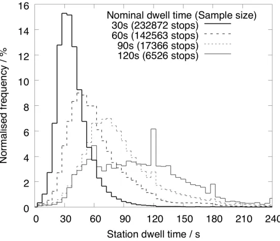
plot-ted in Figure 2, in which two distinct properties can be seen in data covering almost 400,000 station stops on a range of suburban, regional and inter-city routes. First, there is a distribution of DTs achieved around the nominal DT, so modelling just the nominal dwell would clearly be unrealistic. Sec-ond, shorter nominal dwells are associated with a more consistent (narrow) distribution of DTs achieved, whereas longer nominal dwells are associated with greater variability.

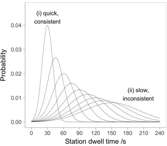
Variation in station DTs was introduced into the model so as to approx-imate real-world behaviour, with the stochastic component normally dis-tributed, and DT truncated to avoid negative waiting timesa_{. To enable}

the uncertainty in DT to be varied smoothly for investigation, the standard deviation in the stochastic component of DT was chosen to always be one third of the mean, resulting in the series of distributions shown in Figure 3, that closely resemble the real-world data in Figure 2. Since DT mean and standard deviation are related in the example cases explored in this paper, DT noise is quantified in the following sections by its mean value. The op-timisation procedure is independent of this distributional choice, so, in real applications, the representation of DT could be tuned to the characteristics of a specific station, line, fleet or known passenger behaviour.

a_{A normal distribution was used for simplicity although the example data in Figure 2}

have a skewed distribution. This has no impact on the consideration of robust trajectory

planning, but developing an alternative distribution to represent DT stochastic component

2.4. Representing uncertain CP application

Adapting the model described by Goodwin et al.5 _{to introduce}

uncer-tainty in CP application into the system was achieved by adding a zero-mean, normally distributed random distance to the position of each CP. Instead of the next control action being applied as soon as the train passed the distance specified in the control sequence the action was applied with the specified level of uncertainty (Figure 4). This distribution could be refined for a spe-cific application, for example, through observation of drivers to understand the spread of early or late applications of control relative to DAS advice. However, as for the DT case, the optimisation procedure developed in this paper is independent of this distributional choice so a simple normal distri-bution is satisfactory. CP noise is quantified in the following sections by its standard deviation. Its inclusion in the representation of train control leads to two closely related situations becoming possible.

First, each time a driving strategy was simulated there was a chance that the trajectories taken do not maintain safe operation, for example by violat-ing the line-speed-limits (Figure 4b). Durviolat-ing the progress of the optimisation such driving strategies were discarded and replaced with a driving strategy probabilistically selected from the previous generation of the optimisation process, this being a safe but sub-optimal driving strategy.

per-forming system with no uncertainties. To screen out these cases the final pop-ulation of potential driving strategies produced by the GA was re-simulated without any noise and any candidates found to be invalid were discarded.

2.5. Optimisation parameters

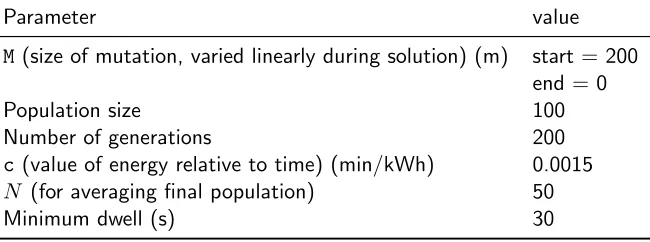
The optimisation parameters used in this investigation are shown in Ta-ble 1, and are identical to those used by Goodwin et al.5_{, except for the}

additions explained above to account for noise. Eiben13 _{observes that}

pa-rameters for a genetic process may have different optimum values throughout the optimisation process, and here it was found that a linear decrease in the size of mutation with each generation yielded improved performance.

Since GAs are not deterministic and the uncertainties being considered add further variability to the system, after completion of each optimisation a further analysis was conducted in which the performance of the chosen control strategy was explicitly estimated, using Equation (3) (N = 500).

3. Results and Discussion

3.1. Baseline: Optimising without noise

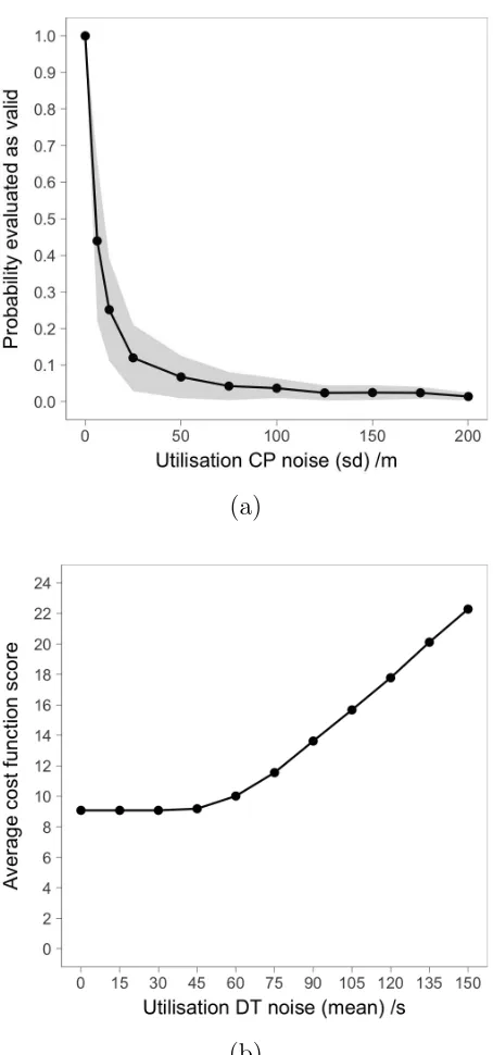
conditions. For the system studied, the mean utilisation DT noise was found to have no effect on the validity of control strategies (no violations of the type shown in Figure 4 occured). This is expected since a DT variation should not adversely change driving behaviour after the train begins to move. Introduction of utilisation CP noise had negligible effect on the cost function scores, and this outcome held for all the different combinations of training noise.

From Figure 5(a) it can be seen that the probability of an optimised control strategy being valid, avoiding Figure 4 type violations, drops quickly as utilisation CP noise increased. The optimised solutions found are very close to the line-speed constraints, and when utilised in a system with no noise they always keep the safety constraints and are therefore considered valid solutions. However, as soon as a small amount of CP noise is introduced during the utilisation of the control strategies the probability of speed-limit violations becomes high, invalidating the control strategies. Far from being surprising, this lack of robustness is exactly the behaviour that would be expected from near optimal solutions to the noiseless problem7_{. By assuming}

certainty in CP application during the optimisation it has produced solutions that are sensitive to CP noise. In reality it would be expected that such speed-limit violations would be avoided by drivers, with the consequence that it would be very difficult or impossible to keep to the scheduled timetable.

strategies that make full use of the timetabled traverse time on each journey (since losses due to air resistance are reduced at lower speeds). If these strategies are followed recovery time is minimised so any late departure will cause a late arrival (with this effect amplified as delays propagate across the network). Below a DT noise with mean of 45s this lack of recovery time is not an issue because the utilisation DT has a very low probability of being greater than the planned DT of 60s. However, above a mean DT noise of 60s the majority of dwells are extended and, since there is minimal recovery time, any increase in DT causes delay and increases the Equation (3) cost function score. Again, by assuming certainty in DTs during the optimisation it has produced solutions that are sensitive to real-world conditions.

3.2. Optimising with CP variability

The second series of optimisations was carried out with different levels of training CP variability during the optimisation process, the results from which are illustrated in Figure 6.

valid control under real conditions comes at a low cost.

3.3. Optimising with DT variability

The next series of optimisations was carried out with different levels of DT uncertainty during the optimisation process, but with no CP uncertainty. The results for training DT noise (mean) = 30, 45 and 135, 150s were found to be almost identical to training DT noise of 0 and 120s respectively so are omitted from Figure 7. For the first case, this is because the training noise level is too low to have a noticeable effect – the vast majority of DT instances are less than the nominal DT used in the system (60s) and therefore rarely affect the actual departure time. In the second case, this is because the training noise level is too high – the optimisation can no longer select genuine improvements in control above the noise. The overall behaviour is that a rise in DT training noise within the limits of what would constitute noise rather than a more major disruption in the real system increases the probability of developing driving strategies that remain valid in real-world conditions, i.e. avoiding Figure 4b type violations.

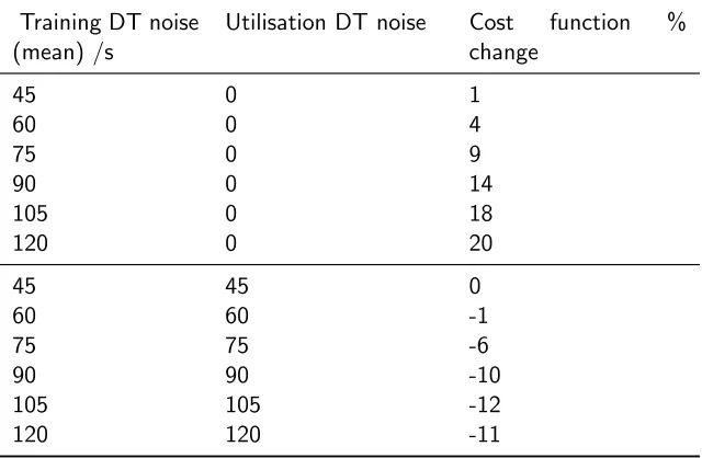
The importance of the training noise matching the noise level at which the solution with be utilised is highlighted in Table 2. The modelling outcomes show that the cost function score when the utilisation DT noise matches the training noise is much lower than when the utilisation DT noise is fixed at zero but the training noise varied. In situations where the utilisation noise levels of a real system are not well known estimates will be needed in the choice of training noise. It follows that all non-robust optimisations make the (usually implicit) assumption that noise levels on all parameters are zero. For many situations, particularly metro applications, this may be an accept-able approximation but it is unlikely to hold in complex, interconnected, stochastic systems such as a busy mainline suburban, regional or intercity rail networks.

metres and a mean training DT noise of 90 seconds). The mean timetabled journey time in the system modelled is 660.7s, calculated across all legs of the timetable detailed in Section 2.1. From Table 3 it can be seen that the mean journey time with 0 0 is 658s, giving a mean recovery time per journey of just under 2.7s. Running with such low recovery time results in 0 0 having the lowest average speed and therefore the lowest energy consumption of the cases in Table 3. At first sight this may be considered a success, since the service is predicted to be is punctual and energy efficient, but when consid-ering robustness this is actually a “brittle” solution, with utilisation noise rapidly leading to sub-optimal performance, as shown in Figure 5.

If the training DT noise is increased to 90s (training noise 0 90) then the mean speed of operation rises and journey traverse time falls to give a mean recovery time of just under 25s on each station to station traverse. This raises the proportion of journeys in which punctual operation can be maintained even where there is a significant probability that DT will be longer than timetabled, but at the cost of running faster and using slightly more energy. Mean recovery time is used here to summarise this behaviour, although the optimisation actually distributes it non-uniformly between journey legs to cope with interaction of services at station 4 (see Figure 1). Interestingly, fast running (in order to build up recovery time) is similar to typical driver behaviour14 _{but in this case has been found by a direct optimisation, which}

has no prior knowledge of existing operational concepts.

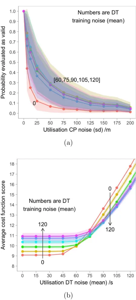
3.4. Optimisation with both CP application and station DT variability

method in this situation. The performance when high levels of CP and DT training noise are present simultaneously is shown in Figure 8. It can be seen that the robustness of control strategies to CP noise at utilisation, indicated by a high proportion of control strategies being valid during ap-plication, is predominantly influenced by the training noise level of CP used during optimisation. In terms of maximising robustness to CP variation the performance of the 100 90 optimisation is very close to the performance of the 100 0 optimisation, indicating that including DT noise at training makes only a marginal difference to performance under CP noise at utilisation. In contrast, Figure 8(b) shows the performance of the 100 90 optimisation is similar, but slightly more costly, than the 0 90 optimisation. Including both training noises simultaneously has led to higher cost function scores than applying DT training noise alone. However, the performance of the 100 90 optimisation is still an improvement over the 0 0 optimisation when utilised at a high level of DT noise. This indicates that the proposed approach for including uncertainty in the optimisation is capable of finding solutions that increase system robustness when two different types of uncertainty exist si-multaneously.

4. Conclusion

predicted in real operation. Non-systematic approaches may address this problem, such as ad-hoc addition of recovery time to timetables, or by driv-ing trains aggressively in an effort to keep to the timetable, but at the cost of excess energy consumption and poor utilisation of trains, crew and network capacity.

A method to consider noise in a multi-train optimisation procedure has been described which seeks to find robust solutions to the multi-train trajec-tory planning problem. For a small demonstration network it is shown to be effective in finding robust control strategies in the presence of two different types of uncertainty: the accuracy of the CPs (i.e. differences in applica-tion point for tracapplica-tion, coasting or braking relative to a planned trajectory), and variation in station DTs. These uncertainties were first considered sep-arately, before it was shown that they could be considered simultaneously in the optimisation, in which case it is predicted that the system will still achieve good levels of robustness. For both types of uncertainty a trade-off was observed between the robustness and the average cost function score at utilisation, which represents a combination of delay and energy costs for the train trajectory solution. The aim here was to explore the concept of including uncertainties in train trajectory planning using a simple network (technology readiness level, TRL, 2-3, proof of concept) in preparation for fu-ture application at TRL 7-9 (operational demonstration). The procedure for including training noise in the optimisation process is generalisable to include the many different uncertainties that can affect railway system operation.

with high levels of uncertainties (large variety of vehicles, stations of differ-ent characteristics). These contrast with metro or underground operations in which there are lower levels of uncertainty (fewer vehicle types, often aiming for flat-out driving to maximise throughput of passengers). The predictions for the example network show that, for best network performance, the train-ing noise used durtrain-ing the optimisation process should reflect the noise level that is expected when the optimised driving strategy is utilised. Planning for a level of uncertainty close to that experienced increases resilience and robustness of the driving strategy without excessive cost.

Directions for further development of the technique include considering different sources of noise (e.g. train resistance coefficients, traction efficien-cies, rail-wheel adhesion levels), and different network topologies and timeta-bles to understand how the method scales with increasing network size. For larger networks implementation using parallel computing on graphics pro-cessing units (GPUs) is expected to offer increased speed of computation.

Acknowledgements

The authors are grateful to Steve Brown at Tracsis Plc for supply of train running data captured from Network Rail open data feeds.

Declaration of conflicting interests

Funding

This research was funded by the Engineering and Physical Sciences Re-search Council, through the E-Futures Doctoral Training Centre at The Uni-versity of Sheffield, EPSRC grant number: EP/G037477/1.

References

[1] Rail Delivery Group, Rail Supply Group, Rail Technical Strategy Capability Delivery Plan, Tech. Rep., Rail Safety and Standards Board, The Helicon, 1 South Place, London,

EC2M 2RB, URL https://www.rssb.co.uk/rts/Documents/

2017-01-27-rail-technical-strategy-capability-delivery-plan-brochure.

pdf, 2017.

[2] Realtime Trains, 1D66 1904 St Pancras International to Leeds, http:

//www.realtimetrains.co.uk, 2019.

[3] C. S. Chang, S. S. Sim, Optimising train movements through coast con-trol using genetic algorithms, IEE Proceedings - Electric Power Appli-cations 144 (1) (1997) 65–73.

[4] L. Yang, K. Li, Z. Gao, X. Li, Optimizing Trains Movement on a Railway Network, Omega 40 (5) (2012) 619–633.

(2015) 1318–1335, URL http://pif.sagepub.com/lookup/doi/10.

1177/0954409715593304.

[6] M. McClanachan, C. Cole, Current Train Control Optimization Methods with a View for Application in Heavy Haul Railways, Proceedings of the Institution of Mechanical Engineers, Part F: Journal of Rail and Rapid Transit 226 (1) (2012) 36–47.

[7] H.-G. Beyer, B. Sendhoff, Robust Optimization - A Comprehensive Sur-vey, Computer Methods in Applied Mechanics and Engineering 196 (33-34) (2007) 3190–3218.

[8] G. de Ana Rodriguez, S. Seriani, S. Holloway, Impact of Platform Edge Doors on Passengers: Boarding and Alighting Time and Platform Be-havior, Transportation Research Record: Journal of the Transporta-tion Research Board 2540 (2016) 102–110, URL https://doi.org/10.

3141/2540-12.

[9] P. Clifford, E. Melville, S. Nightingale, Pedestrian Modelling for Per-sons with Restricted Mobility at Transport Interchanges, in: Pro-ceedings of the European Transport Conference, Barcelona, Spain, 5-7 October 2016, vol. 5805, Association for European Trans-port, 1 Vernon Mews, Vernon Street, West Kensington, London W14 0RL, 1–17, URLhttps://aetransport.org/public/downloads/ i3oDc/5043-57e27f3f2d996.pdf, 2016.

Design: Minimizing Variations Caused by Noise Factors and Control Factors, Journal of Mechanical Design 118 (1996) 478–485.

[11] J. C. J. Goodwin, Multi-train trajectory planning, Ph.D. thesis, The University of Sheffield, Department of Mechanical Engineering, Sheffield, S1 3JD, UK, 2016.

[12] A. Pavlides, A; Chow, Cost functions for mainline train operations and their application to timetable optimization, in: Proceedings of the 95th Annual MeetingTransportation Research Board, Transportation Research Board:, Washington, DC, USA, 1–19, URLhttp://amonline.

trb.org/16-4301-1.2981980?qr=1, 2016.

[13] A. E. Eiben, R. Hinterding, Z. Michalewicz, Parameter Control in Evo-lutionary Algorithms, IEEE Transactions on EvoEvo-lutionary Computation 3 (2) (1999) 124–141.

[14] Rail Safety and Standards Board, T724 Stage 1 Report, Engineer-ing driver advisory information for energy management and regulation, Tech. Rep., Rail Safety and Standards Board, The Helicon, 1 South Place, London, EC2M 2RB, 2009.

[15] Network Rail, Network Rail Open Data Feeds, https://datafeeds.

networkrail.co.uk, 2016.

Figure 1: Network topology for concept exploration, previously investigated by Yang et al. and Goodwin et al.4,5_{. Edges represent single track line with bi-directional traffic, nodes}

Figure 2: Distributions of DT achieved for planned nominal dwells of 30, 60, 90 and 120s, as percentages of total stops for each nominal time. Data were obtained from data feeds (15_,16_{) of arrival and departure times, pre-processed to remove erroneous zero and negative}

(a)

(b)

(a)

(b)

(a)

(b)

(a)

(b)

Table 1: Model and GA parameters used in this investigation.

Parameter value

M(size of mutation, varied linearly during solution) (m) start = 200 end = 0

Population size 100

Number of generations 200

c(value of energy relative to time) (min/kWh) 0.0015 N (for averaging final population) 50

Table 2: Cost function score at utilisation relative to a base case for training without DT noise. CP noise zero in all cases. Higher cost function scores represent worse performance.

Training DT noise (mean) /s

Utilisation DT noise Cost function % change

45 0 1

60 0 4

75 0 9

90 0 14

105 0 18

120 0 20

45 45 0

60 60 -1

75 75 -6

90 90 -10

105 105 -12

Table 3: Average properties of the control strategies resulting from different combinations of training noise (all utilised at, CP noise = DT noise = 0).

Training noise (CP DT) 0 0 100 0 0 90 100 90