Modelling granular soil behaviour using a physics engine

Modelling granular soil behaviour using a physics engine

M. PYTLOS*, M. GILBERT* and C. C. SMITH*

A physics engine is a software library used in the film and computer games industries to realistically animate a physical system. In this paper it is shown that particulate media can be faithfully modelled using a rigid body physics engine, thereby providing a viable alternative to the discrete element method codes currently used in the field of geomechanics. An overview of the simulation method implemented in the widely used Box2D physics engine is provided, and it is shown that this tool can successfully capture the critical state response of granular media, using particles modelled as randomly shaped polygons.

KEYWORDS:discrete-element modelling; particle-scale behaviour

Published with permission by the ICE under the CC-BY licence http://creativecommons.org/licenses/by/4.0/

NOTATION

db diameter of a circle bounding the full extent of a given particle

e coefficient of restitution

I moment of inertia about contact point Jt tangential corrective impulse

jn magnitude of normal corrective impulse jt magnitude of tangential corrective impulse L initial length per row of discs in vertical direction

m mass

ˆ

n contact normal unit vector p position of contact point ˙

pþ _{post-tangential impulse translational velocity of} contact point

˙

p _{pre-impulse translational velocity of contact point} r vector from centre of mass of body to contact point

t time

ˆ

t contact tangential unit vector v translational velocity of body

v++ _{post-normal impulse translational velocity of body} v+ _{post-tangential impulse translational velocity of body} v− _{pre-impulse translational velocity of body}

x position of centre of mass

β deviation of tangent at contact point between sliding discs from direction of principal stress

Δt time step size

δ vertical displacement of top row of discs μ coefficient of friction

μg particle coefficient of friction during sample gener-ation stage

μs particle coefficient of friction during shearing stage σ1 major principal stress

σ2 minor principal stress

ϕμ angle of particle surface friction ϕcrit critical state friction angle

Ω rotation of body

ω rotational velocity of body ω++

post-normal impulse rotational velocity of body ω+

post-tangential impulse rotational velocity of body ω− _{pre-impulse rotational velocity of body}

INTRODUCTION

The discrete element method (DEM) has proved increasingly popular as a research tool in the field of geomechanics since its introduction to the community by Cundall & Strack (1979). However, it has been somewhat handicapped by long simulation run times, and the hope that improvements in computer power alone would solve this problem, as expressed by Cundall (2001), may have been misplaced. In fact processor performance gains have been slowing down with every new generation, and this trend is unlikely to

change in the near future (Esmaeilzadeh et al., 2012).

Significant reductions in DEM run times are possible by using high-performance parallel computing platforms

(O’Sullivan, 2015), but the beneficiaries, at least in the

short term, are primarily likely to be researchers with access to supercomputers. To address this it seems worthwhile to look at alternatives to DEM. In particular, the physics based animation tools used in the computer games and film

industries, referred to as ‘physics engines’, appear worthy

of investigation. Physics engines are software libraries which employ a wide variety of simulation techniques; con-sidering rigid body simulation, a good overview was provided by Erleben (2005), and, more recently, by Bender et al.(2014). For games the simulation needs to be real-time; thus traditionally physics engines favour speed, robustness and stability over accuracy. There is, however, a demand for more physical realism in video games and simulation methods are continually being improved. A list of commer-cial and open-source physics engines is provided by Bender et al. (2012). Early attempts at modelling soil have been described by Izadi & Bezuijen (2015) using the open-source

Bullet physics engine (Coumanns, 2012) and by Pytloset al.

(2015) using the open-source Box2D physics engine (Catto, 2011), both with promising results. The aim of this paper is to provide a more thorough verification of the physical correctness of the simulations that can be obtained using Box2D in the context of soil modelling; this will help to establish whether Box2D is a viable alternative to the two-dimensional DEM codes currently used in the geome-chanics field.

BOX2D

Box2D is a two-dimensional physics engine which simulates the dynamic interaction between discrete bodies. The con-tinuous motion of bodies is discretised in the time domain *Department of Civil and Structural Engineering, University of

Sheffield, Sheffield, UK

Manuscript received 7 May 2015; first decision 1 June 2015; accepted 12 August 2015.

Published online at www.geotechniqueletters.com on 29 October 2015.

and the simulation progressed using a time-stepping scheme. Each time step can be viewed as a sub-problem, where the task is first to calculate the rate of change of movements, and then to update the variables describing the state of each body. Objects are idealised as rigid bodies and free body

motion is governed by the Newton–Euler equations.

Contact model

Simulation of an assembly of granular particles requires the equations of motion to be augmented in order to prevent bodies from inter-penetrating and to model friction; this is achieved by means of the contact model. Whereas a traditional DEM code based on the distinct element method (Cundall & Strack, 1979) uses a penalty based contact model, in Box2D a constraint based contact model is

used, which is more akin to the‘contact dynamics’approach

considered by Jean (1999) and Radjai & Richefeu (2009). This can be considered to be the main difference between Box2D and traditional DEM approaches.

Consider two bodies in contact as shown in Fig. 1(b). The

state of each body i, which has mass mi, is defined by

the position of the centre of mass,xi, translational velocity,

vi, rotation, Ωi and rotational velocity, ωi. The contact is

defined in terms of the contact normal unit vector,nˆ, contact

tangential unit vector, ˆt, coefficient of friction,μ, and, for

both bodies, the position of the contact point, pi, and the

moment of inertia about the contact point Ii. The

non-penetration constraint can be formulated as follows

Cn¼ðp1p2Þ nˆ0 ð1Þ

If the bodies are in contact (Cn≤0) the tangential

constraint, which is used in conjunction with the Coulomb friction law to simulate friction between the bodies, can be defined as

Ct¼ðp1p2Þ ˆt¼0 ð2Þ

In the distinct element method violation of the constraints, illustrated in Fig. 1(c), is allowed and can be considered to be an inherent feature of the contact model. In a given time step the violations are calculated for the current state of the

system. Force–displacement laws are then used to add forces

to the system in order to minimise the violations. The penalty method is easy to implement and theoretically very fast because of the simple computations involved. However, in practice, stability of the simulation necessitates the use of a very small time step size, so that run times can be very long. A second disadvantage of the penalty method is that the contact parameters do not represent real physical properties

of the particles, and are instead‘tuned’in order to achieve

the desired macro-level behaviour (O’Sullivan. 2011).

In Box2D, a constraint-based approach is used. For a pair

of bodies in contact (Cn≤0), the constraints are formulated

at the velocity level ˙

Cn¼ðp˙1p˙2Þ nˆþðp1p2Þ n˙ˆ0 ð3Þ

˙

Ct¼ðp˙1p˙2Þ ˆtþðp1p2Þ ˙ˆt¼0 ð4Þ

where pi˙ ¼viþωiðpixiÞ?. Assuming that, to a given

tolerance, points p1 and p2 are coincident, that is,

ðp1p2Þ ¼0, then these constraints can be simplified to

˙

Cn¼ðp˙1p˙2Þ nˆ0 ð5Þ

˙

Ct¼ðp˙1p˙2Þ ˆt¼0 ð6Þ

In a given time step the solver first computes tentative, or

‘pre-impulse’, velocitiesv_i andω_i for each body, assuming

free body motion. For a pair of bodies in contact (Cn≤0)

these velocities are then tested against the tangential

con-straint (C˙t¼0). The solver computes an impulse,Jt¼jtˆt,

which instantly changes the relative velocity p˙₁ p˙₂tˆin

order to prevent violation of the constraint. The magnitude of the impulse is calculated from

jt¼ p˙ 1 p˙2

ˆt 1

m1þ 1 m2þ

ðr? 1 ˆtÞ

2

I1 þ ðr?

2 ˆtÞ 2

I2

ð7Þ

whereri=pi−xi. The magnitude of the impulse is limited by

Coulomb’s friction law

μjnjtμjn ð8Þ

where jn is the magnitude of the impulse in the normal

collision direction. Ifjtcalculated in equation (7) is outside

the friction limit, its value is reduced and the tangential constraint will not be satisfied (the bodies will slide). The

post-impulse velocities for each body,vþ_i andωþ_i, are then

calculated from

vþ 1 ¼v1 þ

jtˆt

m1 v

þ 2 ¼v2

jtˆt

m2 ð

9Þ

ωþ

1 ¼ω1 þ r?

1 jtˆt

I1 ω

þ

2 ¼ω2 r?

2 jtˆt

I2 ð

10Þ

A similar process is carried out for the non-penetration

constraint; that is, if C˙n,0 then the magnitude of the

corrective impulse is calculated from

jn¼

1þe

ð Þ p˙þ 1 p˙þ2

nˆ 1

m1þ 1 m2þ

ðr? 1 nˆÞ

2

I1 þ ðr?

2 nˆÞ 2

I2

ð11Þ 1

p2 p₂

p1

2

nˆ

1

p1

2

nˆ 1

p₁ = p₂

2

nˆ

(a) (b)

(c)

wheree is the coefficient of restitution. The new velocities vþþ

i andωþþi are calculated from

vþþ 1 ¼vþ1 þ

jnnˆ

m1 v

þþ 2 ¼vþ2

jnnˆ

m2 ð

12Þ

ωþþ

1 ¼ωþ1 þ r?

1 jnnˆ

I1 ω

þþ

2 ¼ωþ2 r?

2 jnnˆ

I2 ð

13Þ

(ifC˙n0 thenjn= 0).

The solver treats constraints sequentially and when multiple bodies are in contact, several iterations are required in order to converge to an accurate global solution. Once the

correct velocitiesvi(t+Δt) andωi(t+Δt) are established, the

integrator is restarted and the new positions are calculated from

xiðtþΔtÞ ¼xið Þ þt ΔtviðtþΔtÞ ð14Þ

ΩiðtþΔtÞ ¼Ωið Þ þt ΔtωiðtþΔtÞ ð15Þ

wherexi(t) and ωi(t) are, respectively, the position and the

rotation from the previous time step andΔtis the time step

size. (Note that in Pytloset al.(2015) it is incorrectly stated

that Box2D uses an explicit Euler integrator.)

Although per time step the contact model implemented in Box2D is computationally more expensive than the penalty method, it is still relatively fast because of its sequential nature. At the same time, the time step size can be much larger than in the penalty method without the danger of nu-merical instability or unduly sacrificing accuracy. This means that the overall simulation time in Box2D can be potentially much lower than in a code based on the distinct element method, although direct comparison is beyond the scope of the present paper. Another advantage of the presented contact model is that, considering frictional soil, there is

only one relevant contact parameter, μ, and this directly

represents a physical property of the soil being modelled.

Position error correction

Body inter-penetrations due to numerical errors cannot be removed by the collision solver because the constraints are formulated at the velocity level. The position error correction method implemented in Box2D (Catto, 2014) is not fully based on physics and is a potential source of simulation inaccuracy. It is therefore important to keep the position errors small by reducing the time step size if necessary. Note, however, that in practice the minimum usable time step size is still much larger than that required when using the penalty based contact model.

Additional information

Additional information on the simulation method employed in Box2D can be found in Catto (2006, 2009, 2014), and also directly in the freely available source code.

VALIDATION

To verify the ability of the physics engine to accurately model an assemblage of bodies, a simulation involving biaxial compression of hexagonally packed discs was run, and then validated against the theoretical solution derived by Rowe (1962). The model, consisting of 32 discs, is shown in Fig. 2(a). The theoretical stress ratio for this problem is

σ1=σ2¼tan 60°tan ðϕμþβÞ ð16Þ

where σ1 is the major principal stress, σ2 is the minor

principal stress,ϕμ is the angle of particle surface friction,

defined as ϕμ¼tan1_{ðμÞ, and β is the deviation of the}

tangent at the contact point between sliding discs from the direction of the principal stress. Following Rowe (1962),

the confining stress was simulated by applying forcesF1and

F2, of magnitudes adjusted for disc spacing, to the centre of

mass of the outer boundary discs as indicated in Fig. 2(a). The test was strain controlled, with the deviatoric stress applied by the top platen moving vertically at a constant

velocity while the major principal stressσ1was measured at

the base of the sample.

The top platen and the bottom boundary were rigid and frictionless and the test was conducted under zero gravity.

The results of the test on discs with ϕμ= 10°, the same

friction as in the experimental validation tests conducted by Rowe (1962), are shown in Fig. 2(c). For convenience, the strain in this problem was defined as the ratio of the vertical

displacement of the top row of discs,δ, to the initial length

per row in the vertical directionL(illustrated in Fig. 2(a)).

The failure mechanism is shown in Fig. 2(b). Atδ/Lof about

0·56, when the stress ratio dropped to below one, a slip occurred. At this point the sample was unstable under the confining stress, and the problem became increasingly

dynamic. At lower strains, up to δ/L= 0·16, the accuracy

of Box2D is excellent. Past that point the accuracy is slightly lower with the error on the stress ratio typically within a

F1

F2

F2

F2

2

L

2

F1

2

F₂ F₁

F₁

2

F₂

2

F2

F2

F2 F₂

2

F₂

2

0 0·5 1·0 1·5 2·0 2·5 3·0 3·5 4·0 4·5 5·0

0 0·1 0·2 0·3 0·4 0·5 0·6 0·7

σ1

/

σ2

δ/L

Box2D Rowe’s theory

Slip

(a) (b)

(c)

few percent. The peak stress ratio is 101·0% of the theoretical value (100·5% in terms of angle of friction). This accuracy

can be compared with the results reported by O’Sullivan

& Bray (2003), who modelled the same problem with the PFC2D and modified DDAD software codes; their simu-lations yielded a peak angle of friction of about 92% of the theoretical value.

CRITICAL STATE TYPE RESPONSE

A critical state type response, as defined by O’Sullivan

(2015), is one of the fundamental response characteristics for granular materials. A biaxial compression of a loose and a dense system were simulated in order to verify whether Box2D could successfully capture this type of response.

Soil model

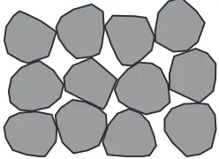
Although simple and relatively computationally inexpensive to model, an assembly of discs is problematic as a rep-resentation of a real soil because it leads to excessive rolling of individual particles. In DEM more realistic shapes are usually achieved by combining multiple discs into clusters. Box2D provides an efficient algorithm for modelling convex polygon-shaped bodies and it was decided to take advantage of this feature in the present study. The particles were modelled as randomly shaped convex dodecagons. Fig. 3 shows an example of the particles used in the simulations. The length to width ratio of particles was set to 1·0 in order to limit the effect of the initial fabric on the results. Particles

were of uniform sizedb, wheredbis defined as a diameter of a

circle bounding the full extent of a given particle.

Simulation accuracy

The accuracy of the simulation can be controlled by adjusting

the time step size,Δt, and the maximum number of velocity

iterations per time step available to the constraint solver,Ni.

Additionally, for given values of Δt and Ni, accuracy is

affected by the ratio of the force experienced by a given particle to its mass. A high ratio will lead to a high tentative velocity, and consequently to large velocity errors that then have to be corrected by the constraint solver (as target velocities will be close to zero in a quasi-static analysis). Therefore, in the biaxial compression test described in this paper the values of confining pressure and density could be selected with a view to maximising accuracy for a given run time, rather than to replicate laboratory test settings (i.e. as this test simply involves an assemblage of rigid particles under zero gravity, these parameters will not affect the physics of this quasi-static simulation).

Sample preparation

The simulation input parameters are given in Table 1. Particles were created simultaneously at a random position

and at a random orientation within a two-dimensional zone

of approximately 50 × 166db; the particles were not allowed

to overlap. The sides of the zone were bounded by tem-porary, rigid, frictionless walls. Once created, the particles were allowed to fall under gravity. After all the particles had come to rest, the top of the sample was levelled, gravity was gradually reduced to zero and the temporary side walls

were removed. The final sample size was 50 × 100db. The

initial sample density was controlled by the particle friction

coefficient (μg) used at the sample generation stage.

The exact shape and drop position for each particle were determined by the random number generator; in order to check repeatability both test setups were run three times with different seeds. The initial void ratios for all specimens are listed in Table 2.

Confining stress

The confining pressure in the horizontal direction was simu-lated by applying forces to the centre of mass of the particles at the perimeter of the specimen. Boundary particles were determined automatically in each time step by casting multi-ple horizontal rays along the height of the specimen. The force applied to a boundary particle was proportional to the

Fig. 3. Polygon-shaped particles used to improve realism

Table 1. Biaxial compression of polygon particle specimens: simulation input parameters

Parameter Value

Soil particles

Coefficient of friction μgorμs Coefficient of restitution 0

Density 5000 kg/m2

Size,db 1·0 m*

Test setup: general properties

Time step size 1/60 s

Number of velocity iterations per time step 100 Number of position iterations per time step 3 Position error correction scaling factor 0·2† Approximate number of particles 5000 Test setup: sample generation stage

μgfor loose sample 0·6

μgfor dense sample 0·2

Gravity 0·1 m/s2

Test setup: shearing stage

μs 0·6

Coefficient of friction of the top cap

and the bottom boundary 1·0

Confining pressure 1 kN/m

Top cap velocity 0·005 m/s

*

For convenience the default length unit in Box2D of metres was used in this study.

†_{Default value in Box2D.}

Table 2. Biaxial compression of polygon particle specimens: void ratios

Seed Loose sampleel Dense sampleed

eled el Initial global average

1 0·311 0·258 0·17

2 0·308 0·259 0·16

3 0·307 0·260 0·15

RVE at 15% axial strain

1 0·296 0·296 0·00

2 0·295 0·290 0·02

number of rays hitting the particle in a given time step. The confining pressure in the vertical direction was

applied by a‘servo-controlled’rigid top cap. The confining

pressure was applied incrementally until the sample was in equilibrium at 1 kN/m. The particle coefficient of friction was then gradually changed to the value used for

shearing (μs).

Biaxial compression

The compression was strain controlled with deviatoric stress applied by the top cap moving vertically at a constant

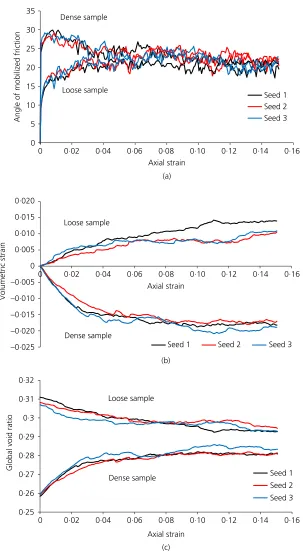
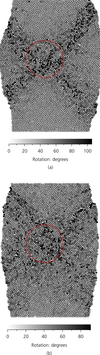
velocity. Fig. 4(a) shows the mobilisation of the angle of friction with the axial strain for both the loose and dense states (three simulations per state). The corresponding evolution of volumetric strain and global void ratio are shown in Figs 4(b) and 4(c), respectively. Figs 5(a) and 5(b) show particle arrangement and accumulated rotation at 15% axial strain of the seed 1 dense and the seed 1 loose samples, respectively.

Overall the results show reasonably good repeatability between simulations. Qualitatively all the dense and the loose samples display behaviour typical of that obtained in laboratory experiments. The loose samples contract and the 0

5 10 15 20 25 30 35

Seed 1 Seed 2 Seed 3 Dense sample

Loose sample

0·25 0·26 0·27 0·28 0·29 0·3 0·31 0·32

0 0·02 0·04 0·06 0·08 0·10 0·12 0·14 0·16

Global void ratio

Axial strain

Seed 1 Seed 2 Seed 3 Loose sample

Dense sample –0·025

–0·020 –0·015 –0·010 –0·005 0 0·005 0·010 0·015 0·020

Volumetric strain

Angle of mobilized friction

Axial strain

(b)

(c) Axial strain

Seed 1 Seed 2 Seed 3 Loose sample

Dense sample

0 0·02 0·04 0·06 0·08 0·10 0·12 0·14 0·16 0 0·02 0·04 0·06 0·08

(a)

0·10 0·12 0·14 0·16

dense samples dilate upon shearing, consistent with critical state behaviour. However, the global average void ratios plotted in Fig. 4(c) do not converge as expected. Figs 5(a) and 5(b) show that in the loose system, shear deformations are spread across most of the sample, whereas in the dense system shearing is localised in distinctive bands, with large

parts of the sample undisturbed by shearing, and having local void ratios largely unchanged from the initial values. In Figs 5(a) and 5(b) a volume element (RVE) considered to be representative of the part of the sample that underwent shearing is indicated by a red circle. Each RVE contained approximately 10% of the sample volume and was posi-tioned in the zone with the highest density of particles having high accumulated rotation. The void ratios in the RVEs of all samples at 15% axial strain are given in Table 2. The results show that parts of the samples that underwent shearing converged, or are very close to convergence, to a consistent critical state void ratio.

The mobilised angle of friction also converges to the

critical state valueϕcrit, of about 21·5°, for both the loose and

the dense states. The dense samples exhibit peak strength behaviour, with a peak angle of friction of about 29°; the peak strength corresponds to the maximum rate of dilation.

Considering that ϕcrit of sands observed in laboratory

experiments is in the range of 32–37° (Bolton, 1986), the

simulated shear strength appears low. However, this can be attributed to the relatively simple soil model used in this study. It is widely accepted that particle angularity and eccentricity have significant influence on the soil shear

strength (Cho et al., 2006) and that the particle size

distribution is also relevant (Morgan, 1999). This means that it is possible to achieve higher shear strength in Box2D by using model properties which are more representative of

that of a real soil. For example, Pytloset al.(2015) observed

a higher value ofϕcrit(29° as opposed to 21·5° found here)

when using particles of a different geometry and non-uniform size.

CONCLUSIONS

A physics engine is a software library used in the film and computer games industries to realistically animate a physical system. Box2D, a widely used open-source rigid body physics engine, has been shown to be capable of accurately simulating disc interaction dynamics. The accuracy achieved was superior to that achieved using the PFC2D and DDAD DEM codes quoted in the literature. It has been demon-strated that Box2D can successfully capture the critical state type response of granular media with particles modelled as randomly shaped polygons. This work suggests that Box2D is a viable alternative to the current two-dimensional DEM tools for modelling particulate media, providing a simple and intuitive physics model.

The simulation method presented here has two potential advantages over a traditional DEM code based on the distinct element method that make it worthy of further investigation. First, physics engines used in computer games are designed to enable fast real-time simulations and this has the potential to translate into corresponding speed benefits for large particulate systems. Second, unlike traditional DEM approaches, the contact model does not appear to require extensive tuning and therefore the soil macro-scale behaviour would only be controlled by particle shape, size distribution and coefficient of friction, all of which can be a direct representation of the physical properties of the soil being modelled.

ACKNOWLEDGEMENT

The authors would like to thank the reviewers for their constructive comments on an earlier version of this manu-script. This work was supported by the Engineering and Physical Sciences Research Council, under grant number EP/l014489/1.

0 20 40 60 80 100

Rotation: degrees (a)

0 20 40

(b)

60 80

Rotation: degrees

REFERENCES

Bender, J., Erleben, K. & Trinkle, J. (2014). Interactive simulation of rigid body dynamics in computer graphics.Comput. Graphics Forum33, No. 1, 246–270.

Bender, J., Erleben, K., Trinkle, J. & Coumans, E. (2012). Interactive simulation of rigid body dynamics in computer graphics. EUROGRAPHICS 2012 State of the Art Reports, Eurographics Association, Cagliari, Sardinia, Italy. See https:// code.google.com/p/bullet/downloads/ (accessed 08/06/2015). Bolton, M. (1986). The strength and dilatancy of sands.

Géotechnique36, No. 1, 65–78.

Catto, E. (2006). Fast and simple physics using sequential impulses. Proceedings of game developer conference. San Jose, CA, USA, see https://code.google.com/p/box2d/downloads/ (accessed 30/03/2015).

Catto, E. (2009). Modeling and solving constraints.Proceedings of game developer conference. San Francisco, CA, USA, see https:// code.google.com/p/box2d/downloads/ (accessed 30/03/2015). Catto, E. (2011).Box2d: A 2d physics engine for games (version

2.2.1), software. See http://box2d.org/.

Catto, E. (2014). Understanding constraints. Proceedings of game developer conference. San Francisco, CA, USA, see http://box2d.org/downloads/ (accessed 30/03/2015).

Cho, G.-C., Dodds, J. & Santamarina, J. C. (2006). Particle shape effects on packing density, stiffness, and strength: natural and crushed sands.J. Geotech. Geoenviron. Engng132, No. 5, 591–602. Coumanns, E. (2012).Bullet physics library (version 2.80), software.

See http://bulletphysics.org/.

Cundall, P. (2001). A discontinuous future for numerical modelling in geomechanics?Proc. Instn Civ. Engrs–Geotech. Engng149, No. 1, 41–47.

Cundall, P. A. & Strack, O. D. (1979). A discrete numerical model for granular assemblies.Géotechnique29, No. 1, 47–65. Erleben, K. (2005).Stable, robust, and versatile multibody dynamics

animation. PhD thesis, Department of Computer Science, University of Copenhagen, Denmark.

Esmaeilzadeh, H., Blem, E., Amant, R. S., Sankaralingam, K. & Burger, D. (2012). Dark silicon and the end of multicore scaling. IEEE Micro32, No. 3, 122–134.

Izadi, E. & Bezuijen, A. (2015). Simulation of granular soil behaviour using the bullet physics library. In Geomechanics from micro to macro (K. Soga, K. Kumar, G. Biscontin & M. Kuo (eds)). pp. 1565–1570. London, UK: Taylor & Francis Group.

Jean, M. (1999). The non-smooth contact dynamics method. Comput. Methods Appl. Mech. Engng177, No. 3, 235–257. Morgan, J. K. (1999). Numerical simulations of granular shear

zones using the distinct element method: 2. effects of particle size distribution and interparticle friction on mechanical behav-ior.J. Geophys. Res.: Solid Earth (1978–2012) 104, No. B2, 2721–2732.

O_’Sullivan, C. (2011). Particle-based discrete element model-ing: geomechanics perspective. Int. J. Geomech. 11, No. 6, 449–464.

O’Sullivan, C. (2015). Advancing geomechanics using dem. In Geomechanics from micro to macro (K. Soga, K. Kumar, G. Biscontin & M. Kuo (eds)). pp. 21–32. London, UK: Taylor & Francis Group.

O’Sullivan, C. & Bray, J. D. (2003). Modified shear spring formulation for discontinuous deformation analysis of particu-late media.J. Engng Mech.129, No. 7, 830–834.

Pytlos, M., Gilbert, M. & Smith, C. (2015). Simulation of granular soil behaviour using physics engines. In Geomechanics from micro to macro (K. Soga, K. Kumar, G. Biscontin & M. Kuo (eds)). pp. 163–168. London, UK: Taylor & Francis Group.

Radjai, F. & Richefeu, V. (2009). Contact dynamics as a nonsmooth discrete element method.Mech. Mater.41, No. 6, 715_–728. Rowe, P. W. (1962). The stress–dilatancy relation for static

equilibrium of an assembly of particles in contact. Proc. R. Soc. London, Ser. A.: Math. Phys. Sci.269, No. 1339, 500–527.

WHAT DO YOU THINK?