Adaptation of short-term plasticity parameters via
error-driven learning may explain the correlation between
activity-dependent synaptic properties, connectivity motifs
and target specificity
Umberto Esposito1, Michele Giugliano1,2,3and Eleni Vasilaki1,2,4*
1
Department Computer Science, University of Sheffield, Sheffield, UK
2Theoretical Neurobiology and Neuroengineering Laboratory, Department Biomedical Sciences, University of Antwerp, Antwerp, Belgium
3Laboratory of Neural Microcircuitry, Brain Mind Institute, Swiss Federal Institute of Technology of Lausanne, École Polytechnique Fédérale de Lausanne, Switzerland
4
INSIGNEO Institute for in Silico Medicine, University of Sheffield, Sheffield, UK
Edited by:
Cristina Savin, Institute of Science and Technology Austria, Austria
Reviewed by:
Rui Ponte Costa, University of Oxford, UK
Alberto Bernacchia, Jacobs University Bremen, Germany
*Correspondence: Eleni Vasilaki, Department Computer Science, University of Sheffield, Regent Court, 211 Portobello Street, S1 4DP Sheffield, UK
e-mail: [email protected]
The anatomical connectivity among neurons has been experimentally found to be largely non-random across brain areas. This means that certain connectivity motifs occur at a higher frequency than would be expected by chance. Of particular interest, short-term synaptic plasticity properties were found to colocalize with specific motifs: an over-expression of bidirectional motifs has been found in neuronal pairs where short-term facilitation dominates synaptic transmission among the neurons, whereas an over-expression of unidirectional motifs has been observed in neuronal pairs where short-term depression dominates. In previous work we found that, given a network with fixed short-term properties, the interaction between short- and long-term plasticity of synaptic transmission is sufficient for the emergence of specific motifs. Here, we introduce an error-driven learning mechanism for short-term plasticity that may explain how such observed correspondences develop from randomly initialized dynamic synapses. By allowing synapses to change their properties, neurons are able to adapt their own activity depending on an error signal. This results in more rich dynamics and also, provided that the learning mechanism is target-specific, leads to specialized groups of synapses projecting onto functionally different targets, qualitatively replicating the experimental results of Wang and collaborators.
Keywords: short-term plasticity, long-term plasticity, learning, rate code, motifs, target-specificity
1. INTRODUCTION
It is the current belief that experiences and memories are regis-tered in long-term stable synaptic changes. Long-term plasticity, and in particular Hebbian learning or Spike-Timing-Dependent-Plasticity (STDP), is a form of unsupervised learning that cap-tures correlations in the neuronal input. Hence, their involvement in, for instance, the development of receptive fields (e.g.,Song et al., 2000; Clopath et al., 2010) or memory and associations is standing knowledge. However, the variety of different long-term plasticity rules (Markram et al., 2011), indicates that the precise synaptic prescriptions of long-term plasticity mechanisms remain unclear.
On the contrary, short-term plasticity (STP) is well-described (Varela et al., 1997; Markram et al., 1998b; Le Be’ and Markram, 2006; Rinaldi et al., 2008; Testa-Silva et al., 2012; Costa et al., 2013; Romani et al., 2013) in the context of specific models (Tsodyks and Markram, 1997; Hennig, 2013; Rotman and Klyachko, 2013). Its role in neuronal computation is assumed to be related to tem-poral processing, see for instance (Natschläger et al., 2001) or
the work by Carvalho and Buonomano (2011), where STP is
demonstrated to enhance the discrimination ability of a single
neuron (i.e., a tempotron, seeGütig and Sompolinsky, 2006), when presented with forward and reverse patterns. Synapses with STP are also optimal estimators of presynaptic membrane potentials (Pfister et al., 2010).
The investigation of the brain wiring diagram known as con-nectomicshas recently made spectacular progress and generated excitement for its perspectives (Seung, 2009). Novel discover-ies in molecular biology (Wickersham et al., 2007; Zhang et al., 2007; Lichtman et al., 2008), neuroanatomical methods (Denk and Horstmann, 2004; Chklovskii et al., 2010), electrophysiol-ogy (Song et al., 2005; Hai et al., 2010; Perin et al., 2011), and imaging (Friston, 2011; Minderer et al., 2012; Wedeen et al., 2012) have pushed forward the technological limits for ultimate access to neuronal connectivity. The comprehension of this level of organization of the brain (Kandell et al., 2008) is pivotal to under-standing the richness of its high-level cognitive, computational and adaptive properties, as well as its dysfunctions.
2011). The occurrence of stereotypical connectivity motifs was experimentally demonstrated and, in some cases, accompanied by physiological information on neuronal and synaptic proper-ties (Song et al., 2005; Wang et al., 2006; Silberberg and Markram, 2007; Perin et al., 2011), on activity-dependent short-term and long-term plasticity (Buonomano and Merzenich, 1998) and rewiring (Chklovskii et al., 2004; Le Be’ and Markram, 2006). Recent experimental findings obtained in young ferret cortices (Wang et al., 2006) indicate that short-term facilitation and depression correlate to specific connectivity motifs: neurons con-nected by synapses exhibiting short-term facilitation form pre-dominantly reciprocal (bidirectional) motifs; neurons connected by synapses exhibiting short-term depression form unidirectional motifs. Interestingly, the same overexpression of connectivity motifs has been observed in another brain area, i.e., the excitatory microcircuitry of the olfactory bulb (Pignatelli, 2009).
Earlier work byVasilaki and Giugliano (2012, 2014)attempted to shed light on this correlation between STP and the observed wiring diagram configuration. They demonstrate that all facilitat-ing or all depressfacilitat-ing networks, upon receivfacilitat-ing the same wave-like stimulation, give rise to the experimentally observed motifs: bidi-rectional for facilitating synapses and unidibidi-rectional for depress-ing synapses. This was explained both in the context of mean field analysis and microscopic simulations as a frequency-dependent effect. This is a simple consequence of the type of input (wave like) and the choice of the STDP triplet rule (Pfister and Gerstner, 2006). Differently from the classical pair rule, the triplet rule dis-plays a frequency-dependent behavior, which can explain some experimental results (Sjöström et al., 2001): at low frequencies the rule reveals the classic STDP and, given a wave-like input, it results in unidirectional connectivity (Clopath et al., 2010; Vasilaki and Giugliano, 2014). At high frequencies, however, it reveals “classic Hebb” behavior: neurons that fire together, wire together. Hence, the low firing network develops unidirectional connectivity, while the high firing network develops bidirectional connectivity; for details see (Vasilaki and Giugliano, 2014). However, the observed synaptic development was not associated to any particular type of learning, but was explored as the emerging structure upon receiv-ing a wave like input: what the network learnedper se in that context was not clear.
With the present work we aim to complement and extend on Vasilaki and Giugliano (2012, 2014). We define a learning model for STP through which a population of neurons can modify its synapses in order to adapt its own activity and then fulfill a given time-varying task. The key idea comes from an optimiza-tion perspective: neurons that are able to modify their synapses, for instance making depressing synapses more and more depress-ing or even turndepress-ing them into facilitatdepress-ing ones, would allow for much more flexibility and efficacy in signal transmission. A simi-lar argument can be found inMarkram et al. (1998a), whereas for earlier but different mechanisms of STP optimization or learn-ing we redirect to Natschläger et al. (2001) andCarvalho and Buonomano (2011).
Then, we construct a typical inverted associative learning problem (Asaad et al., 1998; Fusi et al., 2007; Vasilaki et al., 2009b) where neurons have to learn to respond with high or low frequen-cies, when presented with the same wave-like input signal. We use
this paradigm to show the potential of our model. In particular, not only do we provide an explanation for the correspondence motifs-synaptic properties within the context of learning both STP and STDP (triplet rule) but we also qualitatively capture, for instance, the heterogeneity in synaptic properties observed by Wang et al. (2006).
Moreover, having defined the learning model as a target-specific mechanism, we are able to obtain variability in the short-term profile of synapses innervating functionally different targets. Finally, we show that the learning model can be reduced to a minimal model where only the time constant of recovery from depressionτrecneeds to be learnt in order to obtain neurons firing at high or low frequency. Comparing this finding with the results fromCarvalho and Buonomano (2011), we suggest that differ-ent parameters of the model describing STP might be related to different types of coding.
2. MATERIALS AND METHODS 2.1. SINGLE NEURON MODEL
Each neuron is modeled as inCarvalho and Buonomano (2011): the sub-threshold dynamics of the electrical potentialViof the generic neuroniare described by the equation:
dVi
dt = −gLVi+
N
j=1,j=i
gij(Erev−Vi) , (1)
whereErev=30mV is the reversal potential andgL=0.1μSis the leak conductance - both quantities are equal and fixed for all neurons.giji,j=1,...N is the matrix of conductances and the generic element gij represents the conductance of the synapse going from neuronjto neuroni. Upon arrival of a presynaptic action potential elicited by neuronj, each of the conductancesgij withi=1, . . .N,i=jincreases by a quantitywij, called effec-tive synaptic efficacy, and decays exponentially back to zero with a fixed time constantτg =10ms, equal for all synapses:
dgij
dt = − gij
τg +
f
wijδ
t−tjf, (2)
where tfj is the f-th spike emitted by neuron j. The effective synaptic efficacy depends on both presynaptic and postsynaptic factors:
wij=rijuijAij, (3) whererijanduijare the presynaptic variables representing depres-sion and facilitation in the STP model (see Subsection 2.2) andAij is the postsynaptic variable for the maximum synaptic strength (or absolute efficacy), which represents the maximum synaptic response (see Subsection 2.7). IfVi(t)≥1mV a spike is elicited by neuroniandVi(t+dt) is set to 0 for the nexttref =10ms (refractory period).
2.2. STP MODEL
the degree of depression and facilitation of the synapse connect-ing neuronjto neuroni. The time course ofrijanduijis given by the following kinetic equations (Markram et al., 1998b; Maass and Markram, 2002):
drij
dt =
1−rij
τrecij − N
j=1,j=i
f
rijuijδ
t−tjf (4)
duij
dt =
Uij−uij
τfacilij
+
N
j=1,j=i
f
Uij
1−uij
δt−tjf.(5)
Uij,τrecij andτfacilij are the parameters of the model and they rep-resent, respectively: fraction of resources used by the first action potential, time constant of recovery from depression and time constant of synaptic facilitation. A learning rule for STP has to allow changes to (at least one of) these parameters. At each synapse, the product of rij and uij determines the presynaptic efficacy.
2.3. STDP MODEL
We use the triplet learning rule defined byPfister and Gerstner (2006)with hard bounds: maximum weights can only vary in the interval [Amin,Amax]. In this model, each neuron has two presy-naptic variablesm1,m2and two postsynaptic variableso1,o2. In the absence of any activity, these variables exponentially decay toward zero with different time constants:
τm1
dm1i dt = −m
1
i τm2
dm2i dt = −m
2
i
τo1
do1i dt = −o
1
i τo2
do2i dt = −o
2
i (6)
whereas when the neuron elicits a spike they increase by 1:
m1i →m1i +1 m2i →m2i +1 o1i →o1i +1 oi2→o2i +1.(7)
Then, assuming that neuron i fires a spike, the STDP
implementation of the triplet rule can be written as follows:
ASTDPji = −γo1j (t)A−2 +A−3m2i (t−)
ASTDPij = +γm1j(t)A+2 +A+3o2i (t−) (8)
whereγ is the learning rate,is an infinitesimal time constant to ensure that the values ofm2i ando2i used are the ones right before the update due to the spike of neuroni, andAijis the maximum strength of the connection fromjtoi. Values of STDP ampli-tudes are taken fromPfister and Gerstner (2006)and are listed inTable 1.
In order to setAminwe note that if the maximum weights con-necting the input neurons to a specific output neuron all collapse to zero in the low firing rate regime, then, in the subsequent high firing rate regime, inputs were not able to “wake up” this neu-ron: it remained almost silent all the time. To avoid this, we set
[image:3.595.301.549.75.478.2]Amin=10−3. With such a small value we can still apply the sym-metry measure (Esposito et al., 2014), which assumesAmin=0, see Subsection 2.9, to evaluate the symmetry of the network.
Table 1 | Parameters used in simulations.
Symbol Description Value
N Number of total neurons {40,80}
Nin Number of input neurons {30,60}
Nout Number of output neurons 10
Erev Reversal potential 30 mV
gL Decay constant of neuron potential 0.1μS
τg Decay constant of synaptic conductances 10 ms
Vthr Threshold potential for spike emission 1 mV
tref Refractory period 10 ms
νin Input firing rate 10 Hz
νtarg Output target firing rate {2,20}Hz
τmin
facil Facilitation time constant - minimum value 1 ms τmax
facil Facilitation time constant - maximum value 000 ms τmin
rec Depression time constant - minimum value 100 ms
τmax
rec Depression time constant - maximum value 900 ms
Umin Synaptic utilization - minimum value 0.05
Umax Synaptic utilization - maximum value 0.95
¯
η Fixed learning rate forU,τrec,τfacil 0.1
A+2 Amplitude of maximum weights change - pair term in Long-Term Potentiation
4.6×10⁻³
A+3 Amplitude of maximum weights change - triplet term in Long-Term Potentiation
9.1×10⁻³
A−2 Amplitude of maximum weights change - pair term in Long-Term Depression
3.0×10⁻³
A−3 Amplitude of maximum weights change - triplet term in Long-Term Depression
7.5×10⁻⁹
τm1 Decay constant of presynaptic indicatorm1 16.8 ms
τm2 Decay constant of presynaptic indicatorm2 575 ms
τo1 Decay constant of postsynaptic indicatoro1 33.7 ms
τo2 Decay constant of postsynaptic indicatoro2 47 ms
Amin Lower bound for maximum synaptic weights 0.001
Amax Higher bound for maximum synaptic weights 1
γ Learning rate for STDP and for STP-dependentw {1,2}
dt Discretization time step 1 ms
STDP parameters are as in the nearest-spike triplet-model, described inPfister and Gerstner (2006).
2.4. LEARNING TASK
Neurons are divided into different populations, each of them is required to fire at one of the two target firing rates: 30 Hz (high) or 5 Hz (low). To allow the populations to reach their target rate, both short- and long-term plasticity parameters are adapted via error-driven learning (see Subsection 2.6) and, in addition, the maximum synaptic strength is shaped by the STDP triplet rule (see Subsection 2.3).
2.5. INPUT SIGNAL AND INPUT NEURONS
In all simulations, the input signal is delivered only to a subset of neurons in the network, which we call input neuronsNin. Each of these neurons receives a pulse-like stimulus with a fixed frequency
after another with a fixed time delaytdelayand in a fixed order. We choosetdelay=(νinNin)−1so that neurons that belong to input cyclically receive a stimulus. To further explain this, one may imagine labeling the neurons depending on the order they receive the stimulus, and therefore on the firing order, then have the fir-ing patternN1,N2,N3, . . . ,NNin,N1,N2,N3, . . . ,NNin,N1, . . ., with each pair of adjacent spikes being separated by a time inter-val of tdelay. We can think of the Nin neurons as if they are organized in a ring and the stimulus as a cyclically traveling wave across this ring. To include the effect of noise, a ran-dom Gaussian variable with zero mean and standard deviation equal to 0.1tdelay is added to the firing times. The magnitude of the standard deviation is such that there is no inversion in the firing order. With this construction, the stimulus delivered to input neurons can be thought as generated by an external (not explicitly simulated) population of neurons where each external neuron projects only onto one corresponding input neuron.
Note that, by construction, in the absence of any other signal, the firing pattern of the input neurons reflects that of the stim-ulus. This means that the external signal implicitly fixes a level of minimum activation for theNinneurons: their firing rate can-not be smaller thanνin. Due to this constraint, the input neurons, despite being free to change their parameters according to STP learning rules (see Subsection 2.6), are not totally free to regulate their firing activity, which may prevent them from effectively ful-filling the task. The rest of the neurons, instead, are totally free to adapt their activity and are called output neurons. For these reasons, we read out the interesting quantities only from out-put neurons (we refer to Results and toFigures 1A,4Afor more details on the architecture).
2.6. ERROR-DRIVEN LEARNING RULE FOR STP
The task can be formulated as an optimization problem where neurons regulate their own activity in order to minimize the objective function defined as:
E=
ν
targ− ν
νlim 2
, (9)
where νlim is the maximum allowed frequency due to the
refractory period (νlim=1/tref),νtargis the target firing rate and
νis the mean firing rate across a single population. To calculate firing rates of single neuronsνi we use an exponential moving average with time constantτν=1s:
τνdνi
dt = −νi+ ˆνi (10)
whereνˆiis the current firing rate, which basically reflects if neu-ronihas fired νˆi=1Hz
or not νˆi=0Hz
. The population mean firing rate is therefore:
ν = 1 Npop
Npop
i=1
νi (11)
withNpopbeing the size of the population.
By following a standard procedure, learning rules can be derived from Equation (9) by applying the gradient descent method (Hertz et al., 1991). Since the task is not based on single neurons but it involves an entire population, we use a mean-field approach for the derivation of the learning rules. Therefore, from now on in this section, we switch from the above single neu-ron notation to mean-field variables, by dropping theijindices. It is worth noting that in our formulation the target is achieved not by directly acting on the firing rates, but by tuning the STP parameters, which in turn affects the firing itself. Therefore,ν =
νU, τrec, τfacil
and by using the chain rule we can formally write the following update rule for each parameterp:
p= −ηp∂E
∂p = −ηp
∂E
∂ν
∂ν
∂p =2ηp
νtarg− ν
ν2
lim
∂ν
∂p ,
p=U, τrec, τfacil (12)
whereηpis the learning rate, which in principle could be different for each parameter. The form of the functionνU, τrec, τfacil can be derived with a semi-heuristic procedure, following (Vasilaki and Giugliano, 2014). Whenever possible, for the mean-field variables we use the same symbols as in Vasilaki and Giugliano (2014)for consistency. Thus, we introduce the mean-field variables u, x, U, and A, respectively describing facilita-tion, depression, synaptic utilization and maximum strength. We assume a threshold-linear gain function between input mean currenth and output mean firing rate ν =a[(h−ϑ)]+, for some constantsa, ϑ. We can then write the dynamic mean-field equations for a population of neurons recurrently connected by short-term synapses as follows (Chow et al., 2005):
⎧ ⎪ ⎨ ⎪ ⎩
τh˙= −h+Auxν +Iext
˙ x= 1τ−x
rec −uxν
˙ u= Uτ−u
facil − +U(1−u)ν
(13)
where Iext is the mean external current and τ is a decay-ing constant. By imposdecay-ing equilibrium conditions, h˙= ˙x= ˙
u=0, and combining the resulting equations, we can finally write:
h=F(νh)=
AUν−1+τfacil
ν−2+ ν−1Uτ
facil+ ν−1Uτrec+Uτfacilτrec
+Iext (14)
Now we observe that by taking the limith→ ∞inF(νh)we obtain an upper bound for the maximum allowed firing rate
ν ≤ A
τrec +Iext (for more details see Vasilaki and Giugliano,
2014). We can heuristically turn the above inequality into an equality:
ν = A
τrec+
Iext (15)
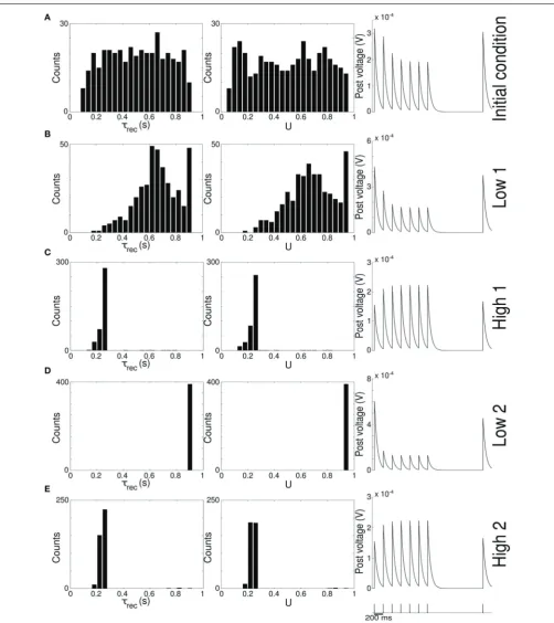
FIGURE 1 | Single population scenario: network architecture and activity, connectivity and STP parameters adaptation in the output population with (U, τrec) learning scheme (Part 1). (A)
Architecture. The learning network (green) is divided into an input region (blue) and an output region (red). Connections (black arrows) are all-to-all and obey both Spike-Timing Dependent Plasticity and rate-dependent Short-Term Plasticity. Input neurons receive an external wave-like stimulus (blue dashed arrows). (B) Mean firing rate of the output population. Shaded area represents standard deviation, horizontal dotted gray lines show the two
target firing rates (high =30 Hz, low =5 Hz) and vertical black arrows mark the onset of the four dynamic phases alternating the target according to the sequence low-high-low-high. (C) Symmetry measure applied on the connectivity of the output population. In accordance to the target, connectivity switches between unidirectionality (low values) and bidirectionality (high values). (D,E) Mean values of the recovery time constant τrec and synaptic utilization U for the synapses projecting onto the output neurons. We observe depression (high values) at low firing rates and facilitation (low values) at high firing rates.
only one of the three parameters appears in Equation (15), we have a single rule forτreconly:
τrec= −2ητrec
νtarg− ν A
ν2
limτrec2
(16)
Then, according to the above derivation, the only parameter that needs to be learnt isτrec. Here we adopt the view (Tsodyks
they apparently play a similar role, we can heuristically take a sim-ilar dependence ofνuponU:ν = UA +Iext, which leads us to a similar learning rule:
U= −2ηUνtarg− ν A
ν2
limU2
(17)
With the same heuristic argument we can also write down a relation involving τfacil. Indeed, it is well-know that facilita-tion/depression corresponds to large/small values ofτfacil, so we can hypothesize a linear relation, also including the dependence on the maximum strength for similarity with the other parame-ters. Thus,ν ∝Aτfacil+Iext, which gives the following learning rule:
τfacil=2ητfacil
νtarg− ν
A
ν2
lim
(18)
Finally, based on the fact thatAturns out to appear in Equation (15), and supported by experimental results showing an inter-action between STP and STDP (Markram et al., 1997; Sjöström et al., 2003), we can also introduce a STP-dependent learning rule for the maximum synaptic strength:
ASTP= −ηA∂E
∂A = −ηA
∂E
∂ν
∂ν
∂A =2ηA
νtarg− ν
1
ν2
limτrec
. (19)
This synaptic modification clearly does not substitute the tradi-tional STDP, since the two rules come from different mechanisms. Rather, we assume they both contribute to maximum weights changes (see Subsection 2.7).
2.7. SINGLE NEURON LEARNING FRAMEWORK: COMBINING STDP AND STP LEARNING MODELS
Equations (16–19) are mean field learning rules for the four parametersτrec,U,τfacil,A. It is straightforward to turn them into single neuron online learning rules. From now on, we return to a single neuron notation. Similarly to STDP, we hypothesize that modifications of STP are triggered by postsynaptic events: every time neuronielicits a spike, its current firing rate is updated as well as the mean population firing rate. Neuronican therefore backwards regulate its incoming synapses, through the following set of equations:
τrecij = −2ητrecij
νtarg− ν Aij
ν2
limτrecij2
(20)
Uij= −2ηUij
νtarg− ν
Aij
ν2
limUij2
(21)
τfacilij =2ητfacilij
νtarg− ν
Aij
ν2
lim
(22)
ASTPij =2ηAij
νtarg− ν
1
ν2
limτrecij
. (23)
The firing event of the neuronialso triggers STDP, according with Equation (8). This contribution sums up with the above STP-dependent change, so as the total modification of the maximum synaptic strength is:
Aij−→Aij+Atotij , Atotij =ASTDPij +ASTPij . (24)
Note that when we converted mean field population equations into single neuron equations we kept the population mean firing rateν, instead of turning it into the single rateνi. This is because the task is defined at a population level. Learning rates of the three STP parameters are chosen to be equal and error-dependent:
ηpij = ¯η
1+νtarg− ν
νlim 2
, p=U, τrec, τfacil, (25)
withη¯=0.1. The learning rate for maximum synaptic strength, instead, is fixed in time and it is the same as the one used for STDP,
ηAij ≡γ.
Now we have four single neuron rules for the STP learning model, plus an equation for STDP and an equation for combin-ing the different rules for the maximum synaptic strength. All these six rules together, Equations (8, 20–24) form a complete learning scheme for each neuron, which is implemented in our simulations. These rules are now local, since their computation takes place separately in each neuron, but receive a global signal encoding for the task performance error.
2.8. INVESTIGATION OF DIFFERENT RULE COMBINATIONS
In the Results section we consider different learning mechanisms: in addition to STDP, that is crucial for the formation of motifs (Vasilaki and Giugliano, 2012, 2014), different combinations of the four STP rules are taken into account while the remaining parameters are kept fixed. At first we allow only two parameters to change:(i)τrec, because Equation (15) implies that for high fre-quencies this is the only critical parameter for adapting the firing rate of the population, and(ii) U, since it was a key parameter adopted in the work inCarvalho and Buonomano (2011). Then, we introduce the STP-dependent rule on the maximum synaptic strength, Equation (23), with the view to observe a more stable learning process. Following this, we also includeτfacilin the learn-ing scheme for a full parameter adaptation (full model) and finally we investigate the minimal number of parameters that needs to be adapted (minimal model), based on Equation (15). Looking for other parameter combinations might not be meaningful, as Equation (15) indicates the key parameters that are involved in changing the mean firing of the population.
2.9. CONNECTIVITY ANALYSIS
To reveal the type of connectivity in the output population, we use a symmetry index defined as a measure of the symmetry of the connectivity matrixW(Esposito et al., 2014):
s=1− 2
N(N−1)−2M
N
i=1
N
j=i+1
Aij−Aji
HereMis the number of instances where bothAijandAjiare zero, i.e., there is no connection between two neurons. Since in our case connections are bounded in the interval10−3,1,M=0 all the time. Equation (26) is able to capture the presence of global non-random structures in a network, returning a value included in [0,1] . Values ofsclose to 1 reflect the presence of a global bidirectional motif, whereas when sapproaches 0, a unidirec-tional motif is emerging. Note that, in order to apply the measure Equation (26), we assume that the lower bound for connections is 0. However, the choice of a small value such as 10−3does not affect the measure.
2.10. DATA SHARING
We provide the scripts that were used to construct the main figures of the paper in the ModelDB database, accession num-ber:169242.
3. RESULTS
3.1. SINGLE POPULATION WITH A TIME-VARYING TASK: A CONTINUUM BETWEEN FACILITATION AND DEPRESSION First, we apply our learning model to a specific task demonstrat-ing how synapses can change their behavior driven by an external feedback signal. The problem we study is simple: a population of neurons is presented with a stimulus and is required to produce a certain output as a response to that stimulus. Once the learning has been successful, for the same input signal the desirable out-put changes. In other words, neurons are trained to respond to a change in the associative paradigm (inverted associative learn-ing problem), that can be due to, for instance, changes in the environmental conditions.
Let us give a concrete example of an inverted associative learn-ing problem, taken from Asaad et al. (1998). In their work, the authors trained monkeys to associate visual stimuli (pic-tures) with delayed saccadic movements, left or right, with associations being reversed from time to time. Monkeys had to go beyond learning a single cue-response association: they are required to learn to associate, on alternate blocks, two cue objects with two different saccades. In other words, after hav-ing learned the relationobject A, go right, andobject B, go left, the associations were reversed such that now they needed to learn
object A, go leftandobject B, go right.
Similar to the (Asaad et al., 1998) experiment, we assume a binary problem, i.e., environmental conditions can change only between two states, and we measure the neurons’ activity in terms of firing rate. This means that neurons are initially asked to fire at some rate and, after learning this task, they are asked to fire at a different rate, while keeping the same input signal all the time. Thus, the problem we defined is a simpler version of the monkey experiment, with only a single input. In order to train the neurons on the current associative paradigm, an external global signal is required, that can be considered as an error signal (see Section Methods 2.6 and 2.7).
3.1.1. Problem description and network architecture
We created a learning network of N=40 conductance-based
integrate-and-fire neurons (see Section Methods 2.1) all to all connected. Synaptic connections are modified by the STDP triplet rule (Pfister and Gerstner, 2006) and STP is implemented by
using the Tsodyks and Markram model (TM model) described inMarkram et al. (1998b); Maass and Markram (2002).
Figure 1Ashows the network architecture, composed by two non-overlapping regions: a blue one with Nin=30 neurons receiving the input signal and aredone withNout=10 neurons from which we read out the quantities of interest. Note that for clarity, only a few neurons (black circles) and connections (black arrows) are drawn. The network is therefore formed by two func-tionally distinct populations, with the input population delivering the stimulus to the output one. Recursive connections are present within each population and across populations, and they are all plastic, in the sense of both long-term and STP. We refer to this architecture as a first or single population scenario.
The input neurons are stimulated one after the other, follow-ing asequential protocol, and approximately with the same rate,
νin=10 Hz. The amplitude of the stimulus is such that input neurons release a spike every time they receive an input (see Section Methods 2.5). This external source can be thought as an additional population of neurons, which we are not simulating here, where each “external” neuron is connected only with a cor-responding neuron in the input population by means of a fixed feedforward connection (blue dashed arrows).
We hypothesize that the whole learning network (greenregion inFigure 1A) is presented with a sequence of two tasks while the stimulus pattern is kept fixed. The tasks are firing low (5 Hz) and firing high (30 Hz) and the sequence islow-high-low-high. Therefore, neurons have to repeatedly learn a new association and forget the previous one in a dynamic context divided in four phases oftph=100s. We refer to them as: low 1, high 1, low 2, high 2. As discussed at the beginning of this section, this pic-ture is inspired by a typical inverted associative learning problem: considering the monkey experiment fromAsaad et al. (1998)as a metaphor, our scenario provides a simplified version, where instead of having two different inputs,object Aandobject B, we have a single input. Indeed, we can think we are presenting the network with onlyobject Aand while doing this we switch the target association between the two states go right and go left, which correspond to our low and high firing rate targets. We call the desirable context-dependent target rate, νtarg. As described in Methods, the difference betweenνtarg and the current firing rate of each population ν is the error signal that, according which our rate-dependent STP causes synapses to adapt their activity.
In all simulations, single neuron parameters
U, τrec, τfacil,w
ij are initially drawn from uniform distri-butions (fori=j), respectively in [0.05,0.95], [100,900]ms, [1,900]ms,10−3,1. Synaptic variables are initialized at their equilibrium values, i.e.,rij=1 anduij=Uij. All the simulations in this subsection useγ =1 for the high rate regime andγ =2 for the low rate regime. Values of the parameters are listed in Table 1.
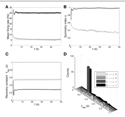
3.1.2. LearningUandτrec
We initially studied the problem with a learning scheme involv-ingUandτreconly, Equations (20, 21), so there is no additional change in maximum synaptic strengths due to STP. Indeed, due
to Equation (15) and (Carvalho and Buonomano, 2011), we
parameters that need to be learnt for adapting the firing rate of a population. The results are displayed inFigures 1B–E, with verti-cal black arrowsmarking the beginning of each of the four phases, and inFigure 2.
Figure 1Bshows the average firing rate of theNout neurons, withshaded areabeing the standard deviation. Target firing rates are show withgray dotted lines. The adaptation to the new target is fast, except during thelow 2phase, when we switch from high to low rate, where an initial fast decrease of the firing rate is followed by a much slower adaptation. Despite the fact that neurons do not reach the target rate during this phase, we observe a monotoni-cally decreasing activity which would eventually stabilize at 5 Hz if we were allowing the simulation to run for longer. The reason for this double slope adaptation will be further discussed now.
Figure 1C shows the evolution of the symmetry index (see Section Methods 2.9). At the beginning, the value reflects the randomness in the connections (the mean value ofsfor a net-work with uniform random connections is indeed0.614, see Esposito et al., 2014), whereas, as learning takes place, we observe the development of unidirectional (low values ofs) and bidirec-tional (high values ofs) motifs, depending on the set target. This can also be formalized by applying thep-value hypothesis test obtained by using mean and variance ofson a completely ran-dom network with uniform distribution of connections (Esposito et al., 2014).P-values are shown inTable 2. We, again, observe rather slow dynamics during thelow 2 phase that, within the fixed simulation time, prevent the system from reaching a clear connectivity configuration. However, the trend ofsclearly shows that the connectivity within the output population is approaching unidirectionality.
Figures 1D,Edepicts the time course of the recovery time con-stantτrecand synaptic utilizationU averaged across the output neurons, withshaded arearepresenting standard deviation. Both parameters oscillate between high values, which correspond to depressing behavior, and low values, that indicate facilitation. Note that the dynamics ofτrec andU is fast in all phases, the third included. This is not surprising since STP is a fast process and leads to fast adaptation of its parameters. As a result, neu-rons’ response to a change in the target rate takes place in a short time. However, during thelow 2phase, synaptic parameters sat-urate before the neurons could fulfill the task, with STDP being the only remaining mechanism through which the output popu-lation can regulate its own activity. This results in a much slower decrease toward the target rate for two reasons:(i)STDP by itself acts on much longer time scales,(ii)switching from high to low rate is the most challenging part of the entire sequence of tasks due to the saturation of the maximum weights in the previous
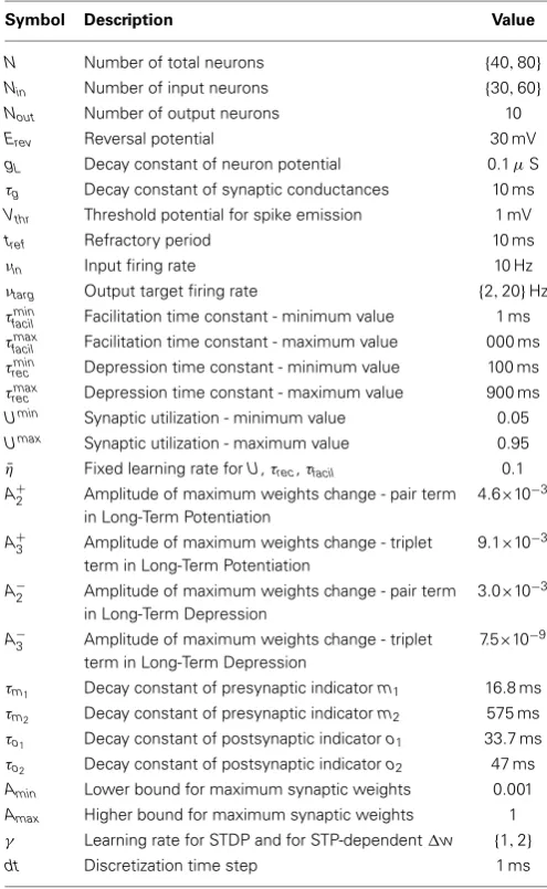
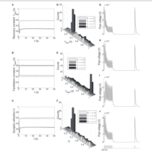
high 1phase, which slows down the process even further. Figure 2 provides additional evidence of the alternation between the two different synaptic behaviors. Plots are orga-nized in five rows, with each row displaying information from a different phase of the simulation. Panel A shows the initial uniform condition, panel B the end oflow 1phase, etc. For each stage, we draw the histograms of recovery time constant (Column 1) and synaptic utilization (Column 2). According to the nar-row standard deviation observed inFigures 1D,E, distributions peak around extreme values, reflecting two different, synaptic
behaviors. Column 3inFigure 2, displaying the single synapse traces obtained with a TM model, demonstrates the correspond-ing behaviors: at the end of the phases where neurons are required to fire low we observe a typical depressing response, whereas at the end of the high rate regimes synapses show a typical facil-itating trace. To generate the traces, we used a 5 Hz signal to stimulate a synapse with a parameters given by the mean val-ues obtained from the corresponding histograms. Note that the synaptic trace for the initial condition, i.e., before learning shapes the parameters, already shows depression, which explains why the distributions ofτrecandUat the end of thelow 1phase are much broader than in the following phases.
Altogether, the four panels(B–E)inFigure 1and the five pan-els(A–E) inFigure 2 show that the properties and activity of the output population oscillate between two states and that the desirable structure is formed depending on the target rate. In particular, we observe that neurons that fire at low frequency turn their synaptic properties into depressing and the connections formed are mostly unidirectional. On the other hand, when the target rate is set at a high frequency, neurons develop facilitating synapses and bidirectional connections.
3.1.3. STP-dependent modification ofAenhances performance Given the speed convergence issue in thelow 1phase, we intro-duced an additional learning mechanism, i.e., the STP-dependent rule forA, Equations (23, 24). Indeed, this mechanism provides an additional way, besides the STDP, for regulating the long-term plastic synapses. In all the other aspects, the model remains as above.
Figure 3shows simulation results, with panels A-D depicting the same quantities as panels B-E inFigure 1(symbols as before). A direct panel-by-panel comparison shows that the results are very similar, meaning that with this new learning configuration the output population also learns to adapt its synaptic properties in order to fulfill the current task, with subsequent motifs for-mation. As expected, due to the additional leaning rule forA, the dynamics are faster: in particular, during thelow 1phase, neurons reach the target rate within the simulation time, and the value of the symmetry measure is much lower than before, confirming the formation of a unidirectional motif; compare withFigures 1C,3B and seeTable 2. Note that the adaptation of the STP parameters is also faster, as they depend on the current value of the maxi-mum synaptic strength. Thus, the STP-dependent modification of
Aimproves the overall performance and introduces an interesting link between STP and STDP.
3.2. TWO POPULATIONS WITH A DIFFERENT TASK: SYNAPTIC DIFFERENTIATION
FIGURE 2 | Single population scenario: STP parameters distribution during adaptation with (U,τrec) learning scheme (Part 2).Different
phases of the dynamics are represented.(A)Initial (uniformly random) condition.(B)End oflow 1phase (target rate is 5 Hz).(C)End ofhigh 1 phase (30 Hz).(D)End oflow 2phase (5 Hz).(E)End ofhigh 2phase (30 Hz).Columns 1, 2Histograms of recovery time constant and synaptic
Table 2 | Symmetry measure andp-value for the single population scenario with{τrec,U}and{τrec,U,A}learning schemes.
Phase (τrec,U) scheme (τrec,U,w) scheme
s p-value s p-value
Low 1(0-500s) 0.36 1.82×10⁻⁹ 0.28 1.13×10⁻¹⁵
High 1(500-1000s) 0.98 5.47×10⁻¹⁹ 0.99 8.73×10⁻²⁰
Low 2(1000-1500s) 0.59 6.47×10⁻¹ 0.41 2.19×10⁻⁶
High 2(1500-2000s) 0.88 1.50×10⁻¹⁰ 0.82 3.63×10⁻⁷
Column 1: the four phases of dynamics with the corresponding simulation time.
Columns 2,3: symmetry measure and p-value for the adaptation ofτrec,U. Values are computed at end of each phase and by considering output
neu-rons only. Columns 4,5 same as columns 2 and 3 except for the adaptation ofτrec,U,A.
learning rules we chose for our model. In particular, we want to test whether our model is able to reproduce existing experimen-tal data, specifically that appearing inTable 1from the paper by Wang et al. (2006).
3.2.1. Network architecture
The new configuration is depicted inFigure 4Aand it is obtained by mirroring the structure of the first scenario and by adding recursive connections between functionally homologous popu-lations. This led to a network of N=80 conductance-based integrate-and-fire neurons, organized in two distinct branches of 40 neurons each, with the first branch required to fire at a high rate (ν=30 Hz) and the second branch at a low rate (ν=5 Hz). Both targets remain fixed throughout the entire simula-tion. Each branch is a replication of the architecture we used previously, i.e., it is formed by an input and an output pop-ulation recursively connected. Thus, the network is formed by four functionally different populations:℘1in,℘in2,℘1out,℘2out, with obvious meaning of symbols. Input populations in both branches receive the stimulus from the same source: a single wave-like signal is delivered to theNinput=60 neurons withν=10 Hz, stimulating one neuron per time (see Section Methods 2.5), first the neurons in ℘in
1 and then the neurons in ℘2in. All connec-tions are plastic following the STDP triplet rule and TM model for STP.
Lateral connections are present between the inputs℘1in, ℘2in and between the outputs ℘1out, ℘2out. To stress that they are functionally different, we drew their initial values from a uniform distribution in10−3,10−1, but, during the evolution, synapses
are allowed to grow up to Amax=1 as any other synapse.
Furthermore, cross connections between different output and input populations, i.e., between℘1in,℘2outand between℘1out,℘2in are absent. The rest of the connections - within each population and across populations belonging to the same branch - are drawn from a uniform distribution in10−3,1 and they are not allowed to exceed this interval during the simulation. STP variables are initialized as in the single population scenario and in all the simulations presented in this subsection we usedγ =2 as the learning rate.
3.2.2. Full model: adaptation ofU,τrec,τfacilandA
We begin by studying the behavior of the full model: all four parameters are modified by our rate-dependent STP, Equations (20–24). Taking into account the modifications of all three STP parameters allows us to make a direct comparison with (Wang et al., 2006). Results are displayed in Figures 4B–C and in Figure 5.
Figures 4B,Cshows the time course of the mean firing rate and symmetry index in both output populations,black linesfor
℘out
1 and light gray linesfor ℘2out. Shaded areasand dark gray
dotted linesrepresent standard deviation and target firing rates. Both populations℘out1 ,℘2outapproach the target rate while devel-oping specific connectivity: as expected, a bidirectional motif emerges in the population firing at the high rate whereas the population firing at the low rate develops mostly unidirectional connections.
Figures 5A–Cshows the time evolution of the three param-eters of the TM model:black lines andgray lines represent the mean value of the synapses projecting from the two output popu-lations℘1out℘2out, respectively onto℘out1 and℘2out. Shaded area is the standard deviation. As expected from the previous sim-ulation, we observe that the two populations develop different synaptic types: high values ofτfaciland low values ofτrecandU, as observed in the population firing at the high rate, suggest a facilitating behavior, whereas values as the one observed in℘2out, characterize depressing synapses. Mean values at the end of the simulation are reported inTable 3rows 1,4. These results show that our model develops target-specific STP and results in good agreement with the data inWang et al. (2006). Indeed, although single values are not identical, the qualitative synaptic behavior is represented: recalling the notation used inWang et al. (2006), two main types of synapses are present. The group projecting from
℘out
1
℘out
2 onto℘out1 can be mapped onto the typeE1 and the group projecting from℘1out℘2outonto℘2outthat can be mapped onto the typeE2.
FollowingWang et al. (2006), we can also refine our classifi-cation, introducing a further distinction within each class. With this purpose, we show inFigures 5D–Fthe distributions ofτrec,
τfacilandU at the end of the simulation within the entire out-put population℘1out℘out2 . For each histogram, data have been divided into four groups, representing the four different subtypes:
℘out
2 to℘2outwithlight gray,℘1outto℘2outwithmedium gray,℘out1 to℘1out withdark gray,℘2out to℘1out withblack. While the dis-tinction between the two synaptic types mapping ontoE1 andE2 is evident, the difference between two subtypes in the same type cannot be easily seen. However, by looking at the mean values of synaptic parameters inTable 3 rows 2, 3, 5, 6 and in partic-ular the ratioτrec/τfacilinTable 3column 5, the distinction into four subtypes becomes more clear. As reported incolumn 7 of Table 3, we can map the synaptic subtypes as follows:E1a corre-sponds to the group℘out1 →℘1out,E1bto℘2out→℘out1 ,E2ato
℘out
2 →℘out2 andE2bto℘1out→℘2out.
FIGURE 3 | Single population scenario: activity, connectivity and STP parameter adaptation in the output population with (U,τrec,A) learning
scheme. (A)Mean firing rate of the output population.Shaded area represents standard deviation,horizontal dotted gray linesshow the two target firing rates (high=30 Hz, low=5 Hz) andvertical black arrowsmark the onset of the four dynamic phases alternating the targets in the sequence low-high-low-high.(B)Symmetry measure applied on the connectivity of the
output population. In accordance with the target rate, connectivity switches between unidirectionality (low values) and bidirectionality (high values).(C,D) Mean values of recovery time constantτrecand synaptic utilizationUfor the synapses projecting onto the output neurons. We observe depression (high values) at low firing rates and facilitation (low values) at high firing rates. Compared toFigure 1, we observe an improvement in the overall performance due to the inclusion of the STP-dependent modification ofA.
Although in Figures 5D–F we present four different
his-tograms for each parameter, we can reason on the overall dis-tribution within the entire output population℘out1 ℘2outas the sample size is the same in all histograms. We can therefore observe that the distribution ofτrecclosely matches that inWang et al.
(2006), whereas the distribution of U reproduces the peak at around 0.25 but is less broad. On the other hand, the distribution ofτfacilis rather different, being totally shifted toward facilitating values in our case. This may be due to the fact thatU is much more peaked around low values. We decided then to discardτfacil from the learning scheme and run a simulation where onlyU,
τrecandAare learnt, as we did for the single population scenario in subsection 3.1.3. We observed that the behavior of the output populations and all the results remain unchanged. We provide an explanation for this in the Discussion.
3.2.3. A minimal model for rate-dependent STP: adaptation ofτrec andA
Finally, we study the minimal model: a model that suffices to obtain the desired behaviors by adapting as few parameters as possible. The choice of the parameters to be learnt is natu-rally suggested by the form of the objective function Equation
(9): τrec and A. Interestingly, this minimal model preserves two key features: (i) both a presynaptic parameter, τrec, and a postsynaptic parameter, A, participate in learning, (ii) STP and STDP are linked to each other through the STP-dependent modification ofA.
InFigure 6we show the results of the minimal model: from A to D, respectively: mean output firing rates, symmetry index,
τrecevolution andτrecdistribution in the four groups of synapses. By comparing these panels with the ones from the full model simulation, we observe that output populations still efficiently fulfill the task while developing the expected connectivity motifs. Also, inTable 4 we report the mean values ofτrec for the four groups of synapses that we identified with the full model: there is still a clear distinction between them. We can therefore conclude that this minimal model is sufficient for qualitatively reproduc-ing the main two types and also the subtypes of Wang et al. (2006).
4. DISCUSSION
FIGURE 4 | Double population scenario: network architecture, activity and connectivity of the output populations with full (U,τrec,τfacil,A)
learning scheme (Part 1). (A)Architecture. The previous network is doubled so that there are now four populations: two input regions (blue) and two output regions℘out
1 ,℘2out(red). The four populations are organized in two branches, one required to fire at high rates (30 Hz) and the second at low rates (5 Hz). Within each branch connections are all to all (black arrows) whereas initially weak connections (gray arrows) are present between the two output populations and between the two input populations. Input neurons receive a wave-like stimulus from outside (blue dashed arrows). All synapses obey both Spike-Timing Dependent Plasticity and rate-dependent Short-Term Plasticity.(B)Mean firing rate of the output populations,black linefor℘out1 , andgray linefor℘
out
2 .Shaded area represents standard deviation andhorizontal dotted gray linesshow the two target firing rates (30 Hz for℘out
1 , 5 Hz for℘out2 ).(C)Symmetry measure applied on the connectivity of the output population. Color legend as in(B). Connectivity evolves differently in the two populations, leading to a bidirectional motif in℘out1 and to a unidirectional motif in℘
out 2 .
introduces two typical synaptic behaviors: depression and facilita-tion. Contrary to long-lasting modifications of maximum synap-tic strengths, for example STDP, existing models of STP do not rely on any learning mechanisms, apart from very few exceptions; see for instance (Carvalho and Buonomano, 2011). Motivated by their work, it is our belief that more efficient dynamics would be possible if synapses were allowed to change their short-term behavior by tuning their own parameters, depending on one or more external controlling factors, for example, their current task. Typically, one asks which is the firing regime for which a cer-tain type of synapse performs better (Barak and Tsodyks, 2007), whereas we are looking at the picture from a reverse perspec-tive: we want to obtain some frequency regime, which is the most efficient way to do it from a synaptic point of view? A similar con-cept can be found inNatschläger et al. (2001), where the authors trained a network with a temporal structured target signal, using optimization techniques.
In our work, we developed a learning scheme for STP, and we obtained, with a semi-rigorous argument, a learning rule for only one of the three parameters of the TM model,τrec. Based on spe-cific experimental results (Tsodyks and Markram, 1997; Markram
et al., 1998b; Thomson, 2000) and data fitting (Chow et al., 2005), we used the conjecture that STP behavior of synapses has the same functional dependence onUandτrec, which allowed us to write a similar rule for the synaptic utilizationU. Interestingly, such learning rules depend on the maximum synaptic strength, and they therefore: (i) provided a natural link between STP and STDP and(ii)allowed us to derive an STP-dependent rule for the maximum synaptic strength, to be added to the STDP contribution.
The interaction between short- and long-term plasticity is largely supported by experimental evidence (Markram et al., 1997), although the exact mechanisms are still unknown. Some results (Markram and Tsodyks, 1996; Sjöström et al., 2003, 2007) suggest that synapses become more/less depressing after long-term potentiation/depression. Our rules incorporate this behavior: long-term potentiation/depression always produces larger/smaller changes in STP parameters. However, whether these modifications bring more facilitation or depression crit-ically depends on whether the population firing rate ν is approaching the target rateνtargfrom above or below. Consider, for example, Equation (16): if νtarg− ν<0, then long-term potentiation will produce a stronger depression, thus reproduc-ing the experimentally observed behavior. In our simulations, this happens to the neurons that are firing at low frequencies. On the other hand, ifνtarg− ν>0, then an increase inAwill make
τrec even smaller, resulting in a less depressing synapse. In our simulations, this happens to the neurons that are firing at high frequencies. A similar argument can be formulated for the induc-tion of long-term depression. We note that several mechanisms have been identified to compete during synaptic transmission, resulting in a more complex and less clear relationship between STP and STDP (Sjöström et al., 2007).
InSjöström et al. (2003, 2007)the authors link the interac-tion between short- and long-term plasticity with the frequency of firing: at high rates, synapses tend to become stronger and more depressing, while at lower frequencies they tend to become weaker and less depressing. Our derivation, instead, suggests the oppo-site: if we rely on the hypothesis that large values ofτreclead to depression and small values to facilitation (Chow et al., 2005), according to Equation (15), facilitating synapses allow neurons to reach higher frequencies. These findings, together with the STDP triplet rule, from the basis of our work: they provide the theoretical basis for the experimentally observed correspondence between facilitation and bidirectionality, and between depression and unidirectionality. The behavior expressed by Equation (15) is experimentally and computationally based on previous work that relates facilitation with high frequency and rate code, and depression with low frequency and temporal code (Fuhrmann et al., 2002; Blackman et al., 2013). This is because, for example, a facilitating synapse may require several spikes to elicit an action potential, meaning that only high frequency stimulation can gen-erate postsynaptic spikes (Matveev and Wang, 2000; Klyachko and Stevens, 2006).
FIGURE 5 | Double population scenario: STP parameters adaptation and final distribution for the output populations with full (U,τrec,τfacil,A)
learning scheme (Part 1). (A–C)Mean values of recovery time constantτrec, facilitation time constantτfaciland synaptic utilizationU.Black linesrepresent mean values across the synapses projecting onto output population 1 from both output populations,℘out
1
℘out
2 →℘1out, whereasgray linesdescribe the synapses projecting onto output population 2 from both output populations,
℘out 1
℘out
2 →℘
out
2 .Shaded areasshow standard deviation. We observe that the two populations develop different synaptic types, facilitating for℘out
1 and
depressing for℘out
2 .(D–F)Corresponding histograms of the three synaptic
parameters at the end of the simulation. For each of them we show four different groups of values, mapping qualitatively to the four subtypes identified byWang et al. (2006), seeTable 3.Light gray:℘out
2 →℘
out
2 (E2a).Medium gray: ℘out
1 →℘
out
2 (E2b).Dark gray:℘ out
1 →℘
out
1 (E1a).Black:℘ out
2 →℘
out 1 (E1b).
(G–J)Single synapse traces obtained with the TM model by using a 12 Hz stimulus. Each panel represents a different subtype of synapses.(G)
℘out
2 →℘out2 .(H)℘out1 →℘out2 .(I)℘out1 →℘out1 .(J)℘2out→℘1out. Synaptic parameters used are the mean values obtained from the distributions drawn in (D–F). A comparison with (Wang et al., 2006) on the basis of the traces only shows that we are able to identify three of the four subtypes.
function has its maximum value, and it is equal to zero for large error. We could have then taken the gradient of the reward function instead, bringing the derived rules into the framework of policy gradient learning methods and reinterpreting the feedback
Table 3 | Types and subtypes of excitatory synapses between the two output populations in the full model{τrec,U, τfacil,A}.
Synaptic groups τrec(ms) τfacil(ms) U τrec/τfacil τrec/τfacilas in Wang Wang’s subtypes
℘out 1
℘out
2 →℘1out 310±11 733±17 0.27±0.01 0.42 0.38 E1
℘out
1 →℘
out
1 260±5 833±13 0.25±0.01 0.31 0.34 E1a
℘out
2 →℘out1 356±19 643±27 0.29±0.01 0.55 0.43 E1b
℘out 2
℘out
1 →℘2out 550±14 440±19 0.55±0.02 1.25 39.47 E2
℘out
2 →℘out2 595±16 436±26 0.61±0.02 1.36 76.88 E2a
℘out
1 →℘out2 510±23 443±28 0.50±0.03 1.15 25.55 E2b
Column 1: synaptic groups. For instance℘out 1
℘out
2 →℘1outincludes all synapses from both output populations,℘out1 and℘out2 , to the output population firing high, ℘out
1 . Columns 2,3,4: mean values of STP parametersτrec, τfacil,U. As inWang et al. (2006), we provide the results in the form mean±s.m.e.. Column 5: ratio between the two time constants,τrec/τfacil, in our simulation. Column 6: for a direct comparison, we provide the values ofτrec/τfacilas inWang et al. (2006). Column 7: mapping of our subtypes onto Wang’s subtypes.
FIGURE 6 | Double population scenario: learning in the output populations with minimal (τrec,A) model. (A)Mean firing rate of the output
populations,black linefor℘out
1 andgray linefor℘2out.Shaded arearepresents standard deviation andhorizontal dotted gray linesshow the two target firing rates (30 Hz for℘out
1 , 5 Hz for℘ out
2 ).(B)Symmetry measure applied on the connectivity of the output population. Color legend as in(B). Connectivity evolves differently in the two populations, leading to a bidirectional motif in
℘out
1 and to a unidirectional motif in℘2out.(C)Mean value of recovery time constantτrec.Black line:℘1out℘2out→℘1out.Gray line:℘1out℘2out→℘2out. We observe that the two populations develop different type of synapses, facilitating for℘out
1 and depressing for℘ out
2 .(D)Corresponding histograms of the recovery time constant at the end of the simulation.Light gray:
℘out
2 →℘2out,medium gray:℘out1 →℘2out,dark gray:℘out1 →℘out1 ,black: ℘out
2 →℘
out
1 . The panels show that the achievement of the tasks and the differentiation of the synapses is still possible with this minimal model.
associated with STDP, and more generally with Hebbian learning, has been extensively studied (Tobler et al., 2005; Izhikevich, 2007; Legenstein et al., 2008).
[image:14.595.302.549.278.383.2]Each of the learning rules we proposed depends, however, on the difference between the target and the actual firing rates, com-puted at the population level. This implies the presence of:(i)a
Table 4 | Types and subtypes of excitatory synapses between the two output populations in the minimal model (τrec,A).
Synaptic groups τrec(ms)
℘out 1
℘out
2 →℘1out 300±9
℘out
1 →℘
out
1 267±6
℘out
2 →℘out1 327±15
℘out 2
℘out
1 →℘2out 524±16
℘out
1 →℘
out
2 486±23
℘out
2 →℘out2 567±22
Symbols are as inTable 3. Similar toWang et al. (2006), we provide the results in the form mean±s.m.e.
single feedback signal encoding the population activity, which is processed outside the population and broadcasted to all neurons;
(ii) an external signal bringing information about the current paradigm, i.e., the target firing rate. Similar toUrbanczik and Senn (2009), we can assume that synapses receive both signals via ambient neurotransmitter concentrations, leading to an on-line plasticity rule.