Robustness Analysis of a Synthetic Translational Resource Allocation Controller

This is a repository copy of

Robustness Analysis of a Synthetic Translational Resource

Allocation Controller

.

White Rose Research Online URL for this paper:

http://eprints.whiterose.ac.uk/134950/

Version: Accepted Version

Article:

Darlington, APS, Kim, J orcid.org/0000-0002-3456-6614 and Bates, DG (2019)

Robustness Analysis of a Synthetic Translational Resource Allocation Controller. IEEE

Control Systems Letters, 3 (2). pp. 266-271. ISSN 2475-1456

https://doi.org/10.1109/LCSYS.2018.2867368

This article is protected by copyright. Personal use of this material is permitted. Permission

from IEEE must be obtained for all other uses, in any current or future media, including

reprinting/republishing this material for advertising or promotional purposes, creating new

collective works, for resale or redistribution to servers or lists, or reuse of any copyrighted

component of this work in other works.

[email protected] https://eprints.whiterose.ac.uk/

Reuse

Items deposited in White Rose Research Online are protected by copyright, with all rights reserved unless indicated otherwise. They may be downloaded and/or printed for private study, or other acts as permitted by national copyright laws. The publisher or other rights holders may allow further reproduction and re-use of the full text version. This is indicated by the licence information on the White Rose Research Online record for the item.

Takedown

If you consider content in White Rose Research Online to be in breach of UK law, please notify us by

Robustness Analysis of a Synthetic Translational Resource Allocation

Controller *

Alexander P.S. Darlington

, Jongrae Kim

and Declan G. Bates

Abstract—Recent research in Synthetic Biology has highlighted the potential of translational resource allocation controllers to improve circuit modularity by dynamically allocating finite cellular resources in response to fluctuating circuit demands. The design of such controllers is complicated by the significant levels of parametric uncertainty that arise in their biological implementations. Tools from robust control, such as µ-analysis, can be used to determine the robustness of controller designs to parametric uncertainty, but require further development to allow their application to biomolecular control systems, which are typically highly non-linear, and contain multiple uncertainties that cannot be represented using the standard linear fractional transformation formalism. Here, we show how an LFT (Linear Fractional Transformation)-free formulation of the µ-analysis problem can be used to analyse and compare the robustness of alternative potential implementations of a translational resource allocation controller that utilises orthogonal ‘circuit-specific’ ribosomes to translate circuit genes. Our results provide useful guidelines for the construction of robust resource allocation circuitry for multiple future biotechnological applications.

I. INTRODUCTION

Synthetic circuits can be created to perform complex com-putations and information processing within cells by assem-bling genetic modules. During the circuit design process it is typically assumed that each module is independent (bar the designed interactions), however, it is now well estab-lished that additional unexpected interactions may emerge as a consequence of the sharing of cellular resources [1]. This breakdown in modularity may not be apparent from gene network models or circuit diagrams during the design phase, and can subsequently lead to loss of functionality or even circuit failure upon implementation in host organisms.

The sharing of translational resources, in the form of free ribosomes, has been implicated as a crucial cause of these non-regulatory interactions [2], [3], since during exponential growth, the pool of ribosomes needed for translation of mRNA (messenger Ribonucleic Acid) into protein is constant [4], and this finite pool of ribosomes is shared across all genes requiring translation. Although similar limitations exist at the transcriptional level, in many settings the resulting effects are small and hence can be neglected [3].

To address the above problems, a prototype translational allocation controller was recently designed and successfully

* This work was supported by the University of Warwick, the EPSRC & BBRSRC Centre for Doctoral Training in Synthetic Biology (grant EP/L016494/1) and the Leverhulme Trust (grant RPG-2017-284)

1 _{APSD and DGB are with the Warwick Integrative Synthetic Biology}

Centre, School of Engineering, University of Warwick, Coventry, CV4 7AL, [email protected]

2 _{JK is with Institute of Design, Robotics & Optimisation, School}

of Mechanical Engineering, University of Leeds, Leeds, LS2 9JT, UK.

[email protected]

Protein synthesis by o-ribosomes

Activated transcription

Inhibitory transcription

Translation

mRNA

Protein

Ribosome

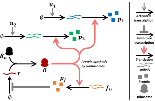
Fig. 1. Genetic architecture of the translational controller. Transcription of the mRNA for proteins p1 and p2 is activated by the inputsu1 and u2

respectively.pf inhibits the transcription of the synthetic ribosomal RNA r. The synthetic RNA converts host-specific ribosomes Rh into

circuit-specific ribosomesRwhich translate all circuit mRNAs and the mRNA of the controller gene into proteins.

implemented experimentally [5]. This controller utilises or-thogonal ‘circuit-specific’ ribosomes which exclusively trans-late circuit genes. By dynamically controlling the production of such orthogonal ribosomes, the effects of resource limita-tions on the gene circuit can be reduced, as circuit-specific translational capacity is increased as demand increases. These o-ribosomes are created by expressing a synthetic rRNA (ri-bosomal RNA)-based component which displaces a core host ribosomal component, changing the machinery’s specificity from host genes to circuit genes [6].

The resource allocation controller regulates the production of this synthetic ribosomal component using negative feed-back, as shown in Figure 1. The size of the circuit-specific o-ribosome pool is controlled by the use of a repressive transcrip-tion factor protein. The protein acts to inhibit the productranscrip-tion of the synthetic ribosomal component by sequestering the latter’s promoter (and so preventing RNA polymerase binding and transcription). The protein is constitutively expressed and translated by the circuit-specific pool. It therefore acts as a sensor of translational demand; as demand increases, the level of this protein falls andvice versa. The inhibitory action of the protein acts to invert this demand signal as it is relayed to the synthetic ribosomal RNA promoter; as protein concentration falls, repression of the promoter through sequestration by the controller protein falls and hence rRNA synthesis increases (and vice versa). Therefore co-option of ribosomes from the host to the circuit-specific pool follows the fluctuating demands made by the circuit.

transla-TABLE I

CIRCUIT AND CONTROLLER PARAMETERS

Description Nominal Units

nσ Number of RNAP per gene 10

σT RNAP concentration 250 nM

nR Number of Ribosomes per mRNA 20

RT Total ribosome concentration 2500 nM

ηi Co-operativity of the input 1

µi Threshold of the input 10 nM

gi,T Geneicopy number 10 nM

kXi Geneipromoter RNAP dissociation constant 200 nM

τi GeneimRNA synthesis rate 320 h-1

kLi GeneimRNA-ribosome dissociation constant 105 nM

γi pitranslation rate 240 h-1

dmi GeneimRNA decay rate 20 h-1

dpi Geneiprotein decay rate 1 h-1

gr,T Synthetic rRNA copy number 500 nM

kXr rRNAPlac(Ptet) promoter dissociation constant 500 (350) nM

τr rRNA transcription rate 190 h-1

dr rRNA decay rate 20 h-1

̺f r:Rhassociation rate 0.9 (nM·h)-1

̺r Rdissociation rate 24.8 h-1

gf,T pfcopy number 10 nM

kXf pfpromoter RNAP dissociation constant 500 nM

τf Geneftranscription rate 320 h-1

kLf GenefmRNA-ribosome dissociation constant 105 nM

γf pftranslation rate 240 h-1

dmf GenefmRNA decay rate 20 h

-1

dpf pfdecay rate 1 h-1

ηf lacI(tetR) co-operativity 4 (2)

µf lacI(tetR) dissociation constant 0.02 (5.6) nM

tional resource allocation controller shown in Figure 1. Due to the underlying biological mechanisms, this model contains many non-linear terms, and as shown below, consideration of uncertainty arising in biological implementations leads to a closed-loop system containing large numbers of real uncertainties (typically kinetic rate constants) that do not enter the linearised system dynamics as polynomial fractions. This poses significant challenges for the application of robustness analysis methods such asµ-analysis, which typically requires the uncertain system to be represented as a linear fractional transformation (LFT), and therefore no formal analysis of the controller’s robustness was attempted in [7].

To address this issue, we here further develop an approach, first proposed in [9], [10], based on combining a randomisation algorithm with a geometric interpretation of the µ-analysis problem. In this approach, the uncertainty is re-defined by a subtraction between the uncertain system and the nominal system. Thus the procedure does not require that the uncertain parameters are actually decoupled from the system (as with LFTs) but only requires the evaluation of the difference between the nominal system and the perturbed system.

II. MODELLING UNCERTAINTY IN A TRANSLATIONAL RESOURCE ALLOCATION CONTROL SYSTEM

Here, we describe the non-linear closed-loop system model, derive its linearisation, and consider the way in which un-certain parameters affect the system. Definitions and nominal values for all parameters in the model are shown in Table I. The non-linear model describes the dynamics of a simple two gene circuit encoding proteins (species p1 and p2) and

the controller system (species pf,r and Rh). The controller consists of the synthetic rRNA species (r), the host ribosomes (Rh) and the protein pf which controls the rate of rRNA synthesis.R represents the free orthogonal ribosome pool.

The dynamics of each circuit protein (pi) follow:

˙

pi=γiRˆci−dpipi (1)

wherep˙i is the derivative ofpi with respect to time and

ˆ

ci= 1

kLi nRτi

dmi

σTxˆi 1 + ˆxi

!

, xˆi=

nσgi,T

kXi

uiηi

uiηi+µi !

(2)

The dynamics of the protein controlling synthetic rRNA syn-thesis is given by:

˙

pf =γfRcˆf−dpfpf

−ηf(nσgr,T−xr−κr)pfηf +ηfµfκr (3)

where

ˆ

cf = 1

kLf nRτf

dmf

σTxˆf 1 + ˆxf

!

and xˆf =

nσgf,T

kXf

(4)

The inhibitory action ofpf at the rRNA promoter is given by

xr= (ˆxrσT)/(1 + ˆxr) (5) ˆ

xr= (nσgr,T/kXr)/[µf/(µf +pf

ηf_{)] (6)} κr= (nσgr,T−xr)[pfηf/(pfηf +µf)] (7)

The dynamics of the synthetic rRNA are given by:

˙

r=τrxr−drr−̺frRh+̺rR (8)

(Note the action ofpf throughxr). The dynamics of the host ribosome pool are given by:

˙

Rh=−̺frRh+̺rR (9)

As the number of ribosomes is fixed, the total number of orthogonal ribosomes (Ro,T) is given by RT − Rh (total ribosomes minus the host ribosomes). These are distributed across all protein encoding circuit and controller genes such that the number of free orthogonal ribosomes is:

R= RT −Rh 1 + ˆcf+ ΣN1 cˆi

(10)

The non-linear model is formed by (1) (repeated once for each circuit genei, here we consider two circuit genes) and (3) to (9). We can define the vectory:= [p1, p2, pf, r, Rh]T. We define y¯ to be the solution to y˙ = 0 and linearise the system around this point.

The linearisation is x˙ =A|y=¯yxwherex=y−y¯andA is the Jacobian. The Jacobian of the system is:

A=      

−_dp

1 0 0 0 −(γ1ˆc1)/K1

0 −_dp

2 0 0 −(γ2ˆc2)/K1

0 0 −_dp

f 0 −(γfˆcf)/K1

0 0 −_K2 −_dr−_̺fR¯_h −_̺fr¯−_̺r/K1

0 0 0 −_̺fR¯_h −_̺fr¯−_̺r/K1

      (11)

whereK1 andK2 expand to:

K1= 1 + ˆcf+ ˆc1+ ˆc2 (12)

K2=

σTηfnσgr,TkXfµfp¯

ηf

f τf ¯

pf(nσgr,Tµf+kXfµf+kXfp¯

ηf

f )2

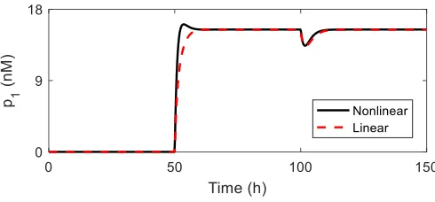
Fig. 2. Simulations of the non-linear closed-loop system and its linearisation for the lacI-based Controller 1. Onlyp1 is shown. Parameters are listed in Table I. Inputs: u1 = u2 = 0 nM while t < 50h. From t > 50 h,

u1= 500nM. Fromt >100h,u2= 500nM.

Figure 2 shows simulations confirming good agreement between the linear and non-linear models for a biological implementation based on the lacI repressor. Upon induction of p2 at100 h, the translational resource allocation controller

successfully rejects the disturbance to p1 caused by resource

mediated coupling.

In general, the Jacobian, A, includes m uncertain parame-ters,δ, which is an element ofRm, i.e.A=A(δ). Allδcan be decoupled from the nominal system, if all theδin the elements of Aappear as polynomial fractions, and the resulting LFT is given by:

˙

x=A(0)x+Bw (14)

z=Cx+Dw (15)

w= ∆z (16)

where A(0) is the nominal system and stable, and ∆ is a diagonal matrix of the uncertain parameters δ. If a system can be represented in this form then the µ-analysis problem becomes a search for the minimum magnitudeδ which gives:

|I−M(jω)∆|= 0 (17)

where | · | is the determinant, j = √−1, ω = [0,∞) and

M(jω) = [jωI − A(0)]−1 _and I _{is the identity matrix}

whose dimension is the same as A. Computationally efficient algorithms exist to findµ-bounds for these systems.

Parametric uncertainty arises in synthetic circuits due to (i) noise in the original measurement (e.g. due to population effects), (ii) changes in transcription/translational kinetics due to new DNA context for genetic ‘parts’ (e.g. [8]) and (iii) fluctuations due to growth conditions/stains (e.g. [2]).

In our model we consider all non-input parameters (i.e. all except u1 andu2) to be uncertain, and model the variability

of a given parameter κ as (1 +δ)κwhere κ is the nominal value and δis the perturbation. Re-considering the linearised model with these added uncertainties shows that it cannot be represented in the necessary form depicted in (14)-(16), as the δ are not polynomial fractions, nor can the uncertain parameters be presented as a diagonal matrix ∆. This is apparent by inspection of the Jacobian in (11), substituting

the disturbancesδx(wherexrepresents the index of the value in the uncertainty vectorδ) yields:

               

−(1 +δ12)dp1 0 0

.. . ...

0 −(1 +δ21)dp2 0

.. . ...

0 0 −(1 +δ34)d_pf M1 M2

0 0 −K2(δ) ... ...

0 0 0 ... ...

                (18)

where M1 and M2 are the fourth and fifth columns of the

uncertain Jacobian:

M1=

   0 0 0

−(1 +δ25)dr−(1 +δ26)̺fR¯h(δ) −(1 +δ26)̺fR¯h(δ)





 (19)

M2=



 

−[(1 +δ10)γ1ˆc1(δ)]/K1(δ)

−[(1 +δ19)γ2ˆc2(δ)]/K1(δ)

−[(1 +δ32)γfˆcf(δ)]/K1(δ)

−(1 +δ26)̺fr¯(δ)−[(1 +δ27)̺r]/K1(δ)

−(1 +δ26)̺f¯r−[(1 +δ27)̺r]/K1(δ)





 (20)

K1(δ)andK2(δ)take the same form as in (13) but with added

perturbations:

K1= 1 + ˆcf(δ) + ˆc1(δ) + ˆc2(δ) (21)

K2=

K2,1K2,2p¯f(δ)(1+δ37)ηf ¯

pf(δ)[K2,3+K2,4+ (1 +δ29)kXfp¯f(δ)

(1+δ37)ηf_]2 (22)

where

ˆ

cf(δ) = 1 (1 +δ31)k_Lf

(1 +δ4)nR(1 +δ30)τf (1 +δ33)d_mf

(1 +δ1)σTxˆf(δ) 1 + ˆxf(δ)

(23)

ˆ

xf(δ) = [(1 +δ3)nσ(1 +δ35)gf,T]/((1 +δ29)k_Xf) (24)

ˆ

c1(δ) =

1 (1 +δ9)kL1

(1 +δ4)nR(1 +δ8)τ1

(1 +δ11)dm1

(1 +δ1)σTxˆ1(δ)

1 + ˆx1(δ)

(25)

ˆ

x1(δ) =

(1 +δ3)nσ(1 +δ13)g1,T (1 +δ7)kX1

u1(1+δ5 )η1

u1(1+δ5 )η1+ (1 +δ6)µ1

(26)

ˆ

c2(δ) =

1 (1 +δ18)kL2

(1 +δ4)nR(1 +δ17)τ2

(1 +δ20)dm2

(1 +δ1)σTxˆ2(δ)

1 + ˆx2(δ)

(27)

ˆ

x2(δ) =

(1 +δ3)nσ(1 +δ22)g2,T (1 +δ16)kX2

u2(1+δ14 )η2

u2(1+δ14 )η2+ (1 +δ15)µ2

(28)

K2,1= (1 +δ1)σT(1 +δ37)ηf(1 +δ3)nσ(1 +δ28)gr,T (29)

K2,2= (1 +δ29)k_Xf(1 +δ36)µf(1 +δ30)τf (30)

K2,3= (1 +δ3)nσ(1 +δ28)gr,T(1 +δ36)µf (31)

K2,4= (1 +δ29)k_Xf(1 +δ36)µf (32)

We also reformulate the steady states of the species¯ywith the uncertainties (e.g.r¯(δ)is the value ofr¯including the necessary perturbations from theδvector).

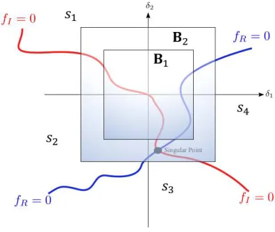
Fig. 3. Interaction of two surfaces and the four possible sign combinations,

sifori= 1, 2, 3and4, inm= 2uncertain space.

III. LFT-FREEµ-ANALYSIS

To implement the LFT-free method we first consider a new representation for the uncertainties:

A∆(δ) :=A(δ)−A(0) (33)

The original uncertain LTI system can be now expressed as

˙

x=A(0)x+A∆(δ)x (34)

Taking the Laplace transform gives:

X(s) =M(s)A∆(δ)X(s) +M(s)x(0) (35)

where X(s) is the Laplace transform x(t), M(s) = [sI− A(0)]−1_{, andx}(0)_{is the initial condition ofx}(t)_.

The robustness problem may be formulated as a search for the δof smallest magnitude which satisfies:

|I−M(jω)A∆(δ)|= 0 (36)

for all frequencies ω ∈ [0,∞). We can now formulate the

µ-analysis problem as follows:

Find the µ (lower bound) and µ¯ (upper bound) such that

µ≤µ(ω)≤µ¯, forω∈[0,∞), where

µ(ω) = (

0, |I−M(jω)A∆(δ)| 6= 0 for allδ,

[dmin(ω)]−1, otherwise,

(37)

where

dmin(ω) = min{d| ∃δ∈Rm,

such that |I−M(jω)A∆(δ)|= 0}

The uncertainty in this problem has no general analytical expression and so standard µ-bound estimation algorithms cannot be applied. However, we can obtain the value for a specificδby evaluating (33). The singularity condition of the determinant is then given by:

fR(δ) =ℜ|I−M(jω)A∆(δ)|= 0 fI(δ) =ℑ|I−M(jω)A∆(δ)|= 0

(38)

where ℜ(·) andℑ(·) denote the real and imaginary parts of a complex number, [9], [10]. These two equalities are (m−

Fig. 4. The number of sign combinations found along the edges ofB1 is

three and thus the size of the box provides aµ-upper bound. On the other hand, the number of sign combinations found along the edges ofB2is four

and thus the size of this box provides aµ-lower bound.

1)-dimensional manifolds on the m-dimensional uncertainty spaceδ. The manifolds divide the uncertainty space into four sections (Figure 3). The exact value ofµis the inverse of the norm of the δ where the two manifolds meet at the singular point (the point highlighted in Figure 3). Any norm could be used in general and the infinity-norm is a frequent choice in

µ-analysis.

Note firstly that, for A∆(0) = 0, i.e. the nominal system, I −M(jω)A∆(δ) is equal to the identity matrix and the

determinant is 1. The real part is 1 and the imaginary part is 0 atδ= 0. Therefore, under the assumption of nominal stability, the manifold where the imaginary part is equal to zero always passes through the origin in the uncertain space, whereas the other manifold, where the real part is equal to zero, always stays away from the origin with a strictly positive distance as depicted in Figure 3. Secondly, the uncertainty space can be divided into four sections:

s1={δ |fR(δ)>0 andfI(δ)>0}

s2={δ |fR(δ)>0 andfI(δ)<0}

s3={δ |fR(δ)<0 andfI(δ)<0}

s4={δ |fR(δ)>0 andfI(δ)<0}

(39)

with each section shown in Figure 3. Now, the number of sign combinations found on boundary boxes of different sizes in the uncertainty space can be counted. In Figure 4, for example, the number of sign combinations on boxes B1 and B2 are

three and four, respectively. Once four sign combinations are found, it can be concluded that the value of µ is inside that box (here boxB2). This leads to the following algorithms for

finding upper and lower bounds onµ(see the Supplementary Material for formal proofs of convergence for these algorithms and MATLAB code for a numerical example):

A. µ-upper bound algorithm

1. Check the sign of the real and imaginary parts of the determinant,I−M A∆, for uniform random samplesδinside

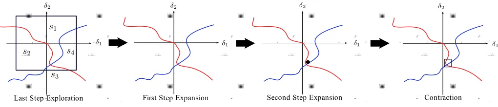
Last Step Exploration First Step Expansion Second Step Expansion Contraction

Fig. 5. µ-lower bound expansion and contraction steps.

B1 or B2 in Figure 4, until either the maximum number of

samples is reached or all four sign combinations are found. 2. If the combinations are not found, increase the size of the hyperbox, otherwise decrease the size of the hyperbox, and repeat. The inverse of the maximum box size which includes samples containing only three sign combinations is the upper bound, e.g. s1,s2 ands4 inB1 in Figure 4.

This algorithm is less conservative than the original algo-rithm presented in [10] as it allows three rather than two sign combinations, as shown in Figure 4.

B. µ-lower bound algorithm

1. Exploration: Check the sign of the real and imaginary parts of the determinant, I −M A∆, for uniform random

samples δ on the faces of a hyperbox centred at the origin in the uncertain space, until either the maximum number of samples is reached or the four sign combinations are found. If the combinations are not found, increase the size of the hyperbox.

2. Expansion & Contraction: In Figure 4 the last sign combination found in B2 from the Exploration step is most

likely to be s3 as this is the smallest area compared to the

others. Checking the sign combinations of random samples inside the box, whose centre is δ corresponds to the sign combination found last in theExplorationstep. The initial box size is the maximum tolerance value. If all sign combinations are not found by the maximum sampling number, the box size is increased. If all sign combinations are found, but the size of the box is greater than the tolerance, move the centre of the box to δ, which is in the middle between two δ’s whose sign combinations were found last and second last. Repeat these steps until some pre-defined maximum number of iterations is reached (in which case the lower bound is zero), or all sign combinations are found in a box centred close to the singular point, where the box size is equal to the given tolerance (in which case the lower bound is the inverse of the distance from the singular point to the origin). A graphical illustration of the procedure is given in Figure 5.

This is a modified and improved version of the µ-lower bound algorithm originally developed in [9], which did not exploit the use of the LFT-free formulation. Specifically, here the expansion step (shown in Figure 5) is improved. Previously, this involved moving the centre of the box to the δ whose sign combination was found last, whereas in the current algorithm the centre of the box is placed in the

middle between twoδ’s whose sign combinations were found last and second last. This avoids occasional problems with the algorithm switching between two regions for many iterations, and significantly improves its convergence properties.

IV. µ-ANALYSIS OF THE TRANSLATIONAL CONTROLLER

We use the above procedure to quantify and compare the stability robustness of four different potential biological implementations of the controller which act to modify key controller design parameters. We analyse three controllers based on the tightly binding LacI repressor, with varyingpf gene copy numbers and RBS strength, and one based on the TetR repressor (Figure 6) which changes dissociation constants and level of cooperativity. We set the uncertainty level for all 36 circuit and controller parameters at ±40% of their nominal values. As shown in Figure 6, our analysis indicates that all potential controller implementations are guaranteed to be stable for this level of uncertainty, since bothµ-bounds are less than 1 at all frequencies. Total computing time to calculate the bounds for each controller was approx. 1 hour (with frequencies calculated in parallel on a 4 core Intel i7 processor with 32 GB RAM). Increasinggf,T (the copy number of the

pf gene) increases robustness, with the upper bound falling from 0.85 to 0.76. DecreasingkLf (i.e. increasing the strength

of the pf ribosome binding site) also increases robustness in comparison to the original case. Changing the repressor used to implement the controller from LacI to another common repressor TetR (hence changing its dissociation constant and co-operativity) also increases the robustness of the controller, (maximumµ-upper bound of 0.76).

Fig. 6. µ-lower and upper bounds for different potential biological implemen-tations scaled by±_{40%. Controller 1 corresponds to thelacI-based design} whose parameters are listed in Table I. Controller 2 corresponds to an increase in gene copy number to gf,T = 500nM. Controller 3 corresponds to an

increase in RBS strength (i.e. a decrease in kL_f = 104 nM). Controller

4 corresponds to atetR-based implementation which changes the following parameterskXr= 350nM,µf = 5.6nM andηf = 2.

V. CONCLUSIONS

In this paper, we have considered the problem of formally quantifying the robustness of resource allocation controllers to parametric uncertainty using µ-analysis. Detailed modelling of resource sharing mechanisms in the closed-loop system revealed that the effects of uncertainty cannot be represented in the form of an LFT, as required by standard µ-analysis tools. We therefore applied an alternative approach, based on a geometric formulation of the µ-analysis problem, that

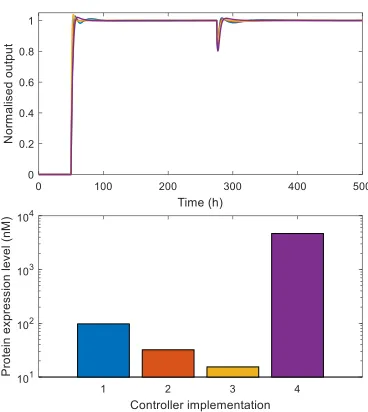
Fig. 7. Simulations of the different biological implementations of the controller using the non-linear model. Levels ofp1normalised by final protein concentration are shown. Inputs:u1=u2= 0nM whilet <50h.t >50h,

u1 = 500nM.t >275h,u2= 500nM.Upper, dynamics normalised by final steady state output.Lower, steady state expression level.

allows the computation of tight bounds onµwithout the need to represent the uncertain closed-loop system in the form of an LFT. This allowed us to evaluate and compare the robustness of alternative potential biological implementations of the controller, thus providing useful guidelines for the construction of robust resource allocation circuitry for multiple future biotechnological applications. The proposed approach should be applicable for analysing the robustness of many kinds of future synthetic biological control circuits.

REFERENCES

[1] Y. Qian, H.-H. Huang, J. Jim´enez, and D. Del Vecchio, “Resource competition shapes the response of genetic circuits,” ACS Synthetic Biology, vol. 6, no. 7, pp. 1263–1272 2017.

[2] F. Ceroni, R. Algar, G.-B. Stan, and T. Ellis, “Quantifying cellular capacity identifies gene expression designs with reduced burden,”Nature Methods, vol. 12, no. 5, pp. 415–423, 2015.

[3] A. Gyorgy, J. I. Jim´enez, J. Yazbek, H.-H. Huang, H. Chung, R. Weiss, and D. Del Vecchio, “Isocost lines describe the cellular economy of genetic circuits,”Biophysical Journal, 109(3), pp.639–646, 2015. [4] M. Scott, C. W. Gunderson, E. M. Mateescu, Z. Zhang, and T. Hwa,

“Interdependence of cell growth and gene expression: origins and consequences.”Science, vol. 330, no. 6007, pp. 1099–1102, 2010. [5] A. P. S. Darlington, J. Kim, J. I. Jimenez, and D. G. Bates, “Dynamic

al-location of orthogonal ribosomes facilitates uncoupling of co-expressed genes,”Nature Communications, vol. 9, no. 695, 2018.

[6] O. Rackham and J. W. Chin, “A network of orthogonal ribosome·_mRNA pairs,”Nature Chemical Biology, vol. 1, no. 3, pp. 159–166, 2005. [7] A. P. S. Darlington, J. Kim, J. I. Jimenez, and D. G. Bates,

“Engineering Translational resource allocation controllers: Mechanistic models, design guidelines and potential biological implementations,” bioXriv Pre-print doi:10.1101/248948.

[8] S. Cardinale and A. P. Arkin, “Contextualizing context for synthetic biology - identifying causes of failure of synthetic biological systems,”

Biotechnology Journal, vol. 7, no. 7, pp. 856–866, 2012.

[9] J. Kim, D. G. Bates, and I. Postlethwaite, “A geometrical formulation of the µ-lower bound problem,”IET Control Theory & Applications, vol. 3, no. 4, pp. 465–472, 2009.