quantum systems and its application to
quantum cascade laser structures
Cite as: AIP Advances 9, 095019 (2019); https://doi.org/10.1063/1.5095246
Submitted: 08 March 2019 . Accepted: 05 September 2019 . Published Online: 13 September 2019
Density matrix superoperator for periodic
quantum systems and its application
to quantum cascade laser structures
Cite as: AIP Advances9, 095019 (2019);doi: 10.1063/1.5095246 Submitted: 8 March 2019•Accepted: 5 September 2019• Published Online: 13 September 2019
Aleksandar Demi ´c,a) Zoran Ikoni ´c,b) Robert W. Kelsall,c) and Dragan Indjind)
AFFILIATIONS
School of Electronic and Electrical Engineering University of Leeds, LS2 9JT Leeds, UK
a)Electronic mail:[email protected] b)Electronic mail:[email protected] c)
Electronic mail:[email protected]
d)
Electronic mail:[email protected]
ABSTRACT
In this work we present a generalization of the Liouvillian superoperator for periodic quantum systems that can be formulated through partitioned Hamiltonians. We formulate a compact algebraic form of the superoperator that allows efficient numerical implementation along with the possibility of further generalization and the inclusion of the system’s boundary effects (i.e. device contacts). We apply this formalism to Quantum Cascade Laser structure where we compare the second nearest and the nearest on approximation, and present the laser dynamics that is independent from the number of states considered.
© 2019 Author(s). All article content, except where otherwise noted, is licensed under a Creative Commons Attribution (CC BY) license (http://creativecommons.org/licenses/by/4.0/).https://doi.org/10.1063/1.5095246., s
I. INTRODUCTION
The Density matrix (DM) formalism was first introduced by J. Von Neumann1–4and its applications span through a variety of fields in Quantum Mechanics. The time evolution of the density matrix is, generally, described by the master equation in Lindblad form5–8and one of the key aspects of this equation is that it results in a nonlinear system of equations, if written in the matrix form. However the system can be linearized by introducing the Liouvil-lian superoperator and the goal of this paper is to present a math-ematical formalism that can generalize and simplify the superop-erator of the systems with high symmetry, in particular periodic quantum systems, such as Quantum Cascade Lasers (QCLs) and graphene.9
QCLs10are powerful semiconductor sources of coherent radi-ation in the mid-infrared (MIR)11 and Terahertz (THz) band12 with potential applications in free-space communications, medical diagnostics, and chemical sensing.13–17These devices use sequential tunnelling and usually comprise a large number of semiconductor heterostructure periods (typically GaAs/AlGaAs for THz QCLs).
The DM model has been successfully applied to QCLs18–34 and it represents a quantum model35that can describe key aspects of the underlying physics while retaining low numerical complex-ity when compared to the more extensive models, such as the Non-Equilibrium-Green Function (NEGF) approach.36–38
The most common applications of the DM model are for sys-tems with a few states, which usually yield analytic expressions.4The Liouvillian superoperator enables the generalization to systems of any size, however, treating periodic systems usually allows elimina-tion of a large number of equaelimina-tions due to the system symmetry, and to our knowledge, compact form of the Liouvillian has not been considered in detail.
dynamical aspects to the model we presented in Ref.33. SectionV presents concluding remarks, and in the Appendix we discuss alge-braic derivations and present the most general formulation of the superoperator for any system that can be partitioned.
II. THEORETICAL MODEL
A. Liouvillian superoperator
The DM formalism describes a quantum system as a statistical ensemble of quantum states through an operator̂ρ= ∣̂ψ⟩⟨̂ψ∣which, provided with the corresponding basis of wavefunctions∣̂ψi⟩, results in a matrix where each elementρijrepresents coherence of statesi andj. The time evolution of the density matrix is then given by the Liouville equation:
dρ
dt = − i ̵
h[H,ρ] (1)
which represents the quantum mechanical analogue of the equa-tion of moequa-tion in the classical systems. It can be further generalized by adding effects that cause decoherence of the system in a form −(dρ
dt)relax. This depends on the problem of interest and we will
discuss these additional terms in the next section.
The formulation in Eq.(1)employs interaction of two oper-ators, and outcome of such interaction is usually referred in the literature as a superoperator. The actual mathematical need for the introduction of the linear superoperator in Eq.(1)arises from the fact that the unknown is a matrix, and that in algebraic sense Eq.(1) is not linear. In mathematics, systems that take the formAXB=Y are linearized asA⊗BTX′
=Y′
where⊗represents the Kronecker tensor product andX′ andY′are vectorised forms of the original matricesXandY, respectively, unpacked row by row in a column vector (for column by column unpacking, the linearization reads AT⊗B). We will keep the notation with an apostrophe’ to refer to these vectorised forms throughout this paper. In our case the com-mutator linearizes in a formL=H⊗I−I⊗HTwhereIis an identity matrix of the same size as the HamiltonianH. The linear operatorL is called Liouvillian superoperator and the linearization of Eq.(1)in the form ddρt′ = −̵hiLρ
′ is a well known formulation of the density
matrix superoperator in the literature.3We also note that if we had Pstates in the basis of wavefunctions of the overall quantum system, the superoperator would be a matrix ofP2×P2size andρ′would be a column vector of lengthP2.
In many practical cases of interest, we need to deal with Hamil-tonians which are partitioned in the block form, and may have high degree of symmetry, especially in cases which deal with periodic systems, where the wavefunction basis can be taken only on one period and not from the entire quantum system. InAppendix Bwe show a simplified algebraic way of forming a superoperator if the Hamiltonian and the corresponding density matrix are partitioned in block form without any particular symmetry. In further consider-ations we will focus on Hamiltonians with high level of symmetry, often employed in tight binding39 and the nearest first or second neighbour approximations.
Consider a periodic quantum system in which we can for-mulate a wavefunction basis from one period and describe the
Hamiltonian of that period as H0 and its corresponding density
matrix asρ0. Note that if the wavefunction basis hasNstates,H0
andρ0areN×Nmatrices. The HamiltonianH0can interact with
the adjacent periods (as depicted inFig. 1) given by block Hamil-tonians H1, H2, . . .HM (to the right) and H−1, H−2, . . . H−M (to the left) which have the corresponding block density matri-ces ρ±1, ρ±2, . . . ρ±M, where M is the number of neighbours that central (H0) period has in either direction. Take a system
consisting of Qperiods (Q≥2M + 1). The Hamiltonian of the entire system can then be written as (2M + 1)-diagonal block matrix of Q × Q block size. In order to apply periodic bound-ary conditions,Q→ ∞andQ×Q, (2M + 1) – diagonalHand
ρ need to be substituted into the Liouville equation. This yields (4M + 1) – diagonal block matrix from the commutator term in (1). This matrix will be equal to the derivative of the density matrix (timesi̵h) and it is clear that there will be some “extra” equations that equal to zero block matrices in the overall density matrix. This occurs due to the algebraic properties of banded matrices. Generally, product ofS– diagonal matrix withT– diagonal matrix is aS+T −1 – diagonal matrix. In our case, if bothHandρare (2M+ 1) – diagonal, the result of their commutator will be a (4M+ 1)– diagonal matrix, and there will be 2Mequations that target zero blocks in the density matrix. We can therefore group equations that Eq.(1)yields into two groups:
Group 1:
ih̵dρk dt =
M ∑ j=0
[H(k−j)sgn(k),ρj],
k= −M, . . .,M,k≠0
ih̵dρ0 dt =
M ∑ j=−M
[H−j,ρj],k=0
(2)
Group 2:
0= M ∑ j=k−M
[Hk−j,ρj],k=M+ 1, . . ., 2M
0= −M ∑ j=k+M
[Hk−j,ρj],k= −2M, . . ., −M−1
(3)
Group 1 has (2M+ 1) block equations, while in group 2 there are 2M additional equations which contain the same unknown density matrix blocks as group 1.
[image:3.594.333.529.559.664.2]The equations in Eq.(3)are the consequence of the duplication of information in the system. We assumed the form of the result-ing density matrix in advance, and therefore forced the system to yield (2M+ 1) equations in Eq.(2). The reason why additional 2M equations emerged is that even though we are forcing the system to have no terms for interaction with (M+ 1)−thneighbour, the included neighbours (2Mof them) still give their contribution to the nextM+Mneighbours and therefore we end up with additional 2Mequations. They originate from the duplication of information from initial symmetry of the Hamiltonian and therefore can be discarded.
The number of neighbours that need to be included in the sys-tem depends on the underlying physics of the syssys-tem. It is also pos-sible to include more density matrix blocks then the number of par-titions in the Hamiltonian. However this is only relevant in strongly coupled systems and in systems where the dissipator term may coherently couple periods that are not coupled by the corresponding Hamiltonian block.
Let us consider a system with the second neighbour approx-imation given by the Hamiltonian and the corresponding density matrix:
H= ⎛ ⎜⎜ ⎜⎜ ⎜ ⎝
H0 H1 H2 0 0
H−1 H0 H1 H2 0
H−2 H−1 H0 H1 H2 0 H−2 H−1 H0 H1 0 0 H−2 H−1 H0 ⎞ ⎟⎟ ⎟⎟ ⎟ ⎠
(4)
and
ρ=
⎛ ⎜⎜ ⎜⎜ ⎜ ⎝
ρ0 ρ1 ρ2 0 0
ρ−1 ρ0 ρ1 ρ2 0
ρ−2 ρ−1 ρ0 ρ1 ρ2
0 ρ−2 ρ−1 ρ0 ρ1 0 0 ρ−2 ρ−1 ρ0 ⎞ ⎟⎟ ⎟⎟ ⎟ ⎠
(5)
Let us apply general expressions in Eq.(2)and neglect Eq.(3), forM= 2 which corresponds to the Hamiltonian and the density matrix given by Eqs.(4)and(5):
i̵h ⎛ ⎜⎜ ⎜⎜ ⎜ ⎝
ρ2 ρ1 ρ0 ρ−1
ρ−2
⎞ ⎟⎟ ⎟⎟ ⎟ ⎠ =
⎛ ⎜⎜ ⎜⎜ ⎜ ⎝
[H0,ρ2]+[H1,ρ1]+[H2,ρ0]
[H−1,ρ2]+[H0,ρ1]+[H1,ρ0]+[H2,ρ−1]
[H−2,ρ2]+[H−1,ρ1]+[H0,ρ0]+[H1,ρ−1]+[H2,ρ−2] [H−2,ρ1]+[H−1,ρ0]+[H0,ρ−1]+[H1,ρ−2]
[H−2,ρ0]+[H−1,ρ−1]+[H0,ρ−2]
⎞ ⎟⎟ ⎟⎟ ⎟ ⎠ (6) Formulating the system of equations in Eq.(6)can be done intuitively: for a given blockρi, equation for that block will consist of all combinations of the Hamiltonian and the density matrix blocks whose indices add toi, provided that the blocks are labelled as in this work.
The primary goal of this work is to simplify Eq. (6) (and Eq.(2)) and provide linear superoperator that can be easily numeri-cally implemented. Equation(6)represents a system of commutator equations where we can define sub-Liouvillian operators which lin-earize each commutator asLi= (Hi⊗I−I⊗HiT)ρ′i,i= −M, . . .M. This then turns Eq.(6)into a linear system which can be written as i̵hdρdt′′ =LQρ′′, whereLQis a (2M+ 1)– diagonal block matrix whose
block elements areLiand it has a similar form as the original block form of the Hamiltonian. The unknowns will represent vectorised forms of the corresponding density matrix blocks, labelled asρ′
i, and we can pack these vectorised vectors in reverse orderi=M,. . .−M into one vector, labelled asρ′′. It is interesting that we can form lin-ear operator for system in Eq.(6)directly from the Hamiltonian by using Khatri-Rao type of matrix product (definition and derivation is given in theAppendix A) denoted by symbol⊠.
Equation(6)linearizes as:
ih̵dρ ′′
dt = (H⊠I N UQ−I
N UQ⊠H
.T)
ρ′′
(7)
whereIUNQis a block matrix partitioned in the same way as the Hamil-tonian, where each block is an identity matrix. Note that the second term in Eq.(7)is “dot” transpose operation which transposes only the partitions within the Hamiltonian, not the Hamiltonian itself. The important advantage of Eq.(7)is its mathematical simplicity and the similarity to the general form of density matrix superopera-tor, since the only difference is in the type of algebraic product (and INUQ matrix and the “dot” transpose operation). This formulation is general for periodic quantum systems where the Hamiltonian and the corresponding density matrix can be partitioned in block form (it applies to Eq.(2)as well).
The main advantage of the formulation in Eq. (7)is that it neatly applies periodic boundary conditions and linearizes the sys-tem in the compact algebraic form. An additional difference from the Liouvillian superoperatorL=H⊗I−I⊗HTis that the super-operator in Eq.(7)packs the unknowns of the system differently and requires the formulation of the system with partitioned Hamilto-nian. Generally, superopetaor for any partitioned Hamiltonian can be formed by using Khatri-Rao product and this is further explained inAppendix B.
The linearization in Eq.(7)uses the Hamiltonian of (2M+ 1) ×(2M+ 1) block size, however once Eq.(7)is solved, it is incor-rect to use such Hamiltonian and the corresponding density matrix for finding the expectation values of operators. The expectation value of any operatorÔin DM formalism can be found as Tr(Oˆρˆ). Trace operation for the partitioned matrix results in a sum of traces of each submatrix, and the productOρ needs to be dound as a limit value when Q → ∞ with an infinite Q × Q, (2M + 1) – diagonal density matrix and the Hamiltonian as discussed in Ref.33in order to ensure the implementation of periodic boundary conditions.
B. Dissipator
Liouville equation(1)describes only the interactions included in the Hamiltonian, however, it is quite common to model some interactions separately by adding phenomenological relaxation terms that damp the equation of motion in the form−(ρτ)relaxor, in a more detailed form−γmn(ρmn−ρ(mneq)), m,n=1, 2,. . .,N, whereγmn are decay rates that damp density matrix termsρmnto their equilib-rium valueρ(eq)
mn , where4ρ eq
mn=0,m≠n. Furthermore, the state pop-ulations (described by the diagonal elements of the density matrix) decay can be also introduced in the form∑En>Em
ρnn
τmn − ∑En<Em ρmm τnm and it appliesγmn = 12(τ1
m −
1
τn)+γ col
decay rates of populations out of levelsmandn, whileγcolmnare the dephasing rates due to the processes (i.e. elastic collisions) that do not affect the state populations, and influence only the phase, these rates are often referred to as proper dephasing rates.4We will refer to all these additional terms in Liouville equation as a dissipator D = −(ρτ)relax of the system; this term follows the symme-try of the Hamiltonian described in the previous subsection, but does not follow a neat algebraic formulation as Eq. (7), even though these terms originate from various interaction Hamil-tonians that could have been included in the total Hamilto-nian H. This term is linear and we can transform it as D →D′′
ρ′′
, however the form ofD′′
can be derived by mathemat-ical induction and it depends on the system considered. In the Appendix C we show how D′′ is derived for QCLs.25,26,33 Equa-tion (1) now acquires an additional termD and Eq. (7)can be written as:
i̵hdρ ′′
dt = (H⊠I N UQ−I
N UQ⊠H
.T −i̵hD′′
)ρ′′
(8)
The reason why D is often excluded from H is because of possible simplifications and physical interpretation of the quantum system under consideration. The Hamiltonian of the system usu-ally consists of several different interaction Hamiltonians that are of interest, however some of them can be considered as perturba-tions and their effect can then be handled by perturbation theory (i.e using Fermi’s golden rule). For example, in laser systems, the rates τmn can be directly expressed via Fermi’s golden rule, and
τm would simply represent state lifetimes. It is important to note that Dmust not break the positivity of the density matrix since the main requirement for a physical solution of Eq. (1) is that
ρ is a positive semi-definite matrix which ensures that all diago-nal elements of the density matrix are positive (which must phys-ically be satisfied). This condition will be satisfied if various scat-tering processes are included inDin Lindblad5form, and Fermi’s golden rule satisfies this condition. Note that carious forms of dissipators can be found in the literature9,30–32 that may also be applied.
C. Dipole approximation
The density matrix formalism is capable of describing optical macroscopic effects of the quantum system along with the effects of external electrical perturbation.
We can assume that the Hamiltonian can be split asH=Hfree +VwhereHfreeis the Hamiltonian of the unperturbed system, and Vis the energy of interaction. The dipole approximation physically models the system as a dipole antenna that will resonate at a specific transition frequency, in this case the energy difference of the levels, and assumes that the interaction energy can be written asV=−μA, whereμ=−eris the electric dipole moment operator4andA(r,t) is the optical electric field.
The most common implementation of the DM formal-ism describes Hfree as a diagonal tight binding matrix (filled with the corresponding energy states Em) and the substitution into the general Liouvillian yields a system of equations in the form:4
dρmn
dt = −iωmnρmn− i ̵
h∑ν(Vmνρνn−ρmνVνn) −γmnρmn, ωmn=Em−̵En
h , m≠n dρnn
dt = − i ̵
h∑ν(Vnνρνn−ρnνVνn) + ∑
Em>En
ρmm
τnm − ∑Em<En
ρnn
τmn
(9)
This equation is actually a closed form of the Liouvillian (L = H ⊗ I − I ⊗ HT + D), where H = Hfree + V and it repre-sents the most common DM formulation4 that is often combined with Maxwell equations. The formulation we presented in Eq.(8) is not equal to the one in Eq.(9). It is somewhat valid to claim that Eq. (8)can be derived from Eq. (9), but it is important to point that the Hamiltonian is different, because it includes inter-actions between the periods and not just the tight-binding Hamil-tonian. Additionally, the order in which both systems of equations are written is different. In Eq.(9)the density matrixρis unpacked row–wise, and the first two terms simply correspond to the alge-braic transformation of the Kronecker product (L = H ⊗ I − I ⊗HT) and periodic boundary conditions are not applied. In Eq.(8) the density matrix was partitioned in blocks as in Eq. (5) and the overall system stores the unknowns by unpacking each block row–wise. For example, in Eq.(6)the overall density matrix first unpacked blockρ2intoN×Ncolumn vector, thenρ1,ρ0. . ., and then joined them into one 5N2column vector which is referred to as ρ′′ in Eq. (7). This somewhat cumbersome repacking in Eq.(8)resolved the problem of deciding which equations in the periodic system can be ignored, how to properly set the periodic boundary conditions and, most importantly, offered the conve-nience in physical interpretation of the system that is described by a partitioned Hamiltonian and the corresponding density matrix.
Furthermore, the approach we present in Eqs.(4,5)can be fur-ther generalized, in order to include the finiteness of system consid-ered (i.e. contacts of the laser structure), which is one of the main advantages of the more general models.36
D. Non-rotating wave approximation
In most cases of interest the optical electric fieldAhas a phys-ically expected form which can greatly simplify the DM model. Generally, A(r, t) should be obtained from Maxwell equations coupled to the DM model via polarization, which is given as
literature, in particular for two-level systems.4 Another common approach treats Eq. (9)by rotating-wave approximation (RWA), however for compact usage in Eq. (8) we will focus on a more general approximation from which RWA was originally derived. Assume that the optical electric field has a general plane-wave form:
A(r,t) = ∑ k
(Ak(r,t)e
iβr−iωkt+A
k(r,t)e
iβr+iωkt+c.c)
A(t) = ∑ k
(Ak(t)e−iωkt+Ak(t)eiωkt+c.c) (10)
where βis the propagation constant. Without loss of generality, we will assume that the optical field has only the time depen-dence, as given by the second equation in Eq.(10). Both of these expressions are used in treatment of DM and Maxwell equa-tions, but the second form can be taken in cases where individ-ual quantum systems are much smaller them the wavelemgth of light.
Non-rotating wave approximation (NRWA) assumes that the system’s response will have identical harmonic form, while RWA discards some terms based on the underlying physics of the sys-tem. Note that implementing the RWA is actually more complicated because we would need to manually select which terms of the den-sity matrix would be allowed to oscillate at +wand which at−w, depending on the energy states that correspond to the particular density matrix elements. NRWA does increase the numerical com-plexity, however it significantly simplifies further formulation of the model.
The drive terms in differential equations(8,9)have a harmonic form due to Eq.(10), and it would appear natural to assume that the solution will follow this structure, i.e.ρ(t) = ∑kρ+k(t)e
iωkt+
ρ−
k(t)e−iωkt. However, this is possible in some special cases when the underlying physics allows it. The generalization of the system in Eq.(8)is far from trivial.
Interestingly, the generalization of the effect of Eq.(10)on DM formulation in Eq.(8)is possible when only one frequency com-ponent is considered, and it can be expressed by a simple algebraic formulation.
To illustrate that, we considerH=Hdc+Hace−iωt+Haceiωtand
ρ=ρdc+ρac−e−iωt+ρac+eiωt, where each term is partitioned and has the (2M+ 1) diagonal form as in Eqs.(4,5). Therefore, each blockHj andρjhas three harmonic terms:Hj=Hdcj +Hjace−iωt+Hjaceiωtand
ρk=ρdck +ρ ac− k e
−iωt+
ρack+e
iωt. Consider the equations resulting from the commutator ofHjandρk:
e−iωt
: [Hjdc,ρ ac− k ]+[H
ac j ,ρ
dc k] e0: [Hjac,ρac
+
k ]+[Hdcj ,ρkdc]+[Hjac,ρac − k ] eiωt: [Hjac,ρkdc]+[Hjdc,ρac
+ k ]
(11)
Each commutator in Eq.(11)can be linearized with the cor-responding sub-Liouvillian, and we will only have two of them: Ldcj = Hdcj ⊗I−I⊗Hdc
T
j ,Lacj =Hacj ⊗I−I⊗Hac T
j and the linear form of Eq.(11)is:
⎛ ⎜⎜ ⎝
Ldcj Lacj 0 Laj+ Ldcj Lacj
0 Lacj Ldcj ⎞ ⎟⎟ ⎠ ⎛ ⎜⎜ ⎝
ρ′ac− k
ρ′dc k
ρ′ac+ k ⎞ ⎟⎟ ⎠ ≡⎛⎜⎜ ⎝ ⎛ ⎜⎜ ⎝
Hjdc Hjac 0 Hacj Hjdc Hjac
0 Hjac Hjdc ⎞ ⎟⎟ ⎠⊠ ⎛ ⎜ ⎝
I I I I I I I I I ⎞ ⎟ ⎠− ⎛ ⎜ ⎝
I I I I I I I I I ⎞ ⎟ ⎠
⊠⎛⎜⎜ ⎝
HjdcT Hac T
j 0
HjacT Hdc T j Hac
T j 0 HjacT Hdc
T j ⎞ ⎟⎟ ⎠ ⎞ ⎟⎟ ⎠ ⎛ ⎜⎜ ⎝
ρ′ac− k
ρ′dc k
ρ′ac+ k
⎞ ⎟⎟
⎠ (12)
The consequence of Eq. (12)is that it affects each equation in Eqs.(2,3), and it breaks each of them into three equations. This causes the system size to increase three times, however the approach we presented in Eq. (8)needs to be just slightly re-modified. In Eq.(12)we can notice that linearization of Eq.(11)can be written in a similar Khatri-Rao notation as used in Eq.(8). We need to apply Eq.(12)to each equation in Eqs(2,3), however we can notice that the structure of Eq.(12)is tridiagonal and we can transform the initial Hamiltonian by defining an expansion rule for non-rotating wave approximation (NRWA) in the form:
HjNRWA→ ⎛ ⎜⎜ ⎝
Hdcj Hjac 0 Hacj Hjdc Hjac
0 Hjac Hjdc ⎞ ⎟⎟ ⎠
(13)
If Eq.(13)is applied to each block of our initial Hamiltonian, the expanded Hamiltonian enlarges 3 times, but the formulation of Eq.(8)is still correct and slightly modified by addingNRWA super-script in each term in Eq.(8), and also adding a term which is a consequence of the time derivative:
ih̵dρ ′′NRWA
dt = (H NRWA⊠
IUNQNRWA−I NNRWA UQ ⊠H
NRWA.T
−i̵hD′′NRWA
+h̵ωΩNRWA)ρ′′NRWA
(14)
NRWAexpansion affects Eq.(8)as follows:
● HNRWA is a 3Q × 3Q Hamiltonian obtained by applying Eq.(13)on each block whereQ= 2M+ 1. Depending on the problem, some blocks may have only some of the frequency terms and this can simplify the problem of interest. ● IUNQNRWA is enlarged 3 times and represents 3Q×3Qmatrix
filled with identity matrices only in positions where the cor-responding Hamiltonian has non-zero blocks. For algebraic convenience, we could also defineIUNQNRWA as block matrix with 9Q2 submatrix identity blocks ofN ×N size, which has direct algebraic formulation from a unity matrixUas IUNQNRWA = U3Q×3Q⊗IN×N. Note that the system in Eq.(8) is banded, and appropriate numerical algorithms can be applied, in contrast to the system in Eq.(9)whose sparse properties are generally broken by the dissipator.
● ρ′′NRWA is a column vector of 3QN2 size, where the first 3N2 elements correspond to stacked vectorised forms of
ρ′ac− k ,ρ
′dc k ,ρ
′ac+
k , k = −M,. . .,Mrespectively, the next 3N
elements correspond to the stacked (in the same order) vec-torised forms that correspond to the next block (M− 1), and so on until all blocks are stored (M,M−1,. . ., 0,. . ., −M+ 1,−M).
● The dissipatorD′′NRWA
usually follows the rule in Eq.(13)and needs to comply with the order of storage of the unknown
ρ′′NRWA. As discussed above, the dissipator of the system depends on the system under study, and therefore its lin-earization and incorporation into the system cannot be defined generally.
● Frequency terms populate the main diagonal of the system, and this is formulated by ΩNRWA. These terms originate from the time derivative in Eq.(14). The algebraic formulation is ΩNRWA = (I2M+1×2M+1⊗G3×3) ⊗IN2×N2 whereGis 3×3 diagonal matrix with entries−1, 0, 1 on the main diagonal. ΩNRWAcan have different mathematical formulations (i.e. IN2×N2 =IN×N⊗IN×Nand various properties of Kronecker product can be used).
Note that the generalization presented so far is only valid for one frequency in Eq.(10). The expansion rule in Eq.(13)can clearly be generalized further if we wanted to include integer multiples of frequencyω. Generally, if we includeFmultiples ofω, the expansion rule in Eq.(13)will then be (2F+ 1)– diagonal (2F+ 1)×(2F+ 1) matrix.
The difficulty for further generalization lies in frequency inter-actions. For example, consider a case where we have two frequency components in Eq.(10),ω1 and ω2. The potential terms are ω1,
ω2,ω1−ω2,ω1+ω2, 2ω1, 2ω2which in NRWA expansion would expand the system up to 12 times, however, depending on the values ofω1andω2and the state energies, some terms may be neglected due to the underlying physics. A good example can be found in Ref.26, where three different frequencies were used for the study of nonlinear effects in QCLs.
In general, any linear system of commutators can be formulated through Khatri-Rao product, and different expansion rules would be needed, depending on the problem of interest.
E. Boundary conditions
Boundary conditions represent the crucial part of the system formulation. In this work we focused on periodic systems described by the banded partitioned Hamiltonian, but the effects of device boundaries will generally appear at all four corners of the Hamil-tonian and therefore break its banded structure. A vast literature is available for boundary conditions of banded matrices40,41 and one of the main advantages of the formulation in this work is that one can include the effects of device contacts, similarly to NEGF methods.36Expectation value of any operatorÔin DM for-malism can be found as Tr(Oˆˆρ). For infinite periodic systemsQ → ∞, and the common approach is to find the limit value of Tr(Oˆρˆ)as in Ref.33, however the result will strongly depend on the chosen boundary conditions, which depend on the problem considered.
III. QUANTUM CASCADE LASER
The derivation in the previous section is general for any peri-odic system and the differences in implementation of the model
lie in the specific forms of the coupling off-diagonal Hamilto-nian blocks and the dissipator. In Refs. 24, 26, and33 we pre-sented one of the simplest nearest neighbour DM implementa-tion that is, in essence, a generalizaimplementa-tion of approach used in Ref. 22. The simplicity of the model comes from the fact that blocksH1 andH−1 which describe the interaction between
adja-cent periods, only have the dc term which consists of Rabi cou-pling strengths given in Ref.42. Note that this approximation is ambiguous for QCL structures since formulation in Ref. 42 con-siders tunnelling coupling rate of a two well system. This may be circumvented by using generalized scattering approach32,34 which also offers generalization of the dissipator beyond the Fermi-golden rule. We will focus on the simpler model and formulate it with Khatri-Rao notation introduced in Eq. (8)and also con-sider the dynamic effects by coupling the model with Maxwell wave equation.
Consider a 3×3 tridiagonal Hamiltonian and the correspond-ing tridiagonal density matrix and the dissipator:
H=⎛⎜ ⎝
H0 H1 0
H−1 H0 H1
0 H−1 H0 ⎞ ⎟
⎠, Υ=eKL ⎛ ⎜ ⎝
I 0 0 0 0 0 0 0 −I
⎞ ⎟ ⎠
ρ=⎛⎜
⎝
ρ0 ρ1 0
ρ−1 ρ0 ρ1
0 ρ−1 ρ0 ⎞ ⎟ ⎠, D=
⎛ ⎜ ⎝
D0 D1 0
D−1 D0 D1 0 D−1 D0 ⎞ ⎟ ⎠
(15)
whereH0is anN×Nmatrix involving itsdcand twoacterms in
the formH0=Hdc +Haceiwt+Hace−iwt.Hdc is the tight-binding
Hamiltonian of one QCL period, which has the main diagonal filled with bound state energies. Matrix Υ describes the effect of the applied biasKand it will slightly influence Eq.(14). The dissipator blocks can all be expressed in the form ρj
τ, and this was reviewed in Ref.33. Interestingly the linearization of these blocks satisfies D′
1=D′−1, more details are given in the Appendix.H ac=eZA
1(t),
whereZis the dipole matrix that corresponds to the single period basis wavefunctions andA1(t) is the optical electric field at radiation
frequencyω.
In Ref. 33we performed steady–state analysis by taking A1
= const and ran a minimization algorithm that varied A1 until
the gain of the device was clamped to the loss due to the satura-tion effect. In this work, we couple the DM model with Maxwell wave equation in order to explore the dynamics of the system. Wave equation can be implemented through travelling wave29 approach or standing wave approach which correspond to the forms in Eq. (10), respectively. In this work we will couple the DM model with the time-dependent-only wave equation which is derived when Maxwell’s equation is approximated with stand-ing waves and we will assume that only one mode in the struc-ture is lasing. Additionally, we will apply slow-varying envelope approximation which is common in laser considerations43 and which turns the wave equation into the first order differential equation.
and then translated to the neighbouring periods, while the effect of the biasKover the period lengthLwould only be noticeable in the Hamiltonian blocks as the energy shift of±eKL. Note that this approximation allows the density matrix in Eq.(15)to have equal diagonal blocks, even though its Hamiltonian broke that symmetry. This will have a significant influence on the derivation of the output parameters.
Generally, the addition of the effect of bias influences Eqs.(2,3) by the addition of the term keKLH0ρk, however substitution in Eq.(15)does not change significantly; the termeKLΥ⊠IUNQshould be added in Eq.(8), its NRWA expansion iseKLΥ→eKLΥNRWA=eKLΥ ⊗I3N×3Nwhich needs to be added in Eq.(14), as is further discussed in theAppendix C. The system of equations that Liouville’s equation yields is:
i̵hd dt ⎛ ⎜ ⎝
ρ1 ρ0 ρ−1
⎞ ⎟ ⎠=
⎛ ⎜ ⎝
[H0,ρ1]+[H1,ρ0]+eKLρ1−ihD̵ 1
[H−1,ρ1]+[H0,ρ0]+[H1,ρ−1] −i̵hD0 [H−1,ρ0]+[H0,ρ−1] −eKLρ−1−ihD̵ −1
⎞ ⎟ ⎠
dA1
dt = −
γ
2A1−i w 2ϵ0n2P
(16)
whereγ= cnαLrepresents the total lossαLmultiplied by the group velocity,nis the refractive index andPis the expectation value of the polarization operator. The system under study is represented by an infinite periodic matrix and the form in Eq. (16) focuses on minimal number of equations that need to be solved, however the expected values of the operators need to be derived through usage of infinitely sized banded matrices, as discussed in Ref.33. In our case, the current density operator ˆJ = ien2D
̵
hL [Hˆ, ˆz]has the expectation value j = ien2D
̵
hL Tr(Z([H1,ρ−1]+[H0,ρ0]+[H−1,ρ1])) + Tr(L(H1ρ−1−ρ1H−1)), and the polarization operator ˆP= −e
n2D L ˆz has the expectation valueP= −en2D
L Tr(Zρ
+
0)wheren2Dis the sheet electron density andZis the dipole matrix that corresponds to the central period basis.
The linearization of the DM part of Eq.(16)is given by Eq.(14) (with addition of +eKLΥNRWAρNRWA′′ term) and numerical imple-mentation is straightforward after the Khatri-Rao formulation is introduced. Full matrix form of all terms in Eq.(14)is given in the Appendix C, together with discussion on the linearization of the dis-sipator part. Note that the DM part of the system in Eq.(16)has threeN×Nblocks of the density matrix, and NRWA expands the system three times, which, after the linearization, has 9N2 differ-ential equations. For the steady–state analysis we can set the time derivatives in Eq. (14) to zero, and the system would be linear and homogeneous. For the study of dynamics, the system is non-linear, however the system is of the first order and various ordi-nary differential equations numerical procedures are available in numerical packages. Normalization condition of the density matrix requires that its trace has unity value. This property only affects the blocks that directly correspond to the basis (Trρdc0 =1) and we
can replace one of the equations in the 9N2system with this con-dition in order to solve the system most efficiently or introduce a substitute that one of the elements is one minus all the others. Note that it is not arbitrary which equation is replaced. Only an equation that contains diagonal elements of the blockρ0 can be replaced.
The algorithm, runs self–self–consistent method for solving Schroedinger-Poisson equation under equithermal subband approx-imation33 withA1 = 1Vm−1 (very low optical interaction) which
yields the highest possible value of the optical gain. If that value is larger then the total loss, the system then uses the steady–state wave-function basis obtained forA1= 1V m−1and couples it with the wave
equation as in Eq.(16).
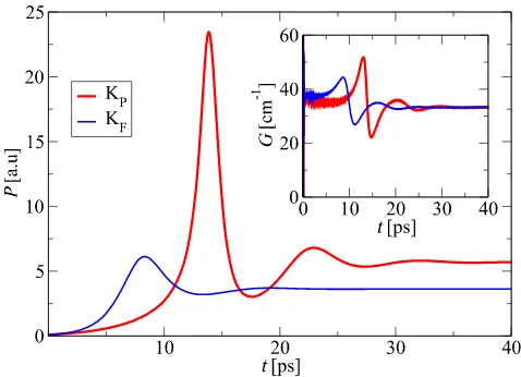
Figure 2shows the dynamic behaviour of 2THz QCL struc-ture33 with layer structure: 5.0/14.4/1.0/11.8/1.0/14.4/2.4/14.4/
2.413.2/3.0/12.4/3.2/12.0/4.4/12.6nm, Al0.1Ga0.9As barriers are
shown in bold, and wells doped to 1.3 1016cm3are underlined. The initial condition for Eq.(16)was set at steady–state solution when optical fieldA1= 103Vm−1. This was done in order to account for
the spontaneous emission in the device. Eq.(16)was solved by using Runge-Kutta-Cash-Karp solver within ODEINT numerical package in C++.
Physically,Fig. 2illustrates the essential property of QCL struc-tures. The relaxation oscillations are barely present as the sys-tem reaches the steady–state much faster then its round trip time (≈60ps), even at the peak power. This dynamic behavior is inde-pendent on the number of states considered, and it can sustain a system with any number of states, in contrast to the common Max-Bloch approaches. In this case, we included complex interactions between twelve states per QCL period. Numerical implementation of the model was made straightforward due to the compact form of the superoperator, Eq.(14), and apart from the tunneling strengths, input for the presented DM model is identical as in RE approach,33 and the main difference is in the mathematical aspect of the system construction.
Note that further numerical simplification is possible if we sep-arate real and imaginary parts of the equations in Eq.(16)and use Hermitian symmetry of the system. Additionally, it may be pos-sible to determine the Jacobian of Eq. (16), use the steady–state point value forA1=constas stationary point and solve the system
[image:8.594.308.547.474.647.2]through eigenvector and eigenvalue approach which may yield faster numerical results.
IV. THE SECOND NEAREST NEIGHBOUR INTERACTION
The nearest neighbour interaction is valid for QCL devices due to the fact that we expect a rapid decay of wavefunctions inside the injection barriers, which makes the interaction of the first and the
third period very weak. Here we consider a simple two–well periodic structure whose wavefunctions extend across three periods, which requires including higher order Hamiltonian and the corresponding density matrix blocks, labelled asH±2andρ±2. The matrix form of the Hamiltonian, density matrix and dissipator have similar form as in Eq.(15), but they are now pentadiagonal matrices, where each matrix has additional super- and sub-diagonal containing block H±2,ρ±2andD±2. The system of equations that Liouville’s equation yields is:
ih̵d dt ⎛ ⎜⎜ ⎜⎜ ⎜ ⎝
ρ2 ρ1 ρ0 ρ−1 ρ−2 ⎞ ⎟⎟ ⎟⎟ ⎟ ⎠ =
⎛ ⎜⎜ ⎜⎜ ⎜ ⎝
[H0,ρ2]+[H1,ρ1]+[H2,ρ0]+ 2eKLρ2−i̵hD2
[H−1,ρ2]+[H0,ρ1]+[H1,ρ0]+[H2,ρ−1]+eKLρ1−i̵hD1 [H−2,ρ2]+[H−1,ρ1]+[H0,ρ0]+[H1,ρ−1]+[H2,ρ−2] −i̵hD0 [H−2,ρ1]+[H−1,ρ0]+[H0,ρ−1]+[H1,ρ−2] −eKLρ−1−i̵hD−1
[H−1,ρ−1]+[H−2,ρ0]+[H0,ρ−2] −2eKLρ−2−i̵hD−2
⎞ ⎟⎟ ⎟⎟ ⎟ ⎠
(17)
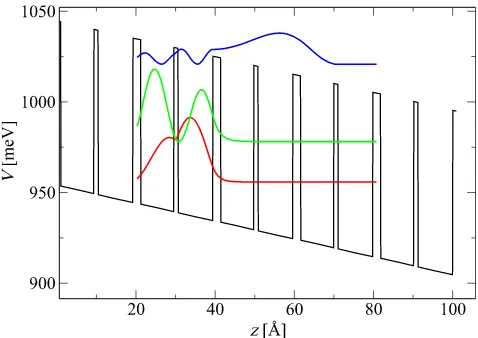
This equation is then linearized as Eq.(14)(with the addition of the term due to the applied electric field). As an example, consider a GaAs/Al0.1Ga0.9As two well periodic structure that has three states,
their wavefunctions extending even into the second neighbour peri-ods (Fig. 3), and therefore solving system in Eq.(17)is necessary. The calculated current density dependence on the applied electric field is shown inFig. 4.
In Figure 4 we can notice that the second nearest neigh-bour approximation did improve the initial result. Note how-ever, that numerical complexity of pentadiagonal model requires solving 15N2 equations when NRWA is employed. This
struc-ture is not a QCL device, but rather an exemplary strucstruc-ture where including the second nearest neighbour interaction is nec-essary. In Table I we focused on a range of bias values where
FIG. 3. Band diagram and wavefunction plot (one period only) for the exem-plar structure. The layer thicknesses, starting from the leftmost barrier are
20/84/10/88Å,Al0.1Ga0.9Asbarriers are shown in bold and the well doped to 1.3×1016cm−3is underlined.
the model difference is most notable inFig. 4. We calculated the overlap integrals of central period wavefunctions across the first neighbouring Fi = ∫F|ψi|2dz and the second neighbouring Si = ∫S|ψi|2dz period. The third wavefunction is strongly coupled in both periods which can also be detected in Fig. 3, and in this bias range, there is also a strong coupling of all three wave-functions in the first neighbouring period. Outlining the neces-sity for the second neighbour approximation is nominally not straightforward. One of the wavefunctions may strongly couple with the second neighbour, however it might not have a signif-icant influence on the transport. The values in Table I give a rough estimate of the effect. We can additionally illustrate opti-cal field effects by investigating absorption saturation, displayed inFig. 5.
[image:9.594.47.286.475.644.2] [image:9.594.310.548.479.646.2]TABLE I. Overlap integrals of wavefunctions |i⟩across the first (Fi) and the second (Si) neighbour period for different values of applied electric biasK(in kV/cm) for a structure inFig. 3
K 4.5 5 5.5 6
F1 0.61 0.62 0.63 0.64
F2 0.41 0.40 0.39 0.39
F3 0.43 0.36 0.29 0.24
S1 1.16⋅10−5 1.25⋅10−5 1.35⋅10−5 1.46⋅10−5
S2 9.92⋅10−5 10.65⋅10−5 11.45⋅10−5 12.34⋅10−5
S3 0.31 0.38 0.44 0.48
FIG. 5. Absorption coefficient dependence on frequency for different values of optical electric field, obtained within the second nearest neighbour approximation. Inset shows the comparison between the nearest (dashed lines) and the second nearest (solid lines) approximation where the absorption coefficients for different values of the optical electric field are displaced for better visibility.
FIG. 6. Current density versus applied electric field obtained by a tridiagonal den-sity matrix33 and pentadiagonal density matrix for QCL structure. Inset shows optical power dependence on current.
InFigure 5we can observe how absorption coefficient gets satu-rated with the increase of optical electric field. Note that here we are not coupling the DM model with Maxwell equation as in the previ-ous considerations, but rather directly changing optical electric field value within the Hamiltonian. Similarly toFig. 4there is a difference in results depending on number of neighbours considered in the DM model, shown in the inset.
Implementing the second nearest neighbour approximation for QCL device uses identical expressions as Eq. (17) and compari-son between the first and the second nearest neighbour approx-imations for QCL structure considered in Ref. 33 is presented inFig. 6.
Figure 6shows nearly identical results as33 and confirms the expectation that expanding the model does not affect the results sig-nificantly. All other results (for material gain and optical power) presented in Ref.33are identical as well.
V. CONCLUSION
We presented a generalization of the Liouvillian for periodic quantum systems that can be represented by (2M + 1)–diagonal partitioned Hamiltonian and the corresponding density matrix. We showed that Khatri-Rao product for the system of commu-tator equations can be applied directly to the initial form of the Hamiltonian, and that it can be written with a similar algebraic notation as the commonly known Liouvillian of non-partitioned Hamiltonian.
InAppendix Awe give further generalization for partitioned approaches which can be applied to a variety of quantum systems. Our formulation allows intuitive physical interpretation of the equa-tions in the system and it can extend the DM model to include the effects of the device contacts, which should make this model competitive with more complex models, such as NEGF approach. We illustrated how NRWA affects the periodic system and dis-cussed key approximations that are commonly introduced in the DM formalism.
We applied our model to an exemplary periodic structure and QCL structure considered in our previous work, where we illustrated that number of partitions in the density matrix and the Hamiltonian depends on localization and span of wavefunc-tions over neighbouring periods. We showed that, when applied to a QCL structure, the superoperator given in Eq.(14) requires nearly identical input and algorithm approach as rate equa-tion models, and the only difference lies in algebra needed for model construction. Note that the sparse-banded nature of the equations that this model yields also enables efficient numerical optimization.
We analyzed the absorption saturation with optical field on periodic exemplary structure and presented dynamical response of the bound to continuum THz QCL structure with twelve states considered. The model can be further developed to investigate dynamical behavior of QCLs.
ACKNOWLEDGMENTS
[image:10.594.48.286.480.653.2]APPENDIX A: ALGEBRAIC SIMPLIFICATION FOR PERIODIC PARTITIONED SYSTEMS
Kronecker tensor product is a well known type of product in algebra44 and for matricesAand B,A⊗Bcreates a block matrix where a block inij–thplace is given asaijB. Kronecker product with the identity matrixIm×mhas a very intuitive form, when performed from the left asIm×m⊗A, the resulting matrix is block diagonal with Ablocks on the main diagonal; when performed from the right asA ×Ithe resulting matrix takes every element inAand multiplies it by identity matrix which visually looks like every element inAwas diagonally stretched. One of the great advantages of the Kronecker product is that it enables linearization of the system. The system in the formAXB=Ycan be linearized as (A⊗BT)X′=Y′for row–wise vectorisation ofXandY.
Khatri-Rao product45–47is defined as a “dot” product of par-titioned matrices, where the “dot” is the Kronecker product, how-ever alternative definitions exist in the literature48 and we will focus on the definition as in Refs. 49 and 50, which requires A andBto be partitioned in the similar form. The Khatri Rao prod-uct would then behave as originally stated. This prodprod-uct is useful, as we have shown in this work, to describe linear systems given by Kronecker products. We made significant algebraic simplifica-tions which allow efficient numerical implementation along with the intuitive physical interpretation of equations given in the block form.
Let us linearize each commutator in Eq. (6) as Li = (Hi ⊗I− I ⊗HTi)ρ′i and separate the terms that multiply the unknowns from the left and from the right into two separate groups as:
ih̵ ⎛ ⎜⎜ ⎜⎜ ⎜⎜ ⎜ ⎝ ρ′ 2 ρ′ 1 ρ′ 0 ρ′ −1 ρ′ −2 ⎞ ⎟⎟ ⎟⎟ ⎟⎟ ⎟ ⎠ = ⎛ ⎜⎜ ⎜⎜ ⎜⎜ ⎜ ⎝
H0⊗Iρ′2+H1⊗Iρ′1+H2⊗Iρ′0
H−1⊗Iρ ′
2+H0⊗Iρ′1+H1⊗Iρ′0+H2⊗Iρ′−1 H−2⊗Iρ
′
2+H−1⊗Iρ ′
1+H0⊗Iρ′0+H1⊗Iρ′−1+H2⊗Iρ ′ −2 H−2⊗Iρ
′
1+H−1⊗Iρ ′
0+H0⊗Iρ′−1+H1⊗Iρ ′ −2 H−2⊗Iρ′0+H−1⊗Iρ′−1+H0⊗Iρ′−2
⎞ ⎟⎟ ⎟⎟ ⎟⎟ ⎟ ⎠ − ⎛ ⎜⎜ ⎜⎜ ⎜⎜ ⎜⎜ ⎝
I⊗HT0ρ′2+I⊗H1Tρ′1+I⊗HT2ρ′0
I⊗HT−1ρ ′
2+I⊗H0Tρ′1+I⊗H1Tρ′0+I⊗H2Tρ′−1 I⊗HT−2ρ
′
2+I⊗H−T1ρ ′
1+I⊗H0ρ′0+I⊗H1Tρ′−1+I⊗H2ρ ′ −2 I⊗HT−2ρ′1+I⊗H−T1ρ′0+I⊗H0Tρ′−1+I⊗H1Tρ′−2
I⊗HT−2ρ ′
0+I⊗H−T1ρ ′
−1+I⊗H T
0 ρ′−2
⎞ ⎟⎟ ⎟⎟ ⎟⎟ ⎟⎟ ⎠ = ⎛ ⎜⎜ ⎜⎜ ⎜⎜ ⎜ ⎝
H0⊗I H1⊗I H2⊗I 0 0
H−1⊗I H0⊗I H1⊗I H2⊗I 0 H−2⊗I H−1⊗I H0⊗I H1⊗I H2⊗I
0 H−2⊗I H−1⊗I H0⊗I H1⊗I 0 0 H−2⊗I H−1⊗I H0⊗I ⎞ ⎟⎟ ⎟⎟ ⎟⎟ ⎟ ⎠ ⎛ ⎜⎜ ⎜⎜ ⎜⎜ ⎜ ⎝ ρ′ 2 ρ′ 1 ρ′ 0 ρ′ −1 ρ′ −2 ⎞ ⎟⎟ ⎟⎟ ⎟⎟ ⎟ ⎠ − ⎛ ⎜⎜ ⎜⎜ ⎜⎜ ⎜⎜ ⎝
I⊗H0T I⊗HT1 I⊗H2T 0 0
I⊗H−T1 I⊗H T
0 I⊗H1TI I⊗HT2 0
I⊗H−T2 I⊗H T
−1I I⊗H T
0 I⊗HT1 I⊗HT2
0 I⊗H−T2I I⊗H−T1 I⊗HT0 I⊗HT1
0 0 I⊗HT−2 I⊗H T −1 I⊗H
T 0 ⎞ ⎟⎟ ⎟⎟ ⎟⎟ ⎟⎟ ⎠ ⎛ ⎜⎜ ⎜⎜ ⎜⎜ ⎜ ⎝ ρ′ 2 ρ′ 1 ρ′ 0 ρ′ −1 ρ′ −2 ⎞ ⎟⎟ ⎟⎟ ⎟⎟ ⎟ ⎠ (A1)
The first term on the right in Eq.(A1) results in a block matrix that has the same form as the Hamiltonian in Eq.(4), where each block goes through Kronecker⊗product with the identity matrix I. Similarly, the second term results in a matrix that has a form of block transpose (or “dot” transpose) of the Hamiltonian, where blocks go through Kronecker tensor product withIfrom the left. It is clear that we can extract the Hamiltonian and its block transpose in Eq.(A1)and let them undergo “dot” product like operation with a (2M+ 1) diagonal matrix filled with identity matrices, where “dot” would represent Kronecker product. This type of product is known as Khatri-Rao product⊠. Let us therefore define a matrixIUNQas:
INUQ=UQ×Q⊗IN×N= ⎛ ⎜⎜ ⎜⎜ ⎜ ⎝
I I I I I I I I I I I I I I I I I I I I I I I I I ⎞ ⎟⎟ ⎟⎟ ⎟ ⎠Q ×Q (A2)
whereIisN×Nidentity matrix andUQ×QisQ×Qunity matrix. The IUNQ matrix is then a Q× Qblock matrix filled with identity
matrices. Note that minimal value forQis (2M+ 1), but if the sys-tem is strongly coupled, Eq.(3)cannot be discarded and the density matrix would need more blocks.
It is clear that Eq. (7)follows directly from Eq. (A1) when Khatri-Rao operation is used. Note that the formulation in Eq.(7) can be performed withIUNQmatrix defined as (2M+ 1) block diagonal matrix (filled with identity sub-matrices), however the formulation in Eq.(A2)has direct algebraic form.
APPENDIX B: GENERALIZATION OF THE BLOCK FORMULATION
Khatri-Rao notation can be used for constructing a superop-erator for general forms of the Hamiltonian and the density matrix which are partitioned. Without loss of generality, we can consider the 2×2 case:
H= (H11 H12
H21 H22), ρ= (
ρ11 ρ12
If we unpack ρ row–wise block by block, the commutator of C= [H,ρ] takes the form:
C= ⎛ ⎜⎜ ⎜⎜ ⎜ ⎝
H11 0 H12 0
0 H11 0 H12
H21 0 H22 0
0 H21 0 H22
⎞ ⎟⎟ ⎟⎟ ⎟ ⎠ ⎛ ⎜⎜ ⎜⎜ ⎜ ⎝ ρ11 ρ12 ρ21 ρ22 ⎞ ⎟⎟ ⎟⎟ ⎟ ⎠
− (ρ11ρ12ρ21ρ22)
× ⎛ ⎜⎜ ⎜⎜ ⎜ ⎝
H11 H12 0 0
H21 H22 0 0
0 0 H11 H12
0 0 H21 H22
⎞ ⎟⎟ ⎟⎟ ⎟ ⎠ (B2)
Note that the symmetry in Eq.(B2)resembles the Kronecker product with the identity matrix and Liouvillian of the commutator L=H⊗I−I⊗HT. Equation(B2)indeed folds into Liouvillian if allHijandρijwere scalars, however for submatrix blocks Eq.(B2) is a slightly generalized formulation of the Kronecker product. In Eq.(B2)we have four equations with the termsHijρijandρijHijand all these terms can be linearized by a well known identityHijρij → (Hij⊗I)ρ′ij, ρijHij→ (I⊗HijT)ρ′ij, and by using Khatri Rao product Eq.(B2)can be linearized as:
C= ⎛ ⎜⎜ ⎜⎜ ⎜ ⎝ ⎛ ⎜⎜ ⎜⎜ ⎜ ⎝
H11 0 H12 0
0 H11 0 H12
H21 0 H22 0
0 H21 0 H22
⎞ ⎟⎟ ⎟⎟ ⎟ ⎠ ⊠ ⎛ ⎜⎜ ⎜⎜ ⎜ ⎝
I 0 I 0 0 I 0 I I 0 I 0 0 I 0 I ⎞ ⎟⎟ ⎟⎟ ⎟ ⎠ − ⎛ ⎜⎜ ⎜⎜ ⎜ ⎝
I I 0 0 I I 0 0 0 0 I I 0 0 I I ⎞ ⎟⎟ ⎟⎟ ⎟ ⎠ ⊠ ⎛ ⎜⎜ ⎜⎜ ⎜ ⎝
HT11 H21T 0 0
HT12 H22T 0 0
0 0 H11T H21T
0 0 H12T H22T
⎞ ⎟⎟ ⎟⎟ ⎟ ⎠ ⎞ ⎟⎟ ⎟⎟ ⎟ ⎠ ⎛ ⎜⎜ ⎜⎜ ⎜ ⎝ ρ′ 11 ρ′ 12 ρ′ 21 ρ′ 22 ⎞ ⎟⎟ ⎟⎟ ⎟ ⎠ (B3)
This linearization can now be expressed in compact algebraic man-ner. The first matrix in Eq.(B3)can be obtained from the initial Hamiltonian as (U2×2⊗I2×2)⊠H, because if we had 2×2 matrix filled with 2×2 identity matrices, the Khatri-Rao product withH would create the first term, and similarly the last matrix needs to repeat transpose ofHtwo times and this can be done asI2×2⊗H.
Without loss of generality, the third and the fourth term could be replaced by one matrix filled with identity matrices, which has triv-ial algebraic form (IU4 =U4×4⊗I), however, if it is of interest to the reader, the third term can be formulated as (U2×2⊗I2×2)⊠(U2×2
⊗I) and the forth asI2×2⊗(U2×2⊗I). Note that there are vari-ous algebraic formulations of these matrices, and our formulation is not unique. It is clear that generally, for fully partitioned Hamilto-nianHand the corresponding density matrixρof sizeQN×QN, whose partitions have the sizeN× N, the commutator would be given as:
C= (((UQ×Q⊗IQ×Q) ⊠H) ⊠I N UQ−I
N
UQ⊠ (IQ×Q⊗H T))
ρ′′
INUQ=UQ×Q⊗IN×N
(B4)
whereρ′′is first unpacked row–wise in the block form, and then each block is unpacked row–wise, which at the end forms one column vector and Liouville equation becomes linear. This formulation is general, for a variety of problems and in this work we focused on a special case with high symmetry. Note that we focused on square matrices with square blocks, however this is not a strict requirement for Eq.(B3), and further generalization with blocks of different size is possible.
Note thatCin Eq.(B4)describes the same system as Liouvil-lian L = HQN×QN ⊗IQN×QN −IQN×QN ⊗H
T
QN×QN would, and the main difference is in the order in which the equations are written. Liouvillian unpacks the unknown density matrix row by row, while Cunpacks the blocks first, and then the blocks themselves. For-mulation of superoperator in Eq.(B4)offers an intuitive physical interpretation, because in many cases partitions of the Hamilto-nian have physical interpretation as well. An additional advantage of Eq.(B4)is that it is also a sparse matrix, as is Liouvillian, and for a periodic system it remains sparse when the dissipator is added to the Liouville equation, which opens the possibility for numeri-cal optimizations. IfHandρare given as in Eqs.(4)and(5)their commutator yields a multidiagonal matrix with high symmetry as well, and the formulation in Eq.(B4) is not necessary because a large portion of the equations can be discarded, and algebraic gen-eralization needs to be derived separately, as we presented through Eqs.(4)–(14).
APPENDIX C: PARTICULAR TERMS FOR THE QCL MODEL
In Ref.33we discussed the dissipator which is present in the most common DM implementation in Eq. (9). Adding the dis-sipator to the Liouville equation corresponds to modelling inter-actions in the system by perturbation theory. In QCL, modelling various transport mechanisms is usually performed by introduc-ing relaxation times which are obtained from Fermi golden rule. Along with the simplicity of these terms, Fermi golden rule does not break the positivity of the density matrix and it is always a safe method of modelling the transport. These terms, unfor-tunately, do not have a general algebraic formulation as the commutator, however, for the QCL, we can represent them by a banded matrix in a similar form as the density matrix. Let us first clarify the physical interpretation of these terms. In a laser system, we expect that transport occurs between various energy levels, and this causes relaxation of the state populations. State populations are described only by the diagonal elements in the overall density matrix, and this relaxation is modelled as ∑En>Em
ρnn
τmn − ∑En<Em ρmm τnm
4 which, for the QCL and the banded
density matrix we introduced, influences the diagonal elements. These occur only with the blocks ρ0 and relaxation of the state populations is:33
Drelax0 = − ρ0ii
τi +∑i≠j
ρ0jj
τji (C1)
where 1
τi = ∑j≠i
1
τij is the total decay rate out ofi–thlevel, com-monly known as state lifetime. Note thatDrelax0 only depends on
included is the dephasing. Dephasing can be interpreted from sim-ple dipole examsim-ple,43 if a wavefunction is given as a mixture of two states described by their wavefunctionsψi =ai(t)e−iEit/
̵ hψ
i(r) and ψj = aj(t)e−iEjt/
̵ hψ
j(r), the probability will have three terms, individual occupancies = |ai(t)ψi(r)|2, |aj(t)ψj|2and the third term which will have sinusoidal component at frequency equal to the energy spacing between states i and j. This term resembles the dipole oscillation in the classical mechanics, and directly corre-sponds to the off-diagonal elements in the density matrix. This term decays asai(t)aj(t)ψi(r)ψj(r), and this decay will be propor-tional to the decay of |ai(t)aj(t)|, however these terms describe level occupancy and they can have a phase ai(t) = ∣ai(t)∣eiϕi which creates additional term ei(ϕj−ϕi). This phase can be randomized by dephasing processes that do not change occupancies (ampli-tudes of ai, aj) which is referred as the pure dephasing. Note that the dephasing affects every off-diagonal element in the den-sity matrix, regardless of the block it is located in, and it can be described as:
ρij
τij = −
ρ1ij
τ∥ij , i≠j
1
τ∥ij =21τ
i + 1
2τi + 1
τii + 1
τjj− 2 √
τIFR
ii τIFRjj
(C2)
The first two terms inτ∥ describe the decay of state occupancies, while the next three terms represent an approximation for pure dephasing.33For the notation in Eq.(9),γmn = 12(τ1
m −
1
τn)+γ col mn whereτmcan be easily compared with Eq.(C2). Equations(C1)and (C2)now target all the elements in the overall density matrix, how-ever, we want to partition it in the form similar to the way density matrix is partitioned. We can first formulate the dissipator blocks as Dk = ρτkk, k= −M,. . .,Mwhere
1
τk is a tensor. Notice the symme-try of Eq.(C2): it is irrelevant whether statesiandjare in the same period or not, if the basis was chosen on one period. This means that the dissipator blocks on off-diagonal of the block formulation of the dissipator have entirely equivalent tensor formsτ1∥ =τ1
k,k≠0 and the central block will be missing the main diagonal of this ten-sor τ1′′
∥ =
1
τ∥ −diag(
1
τ∥)(because only off-diagonal elements inρ0 should be affected). Central blocks have another component, that comes from Eq.(C1)and we can write 1
τ0 =
1
τ∥′′ +
1
τ, where
1
τ rep-resents the effect of Eq. (C1). This formulation was implemented in Ref.33, and then generally the dissipator block form follows the symmetry of the block form of the density matrix, and transport can then be symbolically described by a tensor matrix given in Eq. (5) in Ref.33.
We are not particularly interested in tensor forms of the dis-sipator, but rather in their linearization that needs to be inserted in Eq.(14). We only need to make three matrices which we will conveniently name τ−1,τ−1
∥ andτ −1′′
∥ , and it applies τ −1′′
∥ = τ −1
∥ −diag(τ−1
∥ )(the main diagonal is set to 0). The first matrix is an N× Nmatrix filled with scattering rates that come from various scattering mechanisms included in the model and are obtained by Fermi golden rule on the off-diagonal positions, while the terms −τ−1
i on the main diagonal represent the state lifetimes. The sec-ond and the third matrix are alsoN×Nmatrices with terms given
by Eq. (C2), and the diagonal terms in the third matrix are set to zero.
Let us assume that NRWA has not been applied yet, and that we want to write linear form of the dissipator. Each block ofDkof the dissipator isN×Nmatrix, and the linearization requires us to make anN2×N2matrix that would target the corresponding vectorised form of the density matrix blockρ′
k. The off-diagonal blocksDk,k ≠0, linearize trivially. Matrix 1
τ∥ is vectorised row–wise and this is then placed on the main diagonal of aN2×N2matrix which we will refer to asτ−1
lin∥, and tensor formulationDk= ρk
τk, k≠0 linearizes as D′
kρ ′ k, D
′ k=τ
−1 lin∥.
The central block has two tensor components, the dephasing partτ−1′′
lin∥ linearizes in the same way asτ∥, however some elements will be missing because of the slight difference between these matri-ces. Linearization that comes fromτ−1is not intuitive, and it was originally derived by mathematical induction in Ref.33. Visually it looks like stretching ofτ−1matrix, and mathematically this can be formulated as in Ref.33: matrixτ−1is written as a sum ofN2
matrices ofN×Nsize, where each matrix in the aforementioned sum is obtained from τ−1 by setting all elements to zero except the ij-th element (any matrix can be written in this form). This sum needs to be written with respect to the element position and to correspond to the row–wise packing. The next step is to place terms of this sum in a N2 ×N2 matrix row–wise, which we will refer to asτ−1
lin. Alternative definition would be to expand every ele-ment inτ−1by multiplying it with a matrix ofN×Nsize which has unit value in ij–th place and zeros elsewhere. Mathematical formulation can be written asτ−1
lin = τ−1⊗ (δijUN×N)(Kronecker deltaδij activatesij–th element in the unit matrix and Kronecker tensor product would repeat the operation for everyiandj, how-ever this is not fully valid mathematically becauseδij depends on iandj).
τ−1 ∥ =
⎛ ⎝
τ−1 ∥11 τ
−1 ∥12
τ−1 ∥21 τ
−1 ∥22 ⎞ ⎠→τ
−1 lin∥=
⎛ ⎜⎜ ⎜⎜ ⎜ ⎝
τ−1
∥11 0 0 0 0 τ−1
∥12 0 0 0 0 τ−1
∥21 0 0 0 0 τ−1
∥22 ⎞ ⎟⎟ ⎟⎟ ⎟ ⎠
τ−1=⎛ ⎝
τ−1
11 τ−121 τ−1
21 τ−221
⎞ ⎠→τ
−1 lin= ⎛ ⎜⎜ ⎜⎜ ⎜ ⎝
τ−1
11 0 0 τ−121
0 0 0 0 0 0 0 0
τ−1
21 0 0 τ−221
⎞ ⎟⎟ ⎟⎟ ⎟ ⎠ (C3)
Equation (C3) visually illustrates the linearization on the 2 × 2 example. We can now linearize central blocks of the dissipator as D′
0ρ′0, D′0 = τ−1
′′ lin∥ +τ
−1
lin. Note that this linearization did not con-sider the NRWA in which every density matrix block is split into three terms, but fortunately the inclusion of NRWA is trivial and, in essence, follows the expansion rule in Eq.(13), the difference being that none of the scattering times are frequency dependent and NRWA will causeD′
kto simply expand into 3×3 diagonal block matrices. This can also be formulated asDNRWAk ′ =I3×3⊗D
HNRWA= ⎛ ⎜⎜ ⎜⎜ ⎜⎜ ⎜⎜ ⎜⎜ ⎜⎜ ⎜⎜ ⎜⎜ ⎝
H0dc H0ac 0 H1 0 0 0 0 0
H0ac Hdc0 Hac0 0 H1 0 0 0 0
0 H0ac Hdc0 0 0 H1 0 0 0
H−1 0 0 H
dc
0 H0ac 0 H1 0 0
0 H−1 0 H ac
0 H0dc H0ac 0 H1 0
0 0 H−1 0 H ac
0 H0dc 0 0 H1
0 0 0 H−1 0 0 Hdc0 Hac0 0
0 0 0 0 H−1 0 H
ac
0 Hdc0 H0ac
0 0 0 0 0 H−1 0 H
ac
0 H0dc
⎞ ⎟⎟ ⎟⎟ ⎟⎟ ⎟⎟ ⎟⎟ ⎟⎟ ⎟⎟ ⎟⎟ ⎠
, ΥNRWA= ⎛ ⎜⎜ ⎜⎜ ⎜⎜ ⎜⎜ ⎜⎜ ⎜⎜ ⎜⎜ ⎝
IN2 0 0 0 0 0 0 0 0 0 IN2 0 0 0 0 0 0 0 0 0 IN2 0 0 0 0 0 0
0 0 0 0 0 0 0 0 0
0 0 0 0 0 0 0 0 0
0 0 0 0 0 0 0 0 0
0 0 0 0 0 0 −IN2 0 0 0 0 0 0 0 0 0 −IN2 0 0 0 0 0 0 0 0 0 −IN2
⎞ ⎟⎟ ⎟⎟ ⎟⎟ ⎟⎟ ⎟⎟ ⎟⎟ ⎟⎟ ⎠
D′′NRWA= ⎛ ⎜⎜ ⎜⎜ ⎜⎜ ⎜⎜ ⎜⎜ ⎜⎜ ⎜⎜ ⎜⎜ ⎜⎜ ⎝
τ−1
lin∥ 0 0 0 0 0 0 0 0
0 τ−1
lin∥ 0 0 0 0 0 0 0
0 0 τ−1
lin∥ 0 0 0 0 0 0
0 0 0 τ−1′′ lin∥ +τ
−1
lin 0 0 0 0 0
0 0 0 0 τ−1′′ lin∥ +τ
−1
lin 0 0 0 0
0 0 0 0 0 τ−1′′
lin∥ +τ −1
lin 0 0 0
0 0 0 0 0 0 τ−1
lin∥ 0 0
0 0 0 0 0 0 0 τ−1
lin∥ 0
0 0 0 0 0 0 0 0 τ−1
lin∥ ⎞ ⎟⎟ ⎟⎟ ⎟⎟ ⎟⎟ ⎟⎟ ⎟⎟ ⎟⎟ ⎟⎟ ⎟⎟ ⎠
ΩNRWA= ⎛ ⎜⎜ ⎜⎜ ⎜⎜ ⎜⎜ ⎜⎜ ⎜⎜ ⎜⎜ ⎝
−IN2 0 0 0 0 0 0 0 0 0 0 0 0 0 0 0 0 0 0 0IN2 0 0 0 0 0 0 0 0 0 −IN2 0 0 0 0 0 0 0 0 0 0 0 0 0 0 0 0 0 0 0IN2 0 0 0 0 0 0 0 0 0 −IN2 0 0 0 0 0 0 0 0 0 0 0 0 0 0 0 0 0 0 0IN2
⎞ ⎟⎟ ⎟⎟ ⎟⎟ ⎟⎟ ⎟⎟ ⎟⎟ ⎟⎟ ⎠
ρNRWA′′ = ⎛ ⎜⎜ ⎜⎜ ⎜⎜ ⎜⎜ ⎜⎜ ⎜⎜ ⎜⎜ ⎜⎜ ⎜⎜ ⎜⎜ ⎜⎜ ⎜⎜ ⎜⎜ ⎜⎜ ⎜⎜ ⎜⎜ ⎜ ⎝
ρac−′
2 ρdc2′ ρac2+′ ρac−′
1 ρdc1′ ρac1+′ ρac−′
0 ρdc0′ ρac0+′ ρac−′ −1
ρdc−1′
ρac−1+′ ρac−′ −2
ρdc−2′ ρac−2+′
⎞ ⎟⎟ ⎟⎟ ⎟⎟ ⎟⎟ ⎟⎟ ⎟⎟ ⎟⎟ ⎟⎟ ⎟⎟ ⎟⎟ ⎟⎟ ⎟⎟ ⎟⎟ ⎟⎟ ⎟⎟ ⎟⎟ ⎟ ⎠ (C4)
In Eq.(C4)all blocks inHNRWAareN×Nin size, and once this matrix (and its “dot” transpose) gets into Khatri-Rao product with INU15 matrix (which is 9×9 block matrix filled withIN×N submatri-ces) we would obtain 9N2×9N2matrix where each block would be a corresponding Liouvillian of every block inHNRWAwith size N2×N2. Note that we introduced expansion rule in Eq.(13)to act on Hamiltonian blocks, however, this expansion could have been defined for submatrix Liouvillians as well (similarly to Eq. (12)). BlocksH±1do not haveacterms and this simplifiesH
NRWA. We should underline again thatIU9N does not need to be completely filled with identity matrices, and that the only real requirement is that it hasIN×N blocks at the same places asH
NRWA
does. As we dis-cussed,DNRWA′′, ΩNRWA andΥNRWAare block diagonal with very
high symmetry (ΩNRWAis nearly the identity matrix, whileDNRWA′′ has equal linearization blocks in every position, except the posi-tions that containρdc,ac±
0 ). Note that the overall system is sparse,
and that this property can be used in numerical implementation. For the nearest (first) neighbour approximation the system above is reduced to 9N2equations by deleting the first and the last three rows and columns in each matrix in Eq.(B3)and settingH±2to zero in
the remaining equations, which then results in the equivalent model as in Ref.33.
The derivation of ΩNRWAis simple in the sense that this term is a consequence of the time derivative ofi̵hρ′′NRWA
which has 3(2M + 1) submatrices in the form ρ′ac−
k ,ρ ′dc k ,ρ
′ac+