Randomised Kaczmarz Method

(1)

Randomised Kaczmarz Method

Yutong Ma

May 2019

A thesis submitted for partial fulfilment of requirements of the degree of Bachelor of Science with Honours in Computational Mathematics of the

(2)

(3)

(4)

(5)

Declaration

The work in this thesis is my own, and, to the best of my knowledge and belief, contains no material which has been published or accepted for the award of any other degree or diploma in any University, except where due reference is always made. All main sources of help are acknowledged in the thesis.

(6)

(7)

Acknowledgements

First and foremost, I would like to express my sincere gratitude to my supervisor, Dr Qinian Jin, for his valuable advice, support, and patience throughout the year. Qinian introduced me to the topic of the thesis, while his guidance and encouragements helped me study much deeper. My sincere thanks to ANU MSI honours convenor, Dr Joan Licata, for her suggestions and supports.

I would like to thank my parents for their continuous support and encouragement. Also, I want to thank my friends, personally, Mingze Ni, Di Zhao, and Ping Zhang for their accompanying.

(8)

(9)

Abstract

Solving systems of linear equations, iterative methods are widely used for com-puting efficiency, though direct methods are robust and accurate. Kaczmarz method was first introduced in 1973 for square matrices in Euclidean space and was utilised in Computational Tomography, while it has been noticed after a few decades. Although Kaczmarz proved its convergence, the rate of conver-gence is hard to obtain. Until the recent decade, Strohmer and Vershynin ob-tained the convergence rate of the randomised version of the Kaczmarz method, which primarily increased the efficiency. In this thesis, we will construct the randomised Kaczmarz method based on original Kaczmarz method, and prove through the properties of convergence rate and pre-asymptotic convergence for both exact input and noised input. Then we introduced an accelerated version of randomised Kaczmarz methods and analysing its converging property. Addition-ally, we extend the randomised Kaczmarz method into solving systems of linear inequalities, with proving of convergence. After that, we will focus on solving a system of linear equations with sparse solutions. Randomised Kaczmarz method has its advantage of sparse solution problems due to its using less memory in computing. We thus construct a randomised sparse Kaczmarz method by ap-plying soft-threshold function and based on this, we further build an exact-step randomised sparse Kaczmarz method based upon introducing concepts on Breg-man distance and projection. Also, we carefully prove the convergence of these methods by adopting concepts and theorems in convex analysis. Moreover, by conducting numerical experiments to the methodologies we investigated on, we find that randomised Kaczmarz method has surpassed even Conjugate Gradient and Least Square (CGLS) method -a widely known iterative method- when solv-ing overdetermined systems. Also, we find that the randomised sparse Kaczmarz method has much better performance than randomised Kaczmarz methods. In this way, we proposed a series of randomised versions of the Kaczmarz method, which may be implemented under many real-world problems.

(10)

(11)

Notation and terminology

In the following, x is a vector, A is a matrix, f is a function.

Notation

|| · ||or || · ||2 2-norm

|| · ||F Fr¨obenius norm or F-norm

∂f subgradient of f

span{x1,· · · , xn} span of vectors

Terminology

convex function A function f : _Rn → (−∞,∞] is called convex if for any points x0, x1 ∈ Rn and 0 < t < 1 there holds

f(tx1+ (1−t)x0)< tf(x1) + (1−t)f(x0).

(14)

(15)

Chapter 1 Introduction

1.1 Background and Motivation

Kaczmarz’s introduction of Kaczmarz methods into solving linear systems of Ax=b in 1937 [20] remained bare responses until Tompkins [41] in 1949 and Forsythe [11] in 1953 researched on Kaczmarz method again, and the procedure was utilised in a bunch of real-world problems in different discipline including computer tomography [14], image processing and contemporary harmonic anal-ysis. This thesis aims to theoretically analyse convergence properties through existing randomised Kaczmarz method (RKM) to those further developed meth-ods based on RKM, such as accelerated RKM, random sparse Kaczmarz method and RKM for solving inequalities, and apply these algorithms to compare their performances with that of the traditional Kaczmarz Method for solving systems of linear equations. In this way, we hope to assess how efficiency these algorithms compare with a well-known iterative method, conjugate descent method. In order to further examine the performance of RKM when implemented in solving lin-ear systems, we chose matrices generated randomly by Gaussian distribution and solution vectors generated randomly by Gaussian distribution or sparsely, with adding noise level to construct an observed vector for our application respectively. Methodologies in the thesis originate from the problem of solving the system of linear equations, specifically, given

Ax=b,

whereAis a real matrix,bis a real vector, Gaussian elimination, a direct method, arises naturally as a basic solution to the problem, which is doing row operations of corresponding matrix into a row echelon form matrix to get the exact solution

(16)

[38]. It requires storage of all n×n entries, with about 2n3_/_{3 operations for the}

square matrix A ∈ _Rn×n _{[13]. The Lower-Upper (LU) method can be viewed as}

an analogue of the Gaussian elimination method. The LU method is decompos-ing the corresponddecompos-ing matrix into a product of lower triangular matrix L and an upper triangular matrix U and it can be utilised to solve linear systems by calculatingz fromLz =b, and thus to calculatexfromU x=z. There is also the Cholesky factorization method with about m3_/_{3 times of operations [15]. These}

direct methods are predictable and robust [32] [8]. However, it is widely aware that these methods are not suitable to be used while the system is huge, since the use of the methods when facing large corresponding matrix, required computing through the whole matrix to obtaining an associated matrix of crucial step for the final solution of linear equations. A similar problem carries through to solv-ing linear equations when we need to do a minor change to information of the corresponding matrix, making it unsuitable to be used as computing resources consuming. Kaczmarz introduced the idea of the Kaczmarz method for solving systems of linear equations in 1937 [20], after which applied mathematician no-ticed that Kaczmarz method might ameliorate the efficiency of solving systems of linear equations.

As stated before, the Gaussian elimination method is not suitable to be used for very large linear systems. Iterative methods may be introduced into solv-ing systems of linear equations. Generally, iterative methods are required well-understanding of the problem. Due to realising sparse solution problems arising from engineering, iterative methods may lessen memory requirements a lot [13]. Thus, iterative methods would be developed upon problem-related situations and given specific applications. Iterative methods have been regarded as the preferred method in many circumstances because it is conceptually simple and interpretable [32], whereas compared with inevitably expensive direct methods. On the other hand, iterative methods need careful analysis of convergence. Specifically, it can be slow in convergence or even stagnate. Rigorous proofs of convergence and convergence rate of methods remain crucial.

(17)

1.2. KACZMARZ METHOD 3

1973 on medical equipment [5]. Recent decades, KM has been evaluated into ran-domised version, and Strohmer and Vershiynm [39] first derived its convergence rates, and then Needell [27] derived error estimates for noisy linear systems and modified it in several versions of RKM with massive improvement on the rate of convergence [28]. Inspired by such an idea, more and more specific versions of randomised Kaczmarz method has been developed in attempts for applica-tions on certain types of problems, such as applicaapplica-tions on improvement and accelerating[10, 24], solving system of inequalities [23] and linear system of equa-tions with sparse solution [34]. Apart from these applicaequa-tions, it has also been extended on to Hilbert space [26] and even infinite-dimensions [21], which gen-eralised in [7], showing that the method has been further applied and analysed theoretically.

1.2 Kaczmarz Method

We will firstly set up our ground method. Kaczmarz method is derived from the projection from one point to the hyperplane ha, xi=b.

Consider a given system of linear equations Ax=b, which can be written as:



 

aT

1

.. . aT_m



 



 

x1

.. . xn



 =



 

b1

.. . bn



 ,

where row vectors of matrix A are denoted by aT i .

For any x, we can find its projection P(x) on to the hyperplane hai, xi = bi

by the following lemma.

Lemma 1.1. Projection of any z ∈ _Rn _{onto the hyperplane} _h_{a, x}_i ₌ _b_{, where}

a, x∈_Rn_, _b _∈

R is given by

P(z) = z+ b− ha, zi ||a||2

2

a.

Proof. Since z−P(z) is a vector from the projection point P(z) to the point z, z−P(z) is perpendicular to the hyperplane ha, xi=b. Thus,z−P(z) is parallel to the normal vector of the hyperplane a.

Let t be a scalar such that z −P(z) = ta. Since P(z) is on the hyperplane, by plugging it into ha, xi=b, we obtain that

(18)

from which we can derive that

t= ha, zi −b ||a||2

2

.

Therefore

P(z) = z−ta=z+b− ha, zi ||a||2

2

a.

This introduces the basic geometry idea of Kaczmarz method: by finding projections cyclically, we can approach the solution of the given problem as stated before, systems of linear equations. For any x ∈ _Rn_{, we can find its projection}

onto a hyperplane defined by a row of the matrix, and then find projection point of the projection onto the hyperplane defined by next row, and by applying this continuously to sweep through each row of the matrix A in order, again and again, we have the Kaczmarz method, which is firstly proposed by Kaczmarz who originally proposed the method for square invertible matrices and proved its convergence [20], though KM was not noticed by mathematicians that time.

Algorithm 1 (KM). For a given initial guess x0, define fork = 0,1,· · ·

xk+1 =xk+

bi− hai, xki

||ai||22

ai,

where i= (k mod m) + 1,and || · |2 is Euclidean norm in _Cn_.

We can see the indexi by taking a few example steps: supposem = 3, then

x1 =x0+

b1− ha1, x0i

||a1||22

a1,

x2 =x1+

b2− ha2, x1i

||a2||22

a2,

x3 =x2+

b3− ha3, x2i

||a3||22

a3,

x4 =x3+

b1− ha1, x3i

||a1||22

a1,

...

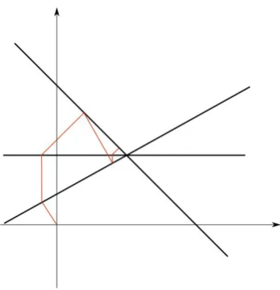
The demonstration of the idea can be shown in Figure 1.1.

(19)

[image:19.595.218.416.106.311.2]

1.3. THESIS STRUCTURE 5

Figure 1.1: Illustration of iteration steps when applying KM

Kaczmarz method has been used in signal and image processing, such as com-puted tomography [14]. Although Kaczmarz proved the method is convergent [20], the convergence rate of this method is difficult to obtain and hard to com-pare with other methods.

1.3 Thesis Structure

In the previous sections, we introduced the traditional Kaczmarz method. In this thesis, we are going to develop the traditional Kaczmarz method into randomised Kaczmarz method (RKM), accelerated RKM, RKM for solving systems of lin-ear inequalities, randomised sparse Kaczmarz method (RSKM), and exact-step randomised sparse Kaczmarz method (ERSKM).

We will start by explaining the RKM algorithm for exact data and its con-vergence properties, and application of it towards the noisy data in Chapter 2. In addition, our methodology involving the accelerated randomised Kaczmarz method will also be explicitly explained in that chapter. We will present an extension of RKM into solving systems of linear inequalities.

(20)

method and also analyse convergence properties of both exact and noisy data cases.

In Chapter 4, applying the methodologies described and explained in Chap-ter 2 and ChapChap-ter 3, we will present and discuss the results of our numerical experiments.

(21)

Chapter 2 Randomised Kaczmarz Method

2.1 Motivating Example

Recall in Chapter 1, we derived the Kaczmarz Method. Firstly let us have a look on an example on solving linear equations.

Example 2.1. Consider the linear systems given by



 

1 −2

0 1

1 1



 

x1

x2

!

=



 

−2 2 4



 .

For this problem, we conduct the KM with initial guess (x1, x2)T = (0,0)T so we

have those steps shown by red lines in following Figure 2.1.

However, if we change the order of the rows of the matrix to reformulate the problem as



 

0 1

1 −2

1 1



 

x1

x2

!

=



 

2 −2

4



 .

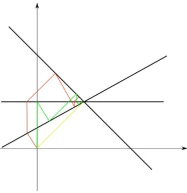
This is equivalent to the original problem. By performing KM on this system with the same initial guess, the iteration steps go through as shown by the green lines in Figure 2.1.

We can directly see from the Figure 2.1 that the second system has a faster convergence rate, though they are equivalent. If the first step in KM is performed by projecting the initial guess (0,0)T _{onto the hyperplane}_h(1_,₁₎T_,₍_x

1, x2)Ti= 4,

we can even directly get the solution. This shows that the order of rows of matrix have a significant influence to the speed of convergence.

(22)

[image:22.595.187.374.118.311.2]

Figure 2.1: Iteration steps when applying KM in different order of matrix rows

The Kaczmarz Method iterates through the rows of A by a certain order leading to the dramatically high dependence of its convergence rate on the order. Intuitively, we can have the row chosen randomly in each iteration to avoid the impact of the order. The index chosen in the iteration can be viewed as a random variable.

2.2 Definitions and Construction

How shall we allocate probabilities to each hyperplane formulated by rows of a matrix? We can simply assign a probability to each row uniformly, that is, with equal probability 1/m. Also, another method is that we can assign a probability to each row related to the “distance” between the row vector and zero, that is, the probability is proportional to the 2-norm square of each row. Hence, for better allocation of probabilities, we introduce the concept of Fr¨obenius norm (F-norm) of a matrix, the square root of the sum of all entries’ square of the matrix, which is equal to the sum of each row’s 2-norm square.

Definition 2.2. The Frobenius norm (F-norm) of a matrixA∈_Rm×n _{is denoted}

by ||A||F, and is defined by

||A||F :=

v u u t

n

X

i=1

m

X

j=1

(23)

2.2. DEFINITIONS AND CONSTRUCTION 9

where aij indicates the element of the matrixA in its ith row and jth column.

By using F-norm ||A||F, we can thus define P(ik =i) =

||ai||22

||A||2

F. We can check

that sum of each row’s probability Pm

i=1P(ik = i) = 1. From here, we can

construct the randomised Kaczmarz Method based on Algorithm 1 as follows.

Algorithm 2 (RKM). Given an initial guess x0, we have the iteration method

xk+1=xk+

br(k)− har(k), xki

||ar(k)||22

ar(k),

where the indexr(k)is drawn independent and identically distributed (i.i.d.) from the index set {1,2, ..., m} with the probability for theith row given by

P(r(k) = i) = ||ai||

2 2

||A||2

F

.

Instead of a certain preassigned order in the Kaczmarz’s method, the ran-domised Kaczmarz method sweeps the rows selected randomly with the proba-bility proportional to the 2-norm square of the row vectors of the matrix.

Here, some definitions are given for better discussion for the convergence rate in the following section.

Definition 2.3. The spectral norm of matrix A is ||A||2, the largest singular

value ofA, i.e.

||A||2 = (the maximum eigenvalue of (AHA)1/2,

where AH _{is the conjugate transpose of} _A_{. We will also use} _A† _{to denote the}

Moore-Penrose pseudoinverse of A, see [35].

Let σ1 ≥ σ2 ≥ · · · ≥ σr > 0 be all the nonzero singular values of A. It is

known that

kAk2 =σ1, kA†k2 =

1 σr

and kAkF =

q

σ2

1 +· · ·+σ2r. (2.1)

When solving a linear system, we need to measure how sensitive the answer is to perturbations in the input data and to roundoff errors made during the solution process. For this purpose, we need the concept of a condition number [32].

(24)

Definition 2.5. The scaled condition number is κ(A) := ||A||F||A†||2.

Using (2.1) we can easily derive that √

n≤κ(A)≤√nk(A).

2.3 Convergence Properties of RKM

Because the indexr(k) is a random variable in the randomised Kaczmarz Method, we will analyse its convergence and derive its convergence rate in terms of the expectation _E[||xk+1 −x∗||2], where x∗ denotes a solution of Ax = b and E[·]

denotes expectation with respect to the random row index selection.

2.3.1 Exact Data

In this section, we derive the convergence rate for the randomised Kaczmarz method when the data is given exactly. The following lemma is the key step.

Lemma 2.6. Let A have full column rank and assume the linear system Ax=b is consistent. Let x∗ be the solution of Ax=b. For any x let

x†=x+bi− hai, xi kaik22

ai

with i drawn from the index set {1,2,· · · , m} with the probability for the ith row given by kaik22/kAk2F. Then

E[kx+−x∗k2]≤ 1−κ(A)−2kx−x∗k2.

Proof. Since Ais of full column rank, there holds A†A=I. Thus, for anyz ∈_C, we have

kzk2 2 =||A

†

Az||2 2 ≤ kA

†_k2 2kAzk

2 2

=kA†k2₂

m

X

i=1

|hai, zi|2

Thus

m

X

i=1

|hz, aii|2 ≥

kzk2 2

kA†_k2 2

(25)

2.3. CONVERGENCE PROPERTIES OF RKM 11

By invoking the definition of the scaled condition number κ(A), we have

m

X

i=1

|hz, aii|2 ≥

||z||2 2||A||2F

κ(A)2 .

Rearranging the terms gives

m

X

i=1

kaik22

kAk2

F

hz, ai ||ai||

i 2

≥ kzk2 2κ(A)

−2 _(2.2)

Let Z be the random vector defined by

Z = ai kaik2

with probability kaik

2 2

kAk2

F

.

Then it follows from (2.2) that

E[|hz, Zi|2]≥ ||z||22κ(A)

−2_. _(2.3)

By the definition of x+ we can see thatx+ is the projection ofx onto the hyper-planehai, xi=bi. Thusx+−xis orthogonal to this hyperplane. Becausex∗ is on

this hyperplane, x+−xis orthogonal to x+−x∗. Therefore, by the Pythagorean theorem, we have

||x+−x∗||2 2+||x

+₋_x_||2

2 =||x−x

∗_||2 2.

This implies that

E[kx+−x∗k2] =kx−x∗k2−E[kx+−xk2]. (2.4) Note that

x+−x= bi− hai, xi kaik22

ai =

hai, x∗i − hai, xi

kaik22

ai

=

ai

kaik2

, x∗−x

ai

kaik2

.

We have

kx+−xk=

ai

kaik2

, x∗−x

.

Therefore, it follows from the definition of Z and (2.3) that

(26)

Using Lemma 2.6, we can easily derive the following convergence rate result for RKM with exact data.

Theorem 2.7. LetA have full column rank and assume the linear systemAx=b is consistent. Letx∗ be the solution ofAx=b. Then the sequence {xk}generated

by Algorithm 2 converges to x∗ in expectation, with the average error E[kxk−xk22]≤(1−κ(A)

−2₎k_||_x

0−x∗||22.

Proof. According to the definition of xk, we may apply Lemma 2.6 to conclude

that

E[kxk−x∗k22|xk−1]≤(1−κ(A)−2)kxk−1−x∗k22.

Now we take the full expectation on the both sides of the above equation to obtain

E[kxk−x∗k22]≤(1−κ(A)

−2

)_E[kxk−1−x∗k22].

By recursively using this inequality, we have E[kxk−x∗k22]≤(1−κ(A)

−2₎

E[||xk−1−x∗||22]

≤(1−κ(A)−2)2_E[||xk−2−x∗||22]

≤ · · ·

≤(1−κ(A)−2)kkx0−x∗k22.

2.3.2 Noisy Data

In practical applications, the data b is usually obtained by measurement, and it could be corrupted by noise. Thus, instead of b, we have a noisy data b+η with an error vector η added to b. Consequently, instead of the consistent linear system Ax=b, we may need to consider the linear system

Ax ≈b+η.

For this noisy system, there may be no solution, so we do not expect it to be consistent. However, the randomised Kaczmarz method is still applicable to generated an iterative sequence which is formulated as follows.

Algorithm 3 (RKM with noisy data). Given an initial guess x˜0 =x0, we have

the iteration method ˜

xk+1 = ˜xk+

br(k)+ηr(k)− har(k),x˜ki

||ar(k)||22

(27)

where the indexr(k)is drawn independent and identically distributed (i.i.d.) from the index set {1,2, ..., m} with the probability for theith row given by

P(r(k) = i) = ||ai||

2 2

||A||2

F

.

We have the following error estimate for the randomised Kaczmarz method with noisy data.

Theorem 2.8. LetAbe of full column rank and assume that the systemAx=bis consistent. Let x∗ be the solution of Ax=b. Let {˜xk} be generated by Algorithm

3 using a noisy data b+η. Then there holds

E[k˜xk−x∗k22]≤(1−κ(A))

k_k|

x0−x∗k22 +

kηk2 2

σmin(A)2

,

where the expectation is taken over the choice of rows in the algorithm, and σmin(A) denotes the smallest nonzero singular value of A.

Proof. Let xk denote the projection of ˜xk−1 onto the hyperplane Hi = {x :

hai, xi=bi}. It then follows from Lemma 2.6 that

E[kxk−x∗k22]≤(1−κ(A)

−2_)k˜

xk−1 −x∗k22. (2.5)

According to the definition of ˜xk, we can see that ˜xk is the projection of ˜xk−1 to

the hyperplane ˜Hi = {a :hai, xi= bi +ri}. Then xk −x˜k−1 is perpendicular to

Hi and ˜xk−x˜k−1 is perpendicular to ˜Hi. Both Hi and ˜Hi are parallel with the

same normal vector ai. Thus both xk−x˜k−1 and ˜xk−x˜k−1 are parallel to ai.

Consequently ˜xk−xk is parallel toai. We can write ˜xk−xk =tai for some scalar

t. Then

tkaik22 =hai, taii=hai,x˜k−xki=hai,x˜ki − hai, xki=bi+ηi−bi =ηi.

This shows that t=ηi/kaik22 and hence

˜

xk−xk =

ηi

kaik22

ai.

Note that xk −x∗ is in Hi which has the normal vector ai. Thus xk−x∗ and

˜ xk₋_x

k are perpendicular to each other. By the Pythagorean theorem, it follows

that

kx˜k−x∗k22 =kxk−x∗k22+k˜xk−xkk22.

Taking the conditional expectation on knowing ˜xk−1 gives

(28)

Note that k˜xk−xkk2 =|ηi|/kaik2, we have

E[k˜xk−xkk22|˜xk−1] =

m

X

i=1

P(r(k) = i) |ηi|

2

kaik22

=

m

X

i=1

kaik22

kAk2

F

|ηi|2

kaik22

= kηk

2 2

kAk2

F

.

Therefore

E[kx˜k−x∗k22|˜xk−1] =E[kxk−x∗k22|˜xk−1] +

kηk2 2

kAk2

F

.

In view of (2.5) we then have

E[k˜xk−x∗k22|˜xk−1]≤(1−κ(A)−2)k˜xk−1−x∗k22+

kηk2 2

kAk2

F

.

By taking the full expectation on the both sides it yields

E[k˜xk−x∗k22]≤(1−κ(A)

−2

)_E[k˜xk−1−x∗k22] +

kηk2 2

kAk2

F

.

Now we can apply this inequality recursively to obtain

E[k˜xk−x∗k22]≤(1−κ(A)

−2₎k_k_x

0−x∗k22

+ 1 + (1−κ(A)−2) +· · ·+ (1−κ(A)−2)k−1 kηk

2 2

kAk2

F

≤(1−κ(A)−2)kkx0−x∗k22+

1

1−(1−κ(A)−2₎

kηk2 2

kAk2

F

= (1−κ(A)−2)kkx0−x∗k22+κ(A) 2 kηk

2 2

kAk2

F

= (1−κ(A)−2)kkx0−x∗k22+kA

†_k2 2kηk

2 2.

Note that kA†k2 = 1/σmin(A), we therefore complete the proof.

2.3.3 Pre-asymptotic Convergence Properties

Theorem 2.7 gives error estimates in expectation for any iterate xk and the

con-vergence rate is determined by κ(A). For ill-conditioned problems, the condition number κ(A) can be very huge, and thus Theorem 2.7 predicts a very slow con-vergence. However, in practice, RKM converges rapidly during the initial stage of iterations. The estimate in Theorem 2.8 is also deceptive for noisy data due to the presence of the term kηk2

2/σmin(A)2, which implies blowup at the very

(29)

In this section, we will provide an explanation on the fast empirical con-vergence behaviour of the randomised Kaczmarz method by analysing its pre-asymptotic convergence behaviour and showing that the low-frequency error (with respect to the right singular vectors) decays faster during the first iterations than the high-frequency error.

To start, let the singular value decomposition (SVD) of A∈_Rm×n _{given by}

A=UΣVT, U ∈_Rm×m, V ∈_Rn×n. U =    uT 1 .. . uT_n

   V T =    vT 1 .. . v_mT



 

where U and V are orthogonal matrices whose columns are called the left and right singular vectors of A, and Σ∈_Rm×b _{is diagonal with the nonzero elements}

being the singular values of A, ordered non-increasingly by σ1 ≥ · · · ≥ σr > 0

with r≤min{m, n} [38].

Given a frequency cut-off number L with 1 ≤ L ≤ n, we can define two subspaces of _Rn _by

L = span{v1,· · · , vL}, H= span{vL+1,· · · , vm}

denoting by low frequency and high frequency solution spaces. L and H are orthogonal.

For any vector z ∈_Rm_{, there exists a unique decomposition}

z =PLz+PHz,

where PL and PH are the orthogonal projection operators onto L and H

respec-tively, defined by:

PLz = L

X

i=1

hvi, zivi, PHz = m

X

i=L+1

hvi, zivi.

We have the following lemmas based on SVD properties.

Lemma 2.9. For any eL∈ L and eH ∈ H, there hold

σL||eL|| ≤ ||AeL|| ≤σ1||eL||, ||AeH|| ≤σL+1||eH||, hAeL, AeHi= 0.

Proof. Since eL∈ L, we have

eL = L

X

i=1

heL, viivi, AeL= L

X

i=1

(30)

Therefore

keLk22 =

L

X

i=1

|hel, vii|2, kAeLk22 =

L

X

i=1

σ2_i|heL, vii|2

from which we immediately have σLkeLk2 ≤ kAelk2 ≤ σ1keLk2. By similar

argument we can show that kAeHk2 ≤σL+1keHk2 for eH ∈ H. Note that L and

H are invariant under AA_{, i.e.}

A∗A(L)⊂ L, A∗A(H)⊂ H. Thus

hAeL, AeHi=hA∗AeL, eHi= 0

because A∗AeL∈ L,eH ∈ H, and L and H are orthogonal.

Lemma 2.10. For i= 1,· · · , n, there hold

||PHai||2 ≤σL2+1,

n

X

i=1

||PHai||2 ≤ r

X

j=L+1

σ2_j.

Proof. Since A=    a1 .. . an   =    uT 1 .. . uT_n



 ΣV

T

we have ai =uTiΣVT. Note also that

VTvj =



 

vT

1vj

.. . v_mTvj

  =          0 .. . 1 .. . 0         

=ej.

Therefore

PHai = m

X

j=L+1

hvj, aiivj = m

X

j=L+1

(aT_i vj)vj

=

m

X

j=L+1

(uT_i ΣVTvj)vj = m

X

j=L+1

(uT_i Σej)vj

=

m

X

j=L+1

(uT_i σjej)vj = m

X

j=L+1

(31)

Consequently

||PHai||22 =

m

X

j=L+1

σ_j2hui, eji2 ≤σ2L+1

m

X

j=L+1

hui, eji2 ≤σL2+1kuik2 =σ2L+1.

The second statement can be proved similarly.

Let the error of kth iteration be ek := xk−x∗, where xk is the kth iterate,

and x∗ is the exact solution. We then have the following theorem on the pre-asymptotic convergence for Algorithm 2 concerning the situation without noise.

Theorem 2.11. Let c1 = _||_AσL_||2 F

, and c2 = _k_A1_k2 F

Pr

i=L+1σ 2

i. Then there hold

E[||PLek+1||2|ek]≤(1−c1)||PLek||2+c2||PHek||2,

E[||PHek+1||2|ek]≤c2||PLek||2+ (1 +c2)||PHek||2.

Proof. Adjust the algorithm formula for the error ek and ek+1. Without losing

generality, let i:=r(k). Then

xk+1−x∗ =xk−x∗+

bi− hai, xki

||ai||22

ai.

Therefore

ek+1 =ek+

bi− hai, xki

||ai||22

ai =ek+

hai, x∗i − hai, xki

||ai||22

ai

=ek+

hai, x∗−xki

||ai||22

ai =ek−

hai, eki

||ai||22

ai

=

I− aia

T i

||ai||22

ek.

Errorek can be decomposed into the projections ontoLandH, i.e. ek=eL+eH,

where eL:=PLek and eH :=PHek. Then we have

PLek+1 =PLek−

hai, eki

||ai||22

PLai =eL−

hai, eki

||ai||22

PLai.

Based on property hPLai, eLi=hai, eLi, we can obtain

||PLek+1||22 =||eL−

hai, eki

||ai||22

PLai||22

=||eL||22−

2hai, eki

||ai||22

hPLai, eLi+||

hai, eki

||ai||22

PLai||22

=||eL||22−

2hai, eki

||ai||22

hai, eLi+

hai, eki2

||ai||42

(32)

≤ ||eL||22−

2hai, eki

||ai||22

hai, eLi+

hai, eki2

||ai||22

=||eL||22−

2hai, eki

||ai||22

hai, eLi+

hai, eL+eHi2

||ai||22

=||eL||22−

2hai, eL+eHi

||ai||22

hai, eLi

+hai, eLi

2₊_h_a

i, eHi2+ 2hai, eLihai, eHi

||ai||22

=||eL||22+

hai, eHi2 − hai, eLi2

||ai||22

.

By taking the expectation conditional on knowing ek and using Lemma 2.9, it

follows that

E[||PLek+1||22|ek] ≤ ||eL||22+

n

X

i=1

||ai||22

||A||2

F

−hai, eLi2 +hai, eHi2

||ai||22

= ||eL||22+

1 ||A||2

F

(−

n

X

i=1

hai, eLi2+ n

X

i=1

hai, eHi2)

= ||eL||22+

1 ||A||2

F

(−||AeL||22+||AeH||22)

≤ (1−c1)||PLek||2+c2||PHek||2

Similarly we have

PHek+1 =eH −

PHai

||ai||22

PHai.

Then

||PHek+1||22 =||eH −

hai, eki

||ai||22

PHai||22

=||eH||22−

2hai, eki

||ai||22

hPHai, eHi+||

hai, eki

||ai||22

PHai||22

≤ ||eH||22−

2hai, eki

||ai||22

hai, eHi+

||PHai||22

||ai||42

||ai||22||ek||22

=||eH||22−

2hai, eki

||ai||22

hai, eHi+

||PHai||22

||ai||22

(||eL||22+||eH||22)

By taking the conditional expectation on both sides and using Lemma 2.9 and Lemma 2.10, we can obtain

E[||PHek+1||22|ek]

≤ ||eH||22−

n

X

i=1

||ai||22

||A||2

F

_2h

ai, eki

||ai||22

hai, eHi+

||PHai||22

||ai||22

(||eL||22+||eH||22)

(33)

2.4. ACCELERATED RANDOMISED KACZMARZ METHOD 19

=||eH||22−

2||AeH||22

||A||2

F

+

n

X

i=1

||PHai||22

||A||2

F

(||eL||22+||eH||22)

≤c2||eL||22+ (1 +c2)||eH||22.

By Theorem 2.11, the decay of the error_E[[kPLek+1k2|ek] is largely determined

by the factor 1−c1 and only mildly affected bykPHekk2 by a factor c2. By taking

expectation of both sides of the estimates in Theorem 2.11, we can obtain E[kPLek+1k2]≤(1−c1)E[kPLekk2] +c2E[kPHekk2],

E[kPHek+1k2]≤c2E[kPLekk2] + (1 +c2)E[kPHekk2]

By using this estimate recursively, it follows that E[kPLekk2]

E[kPHekk2]

!

≤Dk kPLe0k

2

kPHe0k2

!

, D= 1−c1 c2 c2 1 +c2

!

.

By studying the spectral property of the matrix D, one can obtain for α := c2/c1 1 the following approximate error propagation for k =O(1):

E[kPLekk2]≈(1−c1)kkPLe0k2+α(1−(1−c1)k)kPHe0k2,

E[kPHekk2]≈α(1−(1−c1)k)kPLe0k2+ (1 +kαc1)kPHe0k2

which explains the fast decay property of the randomised Kaczmarz method dur-ing the first iterations, see [18] for details.

2.4 Accelerated Randomised Kaczmarz method

By applying the Nesterov’s acceleration strategy [29] to the RKM, in this section we consider an accelerated version of RKM for solving the consistent linear system

Ax=b

with the assumptions on A as before. Moreover, we assume that the rows of A are normalised in the sense that kajk2 = 1 for j = 1,· · · , m.

2.4.1 Construction

For the minimisation problem

min

x∈Rn

(34)

with a differentiable objective function f(x), the gradient method takes the form

xk+1 =xk−θk∇f(xk), k = 0,1,· · · ,

where θk is the step size. Nesterov proposed several schemes to accelerate the

gradient method [29], one of the acceleration scheme can be formulated as follows yk =αkvk+ (1−αk)xk,

xk+1 =yk−θk∇f(yk),

vk+1 =βkvk+ (1−βk)yk−γk∇f(yk)

(2.6)

with suitable choices of αk,βk, γkand θk. We can use this strategy to propose an

accelerated randomised Kaczmarz method (ARKM) by modifying the projection step of RKM in Algorithm 2, that is, instead of defining xk+1 by

xk+1 =xk+

bi− hai, xki

kaik22

ai

directly, we will use an analog of the three step strategy in (2.6) to define xk+1.

This leads to the following accelerated randomised Kaczmarz method.

Algorithm 4 (ARKM). Given an initial guess x0, let v0 = x0, γ−1 = 0, and

λ ∈[0, λmin], where λmin is the smallest non-zero singular value of A, that is, the

minimum eigenvalue of AT_A_{. For}_k _{= 0}_,₁_,_{· · ·} _{we choose} _γ

k to be the larger root

of

γ_k2− γk m =

1− γkλ m

γ_k2₋₁ and define

αk=

m−γkλ

γk(m2−λ)

βk= 1−

γkλ

m ;

yk=αkvk+ (1−αk)xk;

xk+1 =yk+

bi−aTi yk

kaik2

ai;

vk+1 =βkvk+ (1−βk)yk+γk

bi−aTi yk

kaik22

ai,

(35)

From this we can develop a more efficient algorithm by calculating the pa-rameters. Let

gk :=

aT_i yk−bi

||ai||22

ai.

Then we can represent parameters of Algorithm 4 in a new way for developing a equivalent algorithm with less cost. Recall the last two iterate steps of Algorithm 4, we have

vk+1 =βkvk+ (1−βk)yk−γkgk, xk+1 =yk−gk.

Recall also that yk = αkvk + (1 −αk)xk, we have vk = _α1

k(yk −(1− αk)xk).

Therefore

vk+1 =

βk

αk

yk−(1−αk)xk) + (1−βk)yk−γkgk

=

βk

αk

+ 1−βk

yk−

βk(1−αk)

αk

xk−γkgk.

Similarly, substitute thisvk+1 and xk+1 =yk−gk into the formula

yk+1 =αk+1vk+1+ (1−αk+1)xk+1

for yk+1, we can obtain

yk+1 =αk+1

βk

αk

+ 1−βk

yk−

βk(1−αk)

αk

xk−γkgk

+ (1−αk+1)(yk−gk)

=

1 + 1−αk αk

αk+1βk

yk−

1−αk

αk

αk+1βkxk

−(1−αk+1+αk+1γk)gk.

According to the formulae of αk and βk in Algorithm 4, we have

1−αk

αk

βk =

1 αk −1 βk =

γk(m2−λ)

m−γkλ

−1 1− γkλ m

=

γk(m2−λ)

m−γkλ

−1

m−γkλ

m

= γk(m

2₋_λ₎

m −

m−γkλ

m

= γkm

2₋_m

(36)

Thus

yk+1 =αk+1(1−mγk)xk+ (1−αk+1+mαk+1γk)yk−(1−αk+1+αk+1γk)gk.

(2.7) According to (2.7) we can see that there is no need to calculate βk and vk. This

leads to the following equivalent but more efficient algorithm.

Algorithm 5 (EARKM). Given an initial guess x0, let v0 = x0, γ−1 = 0, and

λ ∈ [0, λmin], where λmin is the smallest non-zero singular value of A, that is,

the minimum eigenvalue of ATA. For k = 0,1,· · ·, generate γk and αk as in

Algorithm 4, and define sk =

aT

i yk−bi

||ai||22

; gk =skai;

yk+1 =αk+1(1−mγk)xk+ (1−αk+1+mαk+1γk)yk

−(1−αk+1+αk+1γk)gk;

xk+1 =yk−gk,

where i is drawn from {1,2,· · · , m} with uniform probability distribution.

2.4.2 Convergence Properties

Now we will give the convergence analysis on the accelerated randomised Kacz-marz method. For a positive semi-definite metric B, we set

||x||B :=

p

trace(XT_BX₎_.

Theorem 2.12. Consider Algorithm 4. Let σ1 = 1 +

√ λ

2m and σ2 = 1− √

λ 2m. Then we have

E[kvk−x∗k2(AT_A₎+]≤

4kx0−x∗k2₍_AT_A₎+

(σk

1 +σ2k)2

, _E[kxk−x∗k2]≤

4m2_k_x

0−x∗k2₍_AT_A₎+

(σk

1 +σ2k)2

for k = 1,2,· · ·.

The proof of Theorem 2.12 is based on a series lemmas.

Lemma 2.13. For a row normalised matrix A ∈_Rm×n _{there holds} _λ

(37)

Proof. By the definition ofλmin, there is anx6= 0 such thatATAx=λminx. Note

that

A=



 

aT₁ .. . aT m  

 =⇒ A

T_A₌_a

1aT1 +· · ·+amaTm.

We have

λminx= (a1aT1 +· · ·+amaTm)x.

Therefore

λminkxk2 =h(a1aT1 +· · ·+amaTm)x, xi= (a T

1x)

2₊_{· · ·}_{+ (}_aT mx)

2

≤ ka1k22kxk 2

2+· · ·+kamk22kxk 2 2

=mkxk2 2.

Since kxk2 6= 0, we must have λmin ≤m.

Lemma 2.14. For the sequence{γk}, {αk} and {βk} defined in Algorithm 4, we

have

γk−1 ≤γk≤

1 √

λ, γk≥ 1

m and 0≤αk, βk ≤1 for all k ≥0.

Proof. We first show the assertion of {γk} by an induction argument. Since

γ−1 = 0, γ0 is the larger root of the equationγ2−γ/m = 0 and henceγ0 = 1/m.

By Lemma 2.13 we have λ ≤λmin ≤ m. Thus the assertion for γ0 follows. Now

we assume the assertion for γk for some k ≥ 0, and show that the assertion is

also true for γk+1. Consider the function

t(γ) :=γ2− 1−λγ

2

k

m γ−γ

2

k.

Clearly t(γ)→+∞as |γ| → ∞. Note that

t(1 m) =

1 m2 −

1−λγ_k2 m

1 m −γ

2

k =

λ m −1

γ_k2 ≤0

since λ/m2₋₁ _≤ _m/m2₋_{1 = 1}_/m₋₁_≤ _{0. This shows that} _t₍_γ_{) must have a}

root on [1/m,∞). Thus γk+1 ≥1/m by the definition of γk+1. Note also that

t(γk) =γk2−

1−λγ_k2

m γk−γ

2

k =−

γk(1−λγk2)

(38)

by the induction hypothesis on γk. We also have γk+1 ≥ γk by the definition of

γk+1. Moreover,

f(√1 λ) =

1 λ −

1

m√λ(1−λγ

2

k)−γ

2

k =

1 λ −

1 m√λ +γ

2

k

√ λ m −1

!

≥ 1 λ −

1 m√λ +

1 λ

√ λ m −1

!

= 0

since γ_k2 ≤1/√λ and√λ/m−1≤0. Note that t(γ) is a strong convex quadratic function, we must have t(γ)>0 for all γ >1/√λ. Therefore γk+1 ≤1/

√ λ. Using the assertion for {γk} and the definition of αk and βk, we can see

immediately that 0≤αk, βk≤1 for all k ≥0.

Lemma 2.15. Let U ∈_Rm×r _with _UT_U ₌_I_{. Let} _UT _{= [}_u

1, u2,· · · , um]. Then

kuik2 ≤1 for i= 1,· · · , m.

Proof. Let U = [˜u1,u˜2,· · · ,u˜r]. Then UTU = I implies that ˜uTiu˜j = 1 if i = j

and = 0 ifi6=j. LetW be the space spanned by{˜u1,· · · ,u˜r}. Then{˜u1,· · · ,u˜r}

is an orthonormal basis of W. Thus for any y∈_Rm_{, the projection of}_x _onto _W

is

PW(y) = r

X

i=1

(˜uT_i y)˜ui = r

X

i=1

˜

uiu˜Ti y=U U T

y.

Thus kUTyk2

2 =hU U

T_{y, y}_i₌_h_P

W(y), yi=hPW(y), PW(y)i=kPW(y)k22 ≤ kyk 2 2.

By taking y=ej which is the vector whose entries are zeros except thejth spot

where the entry is 1, we then obtain kujk22 =kU

T_e

jk22 ≤ kejk22 = 1.

Lemma 2.16. For every w∈_Rn_,

E[||ai(aTi w−bi)||2(AT_A₎+]≤

1

m||Aw−b||

2_,

(39)

Proof. By using the singular value decomposition, we can write A=UΣVT,

whereU ∈_Rm×r _satisfies_UT_U ₌_I_, _V _∈

Rn×r satisfiesVTV =I and Σ∈Rr×r is a positive diagonal matrix with r being the rank of A. Thus AT _{= (}_U_Σ_VT₎T ₌

VΣUT _{and hence}

ATA=VΣUTUΣVT =VΣ2VT.

Therefore the Moore-Penrose pseudoinverse of (AT_A_{) is (}_AT_A₎+ ₌ _V_Σ−2_VT_.

By taking the expectation with respect to i, and using the commutativity and linearity of trace, i.e.

trace(BC) = trace(CB), trace(B +C) = trace(B) +trace(C)

we have

E[||ai(aTi w−bi)||2(AT_A₎+]

= 1 m

m

X

i=1

trace (ai(aTi w−bi))T(ATA)+(ai(aTi w−bi))

= 1 m

m

X

i=1

trace (ATA)+(ai(aTi w−bi))(ai(aTiw−bi))T

= 1

m trace (A

T_A₎+

m

X

i=1

ai(aTi w−bi)2aTi

!

= 1

m trace (A

T_A₎+_AT _diag(_Aw₋_b₎_A

= 1

m trace(VΣ

−2_VT_V_Σ_UT _diag(_Aw₋_b₎2_U_Σ_VT₎

= 1

m trace(VΣ

−1_UT _diag(_Aw₋_b₎2_U_Σ_VT₎

= 1

m trace(ΣV

T_V_Σ−1_UT _diag(_Aw₋_b₎2_U₎

= 1

m trace(U

T _diag(_Aw₋_b₎2_U₎

= 1 m

m

X

i=1

(aT_i w−b)2||ui||2

≤ 1

m||Aw−b||

2_,

(40)

Lemma 2.17. Let x∗ be any solution of Ax = b, where A is assumed to be normalised. For any w∈ _Rn _let _p

i(w) be defined as the orthogonal projection of

w onto aT

i w=bi, i.e.

pi(w) :=w−

ai

||ai||2

(aT_i w−bi) = w−(aTi w−bi),

Then

E[||pi(w)−x∗||2] =||w−x∗||2−

1

m||Aw−b||

2_,

where the expectation is taken with respect to iwhich is uniformly distributed from the index set {1,· · · , m}.

Proof. Because Ax∗ =b and kaik= 1 for i= 1,· · · , m, we have

E[||pi(w)−x∗||2] =E[||w−ai(aTi w−bi)−x∗||2]

=||w−x∗||2₊

E[(aTi w−bi)2]−2E[hw−x∗, ai(aTi w−bi)i]

=||w−x∗||2₊

E[(aTi w−bi)2]−2E[haTi (w−x

∗₎_{, a}T

i w−bii

=||w−x∗||2₊

E[(aTi w−bi)2]−2E[(aTiw−bi)2]

=||w−x∗||2₋

E[(aTi w−bi)2]

=||w−x∗||2− 1 m

m

X

i=1

(aT_i w−bi)2

=||w−x∗||2₋ 1

m||Aw−b||

2_.

Lemma 2.18. Consider Algorithm 4. Let

rk =kvk−x∗k(AT_A₎+ and s_k =kx_k−x∗k.

Then there holds

E[rk2+1|k] +γ 2

kE[s

2

k+1|k]≤βkrk2+βkγk2−1s 2

k, (2.8)

where the expectation is conditioned on knowing all the previous k iterations. Proof. Recall that

vk+1=βkvk+ (1−βk)yk−γk(aTi yk−bi)ai,

here we used the normalisation kaik2 = 1. Then we have

r_k2₊₁ =||vk+1−x∗||(2AT_A₎+ =||βkvk+ (1−βk)yk−γk(aTiyk−bi)ai−x∗||2(AT_A₎+

(41)

where

I1 =||βkvk+ (1−βk)yk−x∗||2(AT_A₎+,

I2 =||γkai(aTi yk−bi)||2(AT_A₎+,

I3 =−2hβkvk+ (1−βk)yk−x∗,(ATA)+γkai(aTi yk−bi)i.

Now we consider these three terms separately. From Lemma 2.14 we know that 0 ≤ βk ≤ 1. Since the semi-norm || · ||2₍_AT_A₎+ is convex, by using convexity we

have

I1 =||βk(vk−x∗) + (1−βk)(yk−x∗)||2(AT_A₎+

≤βk||vk−x∗||2(AT_A₎+ + (1−βk)||yk−x∗||2(AT_A₎+.

Recall from the definition of βk that 1−βk=γkλ/m. Thus

I1 ≤βkr2k+

γkλ

m ||yk−x

∗_||2 (AT_A₎+.

Since in Algorithm 4 we take x0 = 0, we can show bu induction that xk, yk, vk

and x∗ are all in R(AT). Thus, by the definition of λmin we have

kyk−x∗k2(AT_A₎+ ≤

1 λmin

ky−xk2 2.

This together with λ ≤λmin gives

I1 ≤βkrk2+

γk

mkyk−x

∗_k2

2. (2.10)

Recall thatxk+1 is the projection of yk onto the plane{x:aTi x=b}, we may use

Lemma 2.16 and Lemma 2.17 to conclude that E[I2|k] =E[γk2||ai(aiTyk−bi)||2(AT_A₎+|k]≤

γ2

k

m||Ayk−b||

2 2

=γ_k2 ||yk−x∗||2−E[||xk+1−x∗||2|k]

=γ_k2 kyk−x∗k2−E[s2k+1|k]

. (2.11)

For I3 we have

E[I3|k] =−2γkhβkvk+ (1−βk)yk−x∗,(ATA)+E[ai(aTiyk−bi)]i

=−2γk

m hβkvk+ (1−βk)yk−x

∗

,(ATA)+

m

X

i=1

ai(aTi yk−bi)i

=−2γk

∗

,(ATA)+AT(Ayk−b)i

=−2γk

∗

,(ATA)+ATA(yk−x∗)i

=−2γk

∗

(42)

Recall that yk=αkvk+ (1−αk)xk, we have

vk =

1 αk

yk−

1−αk

αk

xk.

Thus

E[I3|k] =−

2γk

m βk 1 αk

yk−

1−αk

αk

xk

+ (1−βk)yk−x∗, yk−x∗

= 2γk m

x∗−yk+

1−αk

αk

βk(xk−yk), yk−x∗

=−2γk

m kyk−x

∗_k2₊2γk

m

1−αk

αk

βkhxk−yk, yk−x∗i.

Recall that

αk=

m−γkλ

γk(m2−λ)

and γ_k2− γk m =

1− γkλ m

γ_k2₋₁. We have

1−αk

αk

= m

2_γ

k−m

m−γkλ

= mγ

2

k−1

γk

.

Therefore

E[I3|k] =−

2γk

m kyk−x

∗_k2

+ 2βkγk2−1hxk−yk, yk−x∗i

=−2γk

m ||yk−x

∗_||2₊_β

kγk2−1 kxk−x∗k2− kyk−x∗k2− kxk−ykk2

=−

2γk

m +βkγ

2

k−1

kyk−x∗||2+βkγk2−1 kxk−x∗||2− kxk−ykk2

≤ −

2γk

m +βkγ

2

k−1

kyk−x∗||2+βkγk2−1kxk−x∗k2. (2.12)

Combining (2.10), (2.11) and (2.12) with (2.9) we obtain

E[rk2+1|k]≤βkrk2−γ

2

kE[s

2

k+1|k] +βkγk2−1s 2

k+

γ_k2− γk

m −βkγ

2

k−1

kyk−x∗k2.

According to the definition of γk andβk we haveγk2− γk

m −βkγ

2

k−1 = 0. Therefore

E[rk2+1|k]≤βkrk2−γ

2

kE[s

2

k+1|k] +βkγk2−1s 2

k.

and the proof is complete.

Lemma 2.19. Let {ak} and {bk} be two sequence of non-negative numbers with

a0 = 0, b0 6= 0 and

a2_k₊₁ =γ_k2b2_k₊₁, b2_k₊₁ = b

2

k

βk

(43)

where {βk} and {γk} are defined by Algorithm 4. Then ak ≥ak−1, bk≥bk−1 and

ak≥

b0

2(σ

k i −σ

k

2), bk≥

b0

2(σ

k

1 +σ

k

2)

for all k ≥1, where

σ1 = 1 +

√ λ

2m, σ2 = 1− √

λ 2m. Proof. Since 0< βk ≤1 and γk2−γk/m =βkγk2−1, we have

b2_k₊₁ = b

2

k

βk

≥b2_k

and

a2_k₊₁ =γ_k2b2_k₊₁ = γ

2 kb 2 k βk = γ 2 ka 2 k

βkγk2

= γ 2 ka 2 k γ2

k−γk/m

≥a2_k.

Therefore ak+1 ≥ak and bk+1 ≥bk for k≥0.

Next we derive the growth rate on ak and bk. We have

b2_k =βkb2k+1=

1− λ mγk

b2_k₊₁ =

1− λak+1 mbk+1

b2_k₊₁ =b2_k₊₁− λ

mak+1bk+1.

Thus λ

mak+1bk+1 =b

2

k+1−b 2

k = (bk+1+bk)(bk+1−bk)≤2bk+1(bk+1−bk).

Consequently

bk+1 ≥bk+

λ

mak+1 ≥bk+ λ

mak. (2.13)

Similarly, we have that Aa2_k₊₁

b2

k+1

− ak+1 mbk+1

=γ_k2− γk

m =βkγ

2

k−1 =βk

a2 k b2 k = a 2 k b2 k+1 . Thus

a2_k₊₁− 1

mak+1bk+1 =a

2

k

which implies that 1

mak+1bk+1 =a

2

k+1−a 2

k = (ak+1+ak)(ak+1−ak)≤2ak+1)(ak+1−ak).

Therefore

ak+1 ≥ak+

1

2mbk+1 ≥ak+ 1

(44)

Combining (2.13) and (2.14) we have ak+1

bk+1

!

≥D ak bk

!

, (2.15)

where

D= 1

1 2m λ

2m 1

!

.

Since all entries of D are non-negative, we may use (2.15) recursively to obtain ak

bk

!

≥Dk a0 b0

!

, (2.16)

From the characteristic equation

0 = det(σI −D) = (σ−1)2− λ 4m2,

of D, we can see that Dhas two distinct eigenvalues σ1 = 1 +

√ λ

2m, σ2 = 1− √

λ 2m. Direct calculation shows that

1 √

λ

!

and 1

−√λ

!

are eigenvectors of D corresponding to σ1 and σ2 respectively. Therefore

D= √1 1

λ −√λ

!−1

σ1 0

0 σ2

!

1 1

√

λ −√λ

!

,

Consequently

Dk= √1 1 λ −√λ

!−1

σ1 0

0 σ2

!k

1 1

√

λ −√λ

!

= 1 2

1 √1

λ

1 −_√1

λ

!

σk

1 0

0 σk

2

!

1 1

√

λ −√λ

!

= 1 2

σk₁ +σk₂ σ₁k−σ₂k σk₁ −σk₂ σ₁k+σ₂k

!

,

Combining this with (2.16) yields ak ≥

a0

2 (σ

k

1 +σ

k

2) +

b0

2(σ

k

1 −σ

k

2),

bk ≥

a0

2 (σ

k

1 −σ

k

2) +

b0

2(σ

k

1 +σ

k

2).

(45)

2.5. RKM SOLVING INEQUALITIES 31

Now we are ready to complete the proof of Theorem 2.12.

Proof of Theorem 2.12. By taking the full expectation on the equation (2.8) in Lemma 2.18, we have

E[r2k+1] +γ 2

kE[s

2

k+1]≤βk E[r2k] +γ

2

k−1E[s 2

k]

. (2.17)

Recursively using this equation we can obtain

E[r2k] +γk2−1E[s2k]≤β0· · ·βk−1 E[r02] +γ−21E[s20]

=β0· · ·βk−1r02.

Let {ak} and {bk} be the sequences defined in Lemma 2.19. Then we have

β0· · ·βk−1 =

b2 0

b2

k

.

Recall that γk ≥1/m fork ≥0, we therefore obtain

E[rk2] +

1 m2E[s

2

k] =

b2 0

b2

k

r2₀.

By making use of the estimate of{bk}given in Lemma 2.19 we thus complete the

proof.

2.5 RKM Solving Inequalities

In this section, we consider to generalise the randomised Kaczmarz method for linear equations to solve system of linear inequalities of the form

aT_ix≤bi, i∈ I,

aT_i x=b1, i∈ E,

(2.18)

whereI is the set of indices of inequalities andE is the set of indices of equalities, we assume thatI andE are disjoint and form a partition of the set{1,2,· · · , m}. We will modify Algorithm 2 so that it can be used to solve (2.18). We will letA to be the matrix whose rows areaT

i with i∈ I ∪ E. We will also use the notation

x+ := max{x,0}

(46)

Algorithm 6. Consider the systems of linear inequalities (2.18). Let x0 be an

arbitrary initial point. For k = 0,1,· · ·, compute βk =

(

(aixk−bi)+, i∈ I,

aT_i xk−bi, i∈ E,

xk+1 =xk−

βk

||ai||22

ai,

where, at each iterationk, the indexiis drawn independently from the set{1,2,· · · , m} with probability

P(i=j) = ||aj||

2 2

||A||2

F

.

In order to analyse Algorithm 6, we need the following theorem due to Hoffman [16] which tells about the distance between any x and a non-empty set of a polyhedron, which may be a solution set of a linear inequality system, is bounded by a linear function.

Theorem 2.20 (Hoffman). There is a constantL such that, for any x∈_Rn _and

b ∈_Rm _{such that the solution set}

Sb :={x∈Rn :aTi x≤bi for i∈ I and aTi x=bi for i∈ E}

of the system of linear inequalities (2.18) is nonempty, there holds d(x, Sb)≤L||e(Ax−b)||,

where d(x, Sb) denotes the distance from x to Sb, i.e.

d(x, Sb) = inf z∈Sb

kx−zk2,

and e:_Rm _→

Rm is a function defined by e(y)i =

(

max{yi,0}, i∈ I,

yi, i∈ E.

The smallest constant L is called the Hoffman constant.

From Theorem 2.20 we can obtain the convergence properties about Algorithm 6 by observing that βk =e(Axk−b)i.

Theorem 2.21. Assume that the system of linear inequalities (2.18) has a nonempty solution set S. Then Algorithm 6 converges linearly in expectation, that is,

E[d(xk, S)2]≤

1− 1

L2_||_A_||2

F

k

d(x0, S)2,

(47)

2.5. RKM SOLVING INEQUALITIES 33

Proof. Let PS denote the projection operator ontoS. Then

d(x, S) =kx−PS(x)), ∀x∈ |mathbbR n

.

By the definition og distance function and the factPS(xk)∈S we have

d(xk+1, S)2 ≤ kxk+1−PS(xk)k2.

Since xk+1 =xk− _k_aβk

ik2ai, we have

d(xk+1, S)≤

xk−PS(xk)−

βk

kaik2

ai 2

=kxk−PS(xk)k2+

β_k2 kaik2

−2 βk kaik2

aT_i (xk−PS(xk))

=d(sk, S)2 +

β_k2 kaik2

−2 βk kaik2

aT_i (xk−PS(xk)). (2.19)

Note that PS(xk)∈S. For i∈ I we have aiTPS(xk)≤bi. Since βk ≥0, we must

have

βk

kaik2

aT_i (xk−PS(xk))≥

βk

kaik2

(aT_i xk−bi) =

β_k2 kaik2

.

For i∈ E we have aT_i PS(xk) =bi and thus

βk

||ai||2

aT_i(xk−PS(xk)) =

βk

||ai||22

(aT_i xk−bi) =

β2

k

||ai||22

.

Combining the above two cases with (2.19), it follows that

d(xk+1, S)2 ≤d(xk, S)2−

β_k2 kaik2

=d(x, S)2 −[e(Axk−b)i]

2

kaik2

.

Therefore, by taking the conditional expectation on knowing x)k we have

E[d(xk+1, S)2|xk]≤d(xk, S)2−E

[e(Axk−b)i]2

||ai||2

=d(xk, S)2− m

X

i=1

kaik2

kAk2

F

[e(Axk−b)i]2

kaik2

=d(xk, S)2−

1 kAk2

F m

X

i=1

[e(Axk−b)i]2

=d(xk, S)−

1 kAk2

F

(48)

With the help of Theorem 2.20, it yields

E[d(xk+1, S)2|xk]≤d(xk, S)2−

1 L2_k_A_k2

F

d(xk, S)2

=

1− 1

L2_k_A_k2

F

d(xk, S)2.

Taking the full expectation gives

E[d(xk+1, S)2] =

1− 1

L2_k_A_k2

F

E[d(xk, S)2].

Recursively using this inequality we then obtain

E[d(xk, S)2]≤

1− 1

L2_k_A_k2

F

k

E[d(x0, S)2]

=

1− 1

L2_k_A_k2

F

k

d(x0, S)2

(49)

Chapter 3 Randomised Sparse Kaczmarz

Method

In this chapter, we focus on problems of recovering sparse solution of systems of linear equations. Sparsity indicates that most entries are zero. This characteristic runs prevalent in real-world situations. For instance, in computational biology, the alignment of DNA sequences from similar ancestors has its entries largely zeros [9]. Moreover, it is widely-appeared not only on statistical learning [36], but on signal processing, [17] especially image signal processing, as well.

Now, let us consider the linear system with sparse solutions

Ax=b, (3.1)

where A∈_Rm×n_{. The interest is to find a solution as sparse as possible. Here a}

vector is said to be sparse if most of its entries are zeros. Given a vectorx∈_Rn_,

its support is defined as

supp(x) :={i∈ {1,· · · , n}:xj 6= 0}.

The number of elements in supp(x) is called the sparsity level ofxand is denoted bykxk0. A natural procedure for finding a sparse solution of (3.1) is of course to

solve the constrained minimisation problem

min{kxk0 :Ax=b}. (3.2)

Unfortunately, due to the non-smoothness and non-convexity of kxk0, this

min-imisation problem becomes extremely difficult to solve. Instead of solving (3.2) directly, one may consider its convex relaxation

min{kxk1 :Ax=b}, (3.3)

(50)

where k · k1 denotes the `1-norm, i.e.

kxk1 =

n

X

i=1

|xi|.

It turns out that the model (3.3) can recover sparse solution very well, see [6], and many algorithms have been developed for solving (3.3. Because the function kxk1 is not strong convex, it poses numerical challenges for solving (3.3). In order

to develop fast numerical algorithms, one may consider its augmented version

min

f(x) :=λkxk1+

1 2kxk

2

2 :Ax=b

, (3.4)

where λ > 0 is a parameter. According to an exact penalty theory [12, 42], if λ is suitably large, the solution of (3.4) must be a solution of (3.3). However, the objective function

f(x) := λkxk1+

1 2kxk

2

2 (3.5)

is strong convex which present a lot of advantage to solve (3.4) by numerical algo-rithms. Among many algorithms developed for solving (3.4), the sparse Kaczmarz method developed in [19, 25] can be used to deal with the problem where A has huge size. Assuming

A=



 

aT₁ .. . aT

m



 ,

where aT_i denotes the ith row of A, the method in [19, 25] can be formulated as

ξk+1 =ξk−

aT

i xk−bi

kaik22

ai,

xk+1 = arg min

x∈_Rn{f(x)− hξk+1, xi},

(3.6)

where i = mod(k−1, m) + 1 and f(x) is given by (3.5). Among other things, it has been shown in [19, 25] that the sequence {xk} converges to the solution

(51)

3.1 Definitions and Construction

Let us first introduce the soft threshold function. We start with the one-dimensional case.

Definition 3.1. The function sλ :R→R defined by

sλ(τ) := arg min t∈R

λ|t|+ 1

2(t−τ)

2

, τ ∈_R

is called the soft-threshold function with threshold λ >0. The soft threshold function sλ(τ) has the explicit formula

sλ(τ) :=

  

 

τ−λ if τ > λ, 0 if |τ| ≤λ, τ+λ if τ <−λ

(3.7)

which can be obtained by solving the one-dimensional minimisation problem. To see this, let φ(t) =λ|t|+ 1₂(t−τ)2 which is a convex function. Then ˆτ :=sλ(τ)

is the minimiser of φ(t) over _R. We note that ˆ

τ > 0 is a minimiser of φ⇐⇒φ0(ˆτ) = 0 and ˆτ >0 ⇐⇒1 + 1

λ(ˆτ −τ) = 0 and ˆτ > 0 ⇐⇒τˆ=τ −λ and τ > λ

and

ˆ

τ < 0 is a minimiser of φ⇐⇒φ0(ˆτ) = 0 and ˆτ <0 ⇐⇒ −1 + 1

λ(ˆτ−τ) = 0 and ˆτ < 0 ⇐⇒τˆ=τ +λ and τ <−λ.

If |τ| ≤λ, the above two observations show that neither ˆτ > 0 nor ˆτ < 0 holds. Thus ˆτ = 0. Combining the above analysis we obtain (3.7). From (3.7) it is easy to see that

sλ(τ) = sign(τ) max{|τ| −λ,0}=τ −P[−λ,λ](τ), τ ∈R, (3.8)

where P[−λ,λ] denotes the projection of R onto [−λ, λ].

(52)

Definition 3.2. The function Sλ :Rn→Rn defined by

Sλ(v) := arg min x∈Rn

λkxk1+

1

2kx−vk

2 2

, v ∈_Rn

is called the soft threshold function with threshold λ >0. Note that

λkxk1+

1

2kx−vk

2 2 =

n

X

i=1

λ|xi|+

1

2(xi−vi)

2

.

Therefore Sλ(v) := (ˆx1,· · · ,xˆn) is a minimiser of λkxk1+ 1₂kx−vk22 over Rn if

and only if ˆxi is a minimiser of λ|xi|+ 1₂(xi −vi)2 over R for each i= 1,· · · , n.

Consequently ˆxi =sλ(vi) fori= 1,· · · , n. Therefore

Sλ(v) = (sλ(v1),· · · , sλ(vn)).

By using (3.8) we also have

Sλ(v) = sign(v)·max{|v| −λ,0}=v−P[−λ,λ]n(v), v ∈_Rn,

where all the operations sign, ·, max and | · | are understood in componentwise, and P[−λ,λ]n denotes the Euclidean projection of _Rn onto the cubic [−λ, λ]n.

The following result gives further properties of the soft threshold function.

Lemma 3.3. (i) λkSλ(v)k1 =hv−Sλ(v), Sλ(v)i for any v ∈Rn.

(ii) Sλ is Lipschitz continuous with

kSλ(v1)−Sλ(v2)k2 ≤ kv1−v2k2, ∀v1, v2 ∈Rn.

(iii) The function v → kSλ(v)k22 is continuous differentiable and its gradient is

∇(kSλ(v)k22) = 2Sλ(v), ∀v ∈Rn.

Proof. (i) According to the formula of Sλ, we have for any v ∈Rn that

hSλ(v), v−Sλ(v)i= n

X

i=1

sλ(vi)(vi −sλ(vi))

=

 

 X

i:vi>λ

+ X

i:vi<−λ

+ X

i:|vi|≤λ

 



(53)

= X

i:vi>λ

(vi−λ)(vi−(vi −λ))

+ X

i:vi<−λ

(vi+λ)(vi−(vi+λ)) +

X

i:|vi|≤λ

0

=λ X

i:vi>λ

(vi−λ) +λ

X

i:vi<−λ

(−vi−λ) +λ

X

i:|vi|≤λ

0

=λ X

i:vi>λ

|sλ(vi)|+λ

X

i:vi<−λ

|sλ(vi)|+λ

X

i:|vi|≤λ

|sλ(vi)|

=λ

n

X

i=1

|sλ(vi)|=λkSλ(v)k1.

(ii) It suffices to show that

|sλ(τ)−sλ(t)| ≤ |τ −t|, ∀τ, t∈R (3.9)

for the single variable soft threshold function sλ. This can be verified case by

case. For the cases (τ, t > λ), (−λ ≤τ, t≤λ) and (τ, t <−λ), the verification is straightforward. For the case τ > λ and t <−λ, we have

0≤sλ(τ)−sλ(t) = (τ −λ)−(t+λ) =τ −t−2λ≤τ −t.

For the case τ > λ and −λ ≤t≤λ, we have

0≤sλ(τ)−sλ(t) =τ −λ≤τ −t.

For the case −λ≤τ ≤λ and t <−λ, we have

0≤sλ(τ)−sλ(t) =−t−λ≤τ −t.

Therefore (3.9) is verified.

(iii) Note that for the single variable soft threshold function sλ we have

[sλ(τ)]2 =

  

 

(τ −λ)2 _if _{τ > λ,}

0 if |τ| ≤λ, (τ +λ)2 _if _{τ <}₋_λ

Therefore [sλ(τ)]2 is continuous differentiable with

d

dτ[sλ(τ)]

2 = 2     

Randomised Kaczmarz Method