Analysis of Concurrency and Coordination Runtime CCR and DSS for Parallel and Distributed Computing

Analysis of Concurrency and Coordination Runtime CCR and DSS for Parallel and Distributed Computing

Xiaohong Qiu, Geoffrey Fox, Alex Ho

([email protected], [email protected], [email protected])

Anabas, Inc.

Suite 106C, 501 N Morton, Bloomington IN 47404

Executive Summary

CCR has been developed by Microsoft and applied to several applications – especially robotics. CCR has also been explored as a runtime supporting an interesting concurrent programming model and has DSS – a lightweight service runtime – built on top of it. In this note we discuss its application to high performance computing where the messaging system MPI is the dominant paradigm as either the programming model or the runtime for a higher level programming paradigm. We conclude that one can do MPI-style programming within CCR with performance characteristics competitive with the best MPI implementations (openMPI, MPICH). We identify the loosely synchronous execution structure with independent threads executing for a few microseconds and exchanging messages – a sequence of compute-communication phases – as typical of hard technical computing problems. We design simple performance measurements of loosely synchronous execution in CCR corresponding to use of MPI ping and broadcast tests. We find latencies of around 5 microseconds and “cross-section bandwidths” of a gigabit/second with CCR providing efficient thread execution. We compare two machines in details – the one with two dual core Opterons shows lower latencies but also lower message bandwidths than the PC with two dual core Xeons. Some results are given for a newer machine with two quad core Xeons. We discuss relationship to classic MPI messaging, dataflow, “active messages”, overlay networks and publish-subscribe communication. The implementation of MPI in terms of CCR depends on one’s goals and here we suggest it could be very interesting to generalize CCR to generate a multi-paradigm runtime that’s fully supports MPI but also other messaging models that more appropriate outside technical computing. We illustrate this with an initial evaluation of the service environment DSS built on CCR; it supports around 50K two-way (request-response) messages per second internal to the AMD machine. This is a factor of ten faster than typical Axis-2 web service messaging.

1. Introduction

CCR is a runtime [CCR2] [CCR3] designed for robotics applications [Robotics] but also investigated [CCR1] as a general programming paradigm. CCR supports efficient thread management for handlers (continuations) spawned in response to messages being posted to ports. The ports (queues) are managed by CCR which has several primitives supporting the initiation of handlers when different message/port assignments are recognized. Current primitives supported include:

3) MultipleItemReceive: Each handler reads a prescribed number of items of a given type from a given port. Note items in a port can be general structures but all must have same type.

4) MultiplePortReceive: Each handler reads a one item of a given type from multiple ports.

5) JoinedReceive: Each handler reads one item from each of two ports. The items can be of different type.

6) Choice: Execute a choice of two or more port-handler pairings

7) Interleave: Consists of a set of arbiters (port -- handler pairs) of 3 types that are Concurrent, Exclusive or Teardown (called at end for clean up). Concurrent arbiters are run concurrently but exclusive handlers are not.

CCR builds these port processing primitives from simpler base capabilities but different and more complicated primitives could presumably be added.

MPI – Message Passing Interface – dominates the runtime support of large scale parallel applications for technical computing. It is a complicated specification with 128 separate calls in the original specification [MPI] and double this number of interfaces in the more recent MPI-2 including support of parallel external I/O [MPICH] [OpenMPI]. MPI like CCR is built around the idea of concurrently executing threads (processes, programs) that exchange information by messages. In the classic analysis [SPCP] [PCW] [PVMMPI] [Source], parallel technical computing applications can be divided into four classes:

a) Synchronous problems where every process executes the same instruction at each clock cycle. This is a special case of b) below and only relevant as a separate class if one considers SIMD (Single Instruction Multiple Data) hardware architectures. b) Loosely Synchronous problems where each process runs different instruction

streams but they synchronize with the other processes every now and then. Such problems divide into stages where at the beginning and end of each stage the processes exchange messages and this exchange provides the needed synchronization that is scalable as it needs no global barriers. Load balancing must be used to ensure that all processes compute for roughly (within say 5%) the same time in each phase and MPI provides the messaging at the beginning and end of each stage.

c) Embarrassingly parallel problems (now called euphemistically pleasing parallel) have no significant inter-process communication

d) Functional parallelism leads to what were originally called metaproblems that consist of multiple applications, each of which is of one of the classes a), b), c) as seen in multidisciplinary applications such as linkage of structural, acoustic and fluid-flow simulations in aerodynamics. These have a coarse grain parallelism.

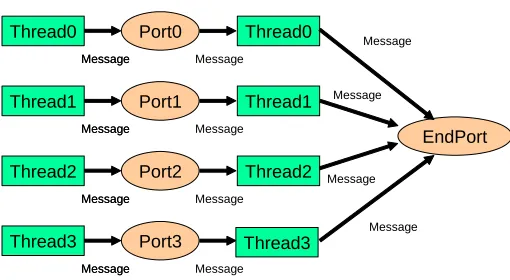
represents the class for which MPI is designed and where it gets its most stringent performance tests. Figure 1(a) illustrates a very simple loosely synchronous scenario showing threads posting and receiving messages through CCR ports.

As mentioned already, MPI has a rich set of defined methods that describe different synchronicity options, various utilities and a set of so-called collectives. These include the multi-cast (broadcast, gather-scatter) of messages with the calculation of associative and commutative functions on the fly. However as our target is today’s multi-core computers, the subtleties of the MPI collectives will not be relevant as one will not need

sophisticated implementations to get good performance on collectives for a few (4 in our tests) cores. Thus we concentrate on the equivalent of MPI send-receive tests. Posting to a port in CCR corresponds to a MPISEND and the matching MPIRECV is achieved from arguments of handler invoked to process port.

Message

Thread0 Port0

Message

Message Message

Thread0 Port0

Message

Message Message

Thread0 Port0

Message Message

Message

Thread3 Port3

Message

Message Message

Thread3 Port3

Message

Message Message

Thread3 Port3

Message Message

Message

Thread2 Port2

Message

Message Message

Thread2 Port2

Message

Message Message

Thread2 Port2

Message Message

Message

Thread1 Port1

Message

Message Message

Thread1 Port1

Message

Message Message

Thread1 Port1

Message Message

One Stage

Fig. 1(a) Idealized loosely synchronous execution in CCR

2. Performance of CCR as an MPI Engine

Our first set of tests used

the CCR Interleave

paradigm combining multiple stages of the type illustrated in figure 1(a) with a final collective shown in figure 1(b). This is characteristic of the simple MPI routines where

for example decompositions in one

dimension would lead the message structure of figures 1(c) and 1(d) for periodic or fixed end-points respectively. The patterns of figures 1(c) and 1(d) would lead to similar performance to the case of figure 1(a) as discussed in section 2. Note figure 1(d) is not trivially supported by today’s CCR as the ports need to be triggered by different number of messages. We will discuss such issues later in section 4. We choose a basic calculation for each stage that is a

Message

Thread0 Port0

Message Message

Thread0

Message

Message

Thread3 Port3

Message Message

Thread3

EndPort

Message

Thread2 Port2

Message Message

Message Thread2 _Message Message

Thread1 Port1

Message Message

Thread1 Message

multiple of a simple series computation that takes approximately 1.4 microseconds when

run on its own on a single core. We choose this size as the hardest loosely synchronous problems execute for around this time in each stage and require MPI latencies in the microsecond range. Of course one can in most technical problems increase the average compute time (or rather the compute-communication ratio) by increasing the grain size assigned to each core but our choice seems appropriate.

Write Exchanged Messages

Port3 Port2

Thread0

Thread3 Thread2 Thread1 Port1

Port0 Thread0

Write Exchanged Messages

Port3

Thread2 _Port2

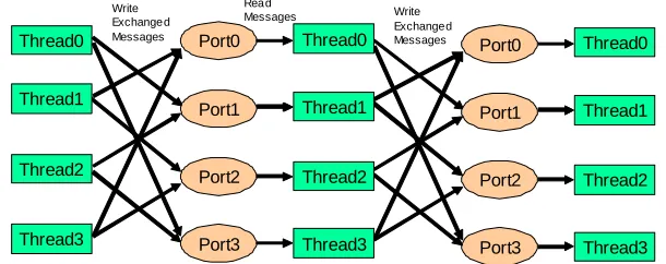
Fig. 1(c) Exchanging Messages with 1D Torus Exchange topology for loosely synchronous execution in CCR

Thread0

Read Messages

Thread3 Thread2 Thread1 Port1

Port0

Thread3 Thread1

Our initial experiments reported in figures 2-AMD to 6-AMD were performed on a Hewlett-Packard (HP) xw9300 workstation with 4 gigabytes of memory and two AMD Opteron chips – each with two cores. Each processor runs at 2.19 GHz speed. Further results in figures 2-Intel to 6-Intel were obtained from a Dell Precision Workstation 670 with two dual-Core Intel® Xeon™ Processor running at 2.80GHz with 2x2MB L2 cache. The system had 8 gigabytes of total memory. The Intel machine is about 7% slower in computation than the AMD PC in our tests and we will discuss the CCR performance for the two machines below. In a nutshell, the AMD shows better thread performance while the Intel machine usually has better memory bandwidth for message data exchange. We needed to disable the audio subsystem on the Dell PC as well as a few windows services such as “Automatic Updates”. We also needed to reboot the computer in between significant test runs to avoid downgraded performance due to problems like memory leak. By cleaning up the computer, we maintained a consistent testing environment thus obtained stable performance results between executions. Both machines run Windows XP Professional (64 bit edition) version 2003 and our code is written in C# with the CCR runtime (Ccr.Core.dll) downloaded from Microsoft Robotics Studio [Robotics] using June 2006 release.

Thread0

Write Exchanged Messages

Port3

Thread2 _Port2

Fig. 1(d) Exchanging Messages with 1D Exchange topology for loosely synchronous execution in CCR

Thread0

Read Messages

Thread3 Thread2 Thread1 Port1

Port0

In figure 2-AMD and 2-Intel, we plot the total execution time for a series of computations. Each ran 4.107 repetitions of the basic 1.4 microsecond compute activity (it is this long on AMD, it is 1.5 microsecond on Intel) on 4 cores. The repetitions are achieved by either a simple loop of basic computation unit or by splitting into stages

separated by writing and reading CCR ports. This simple strategy ensures that without threading overhead the execution time will be identical however one divides computation by loops or CCR stages; this way we can get accurate estimates of the overhead incurred by the port messaging interface.

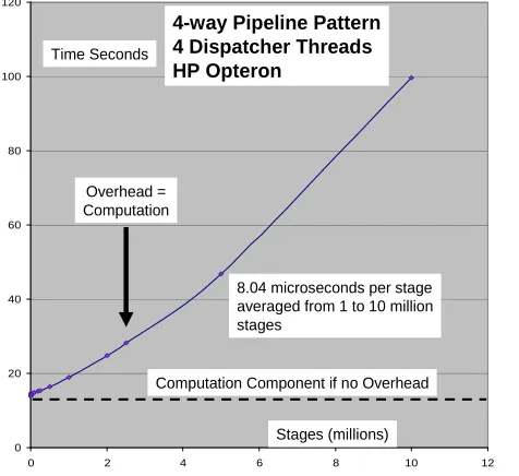
We first analyze the AMD results where without overhead the execution time will be about 14 seconds and is shown as a dashed line in figure 2-AMD. The figure takes these 4.107 repetitions and plots their execution time when divided into stages of the type shown in figure 1(a). Each measurement was an average over at least 10 runs with a given set of parameters. Figure 2 shows the results plotted up to 10 million stages while figure 3 shows the detail for up to one million stages. Always we use the term overhead to represent the actual measured execution time with subtraction of the time that a single stage would take to execute the same computational load. Figure 2

marks as “overhead=computation”, the

point where measured execution time is twice that taken by a single stage. For 10 million stages the overhead on the AMD is large – almost 85 seconds; this corresponds to a set of loosely synchronous stages lasting 9.9 microseconds which is mainly overhead as the

0 20 40 60 80 100 120 140 160

0 2 4 6 8 10 12

Stages (millions)

Fig. 2-Intel: Fixed amount of computation (4.107_{units) divided} into 4 cores and from 1 to 107_{stages on Dell Xeon Multicore. Each} stage separated by reading and writing CCR ports in Pipeline mode

Time Seconds

12.40 microseconds per stage averaged from 1 to 10 million stages

4-way Pipeline Pattern 4 Dispatcher Threads Dell Xeon

Overhead = Computation

Computation Component if no Overhead

0 20 40 60 80 100 120

0 2 4 6 8 10 12

Stages (millions)

Fig. 2-AMD: Fixed amount of computation (4.107_{units) divided into} 4 cores and from 1 to 107_{stages on HP Opteron Multicore. Each} stage separated by reading and writing CCR ports in Pipeline mode

Time Seconds

8.04 microseconds per stage averaged from 1 to 10 million stages

Overhead = Computation

Computation Component if no Overhead

“real” computation is just 1.4 microseconds per stage. The Intel results show 125 seconds overhead in this extreme case.

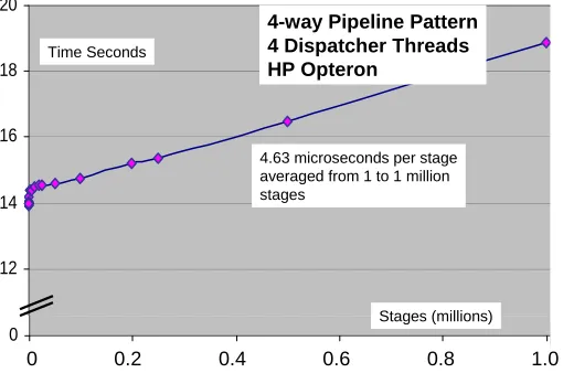
Looking at the case of one million stages, the overhead is much smaller – about 5 seconds (for AMD and 9 seconds for Intel); for the AMD, this corresponds to a set of loosely synchronous stages lasting 19 microseconds where the overhead is about 5 microseconds and the “real” computation is 14 microseconds (a loop of ten basic computation unit) per stage. Linear fits to the stage dependence leads to an overhead per stage of 4.63 microseconds from figure 3-AMD while the behavior becomes clearly

nonlinear in the larger range of stages in figure 2. This overhead represents the CCR (and system) time to set up threads and process the ports. Our measurement says this overhead is linear in the number of invocations when the spawned threads execute for substantially more (14 microseconds) than the basic overhead (4.63 microseconds) but the overhead increases when the thread execution time decreases to a few microseconds. Presumably CCR can be optimized and so we don’t read much into this observation at this stage; it needs more investigation. Turning to the Intel results they are qualitatively similar but with significantly higher overhead. In figure 2-Intel, the average has increased from 8.04 for AMD to 12.66 microseconds with the execution of 10 million stages taking 40% longer than the AMD even though the performance with 1 stage is only 7% longer. Comparing figure AMD and 3-Intel, shows the discrepancy between AMD and Intel CCR performance to be exacerbated if one restricts attention to just the first one million stages.

10 12 14 16 18 20

10 12 14 16 18 20

0 0

4-way Pipeline Pattern 4 Dispatcher Threads HP Opteron

Time Seconds

4.63 microseconds per stage averaged from 1 to 1 million stages

Stages (millions)

0 0.2 0.4 0.6 0.8 1.0

Fig. 3-AMD: Detail from Fig.2-AMD for 1 to 1 million stages on HP Opteron Multicore

14 15 16 17 18 19 20 21 22 23

24 4-way Pipeline Pattern 4 Dispatcher threads Dell Xeon

Time Seconds

9.25 microseconds per stage averaged from 1 to 1 million stages

Stages (millions)

0 0.2 0.4 0.6 0.8 1.0

We also need to examine the assignment of threads to cores. We did not have access to an Intel thread debugger for C# but the AMD thread debugger showed this to be efficient for small number of stages with each thread running on a different core. It is not clear what the interaction between port handler threads (the “real” computation) and the CCR

system processing shows on the timescale of microseconds. We investigated this a little in a “scaling” test that compared the results above with a similar set of runs that used fewer ports (and associated computations) than the 4 ports and threads in figures 2 and 3. In particular we look in figures 4 and 5 at just two ports leaving the remaining two “free” for other work if CCR and/or the system could make good use of them. These figures analogously to figures 2 and 3, show up to 10 million and up to one million stages with separate AMD and Intel measurements. These figures demonstrate that using just 2 cores in CCR showed substantial reduction in overhead with a more nearly linear dependence on the number of stages. The latency per stage for the AMD machine drops from 8.04 to

Fig. 4-AMD: Fixed amount of computation (2.107_units)

divided into 2 cores and from 1 to 107_{stages on HP}

Opteron Multicore. Each stage separated by reading and writing CCR ports in Pipeline mode.

0 5 10 15 20 25 30 35 40 45 50

0 2 4 6 8 10

Time Seconds

Stages (millions) 3.17 microseconds per stage averaged from 1 to 10 million stages

2-way Pipeline Pattern 2 Dispatcher Threads HP Opteron

0 10 20 30 40 50 60

0 2 4 6 8 10

Fig. 4-Intel: Fixed amount of computation (2.107_units) divided into 2 cores and from 1 to 107_{stages on Dell} Xeon Multi-core. Each stage separated by reading and writing CCR ports in Pipeline mode.

Stages (millions) 4.20 microseconds per stage averaged from 1 to 10 million stages

Time Seconds

2-way Pipeline Pattern 2 Dispatcher Threads Dell Xeon

13.5 14 14.5 15 15.5 16 16.5 17

Time Seconds

Stages (millions)

0 0.2 0.4 0.6 0.8 1.0

Fig. 5-AMD: Detail from Fig.4 for 0 to 1 million stages on HP Opteron Multicore

14 15 16 17 18 19

2-way Pipeline Pattern 2 Dispatcher Threads Dell Xeon

2-way Pipeline Pattern 2 Dispatcher Threads HP Opteron

Time Seconds

2.63 microseconds per stage averaged from 1 to 1 million

stages 3.39 microseconds per stage

averaged from 1 to 1 million stages

Stages (millions)

0 0.2 0.4 0.6 0.8 1.0

3.17 microseconds averaged over 10 million stages and from 4.63 to 2.63 microseconds when averaged from a single to one million stages. The Intel results shown in figure 4-Intel show even bigger improvements; the latency per stage drops from 12.40 to 4.20 microseconds averaged over 10 million stages and from 9.25 to 3.39 microseconds when averaged from a single to one million stages. We were surprised by this reduced latency, as for say 2 computation threads (ports) and 2 CCR cores, the debugger suggests that all the work (whether computation or overhead) is done on two threads and two cores are essentially idle. This observation makes it difficult to understand why the overhead is

smaller in this case than when more computation threads are used as there appear to be idle cores available for use without increasing overhead. As technology advances and the number of cores per chip increases, it will be important to investigate how many CCR threads would be best to use. As discussed later, the performance does depend on a “technical” parameter in CCR – namely the number of threads to be created by the dispatcher; the results in figures 2 to 5 specify 4 CCR dispatcher threads for the 4-way and 2 CCR dispatcher threads for the 2-way case. As shown later in tables 1 and 2, the latter choice gives better performance for 2-way computations than the CCR default which we believe is 4 threads.

0 20 40 60 80 100 120 140

0 1 2 3 4 5

Stages (millions) 20.9 microseconds per stage averaged from 1 to 5 million stage Time Seconds

Fig. 6-AMD: Fixed amount of computation (4.107_units) divided into 4 cores and from 1 to 107_{stages on HP Opteron} Multicore. Each stage separated by reading and writing CCR ports in Exchange mode

4-way Exchange Pattern 2 Dispatcher Threads HP Opteron

Fig. 6-Intel: Fixed amount of computation (4.107_{units) divided} into 4 cores and from 1 to 107_{stages on Dell Xeon multicore.} Each stage separated by reading and writing CCR ports in Exchange mode

0 50 100 150 200 250 300 350 400 450

0 2 4 6 8 10

Stages (millions) 40.4 microseconds per stage averaged from 1 to 10 million stage Time Seconds

4-way Exchange Pattern 4 Dispatcher Threads Dell Xeon

The results so far have used the pipeline pattern of figure 1(a) which captures the key loosely synchronous character of the MPI programming model but is not a very interesting messaging pattern as the threads send messages to themselves. The patterns of figure 1(c) and 1(d) are typical of MPI messaging used in data decomposition problems as it is that required by local communications with a one dimensional topology. Figure 6 corresponds to the scenario of figures 2 and 3 but with the Exchange pattern replacing the Pipeline. The stage overhead is substantially higher (20.9 and 40.4 microseconds for AMD and Intel respectively) and illustrate again that the underperformance of the Intel chip is increased by more complex operations. We tried to clarify this by looking at a broader set of other configurations.

each stage. We also show in tables 1,2-INTEL8, recent results for a Dell PWS-690 Precision workstation with two 4-core Intel® Xeon™ processors; note that the per core timing of the basic unit has increased from 30 microseconds per stage on Intel dual core two processor Xeon to 34 microseconds. Remember the AMD machine has 28 microsecond stage performance. The 8-core Dell machine has a total of 8 gigabytes of memory and runs the same Windows XP professional 84 bit edition. Each of the 8 cores runs at a slower 1.86 Ghz compared to 2.8 Ghz of Dell 4 core machine which explains decreased performance per core on the 8 core compared to 4 core Dell. We also used updated CCR software for just the INTEL8 tables which use the December 2006 CCR release.

Thread0

Port3

Thread2 Port2

Port1 Port0

Thread3 Thread1

Thread2 Port2

Thread0 Port0

Port3 Thread3

Port1 Thread1

Thread3 Port3 Thread2 Port2 Thread0 Port0

Thread1 Port1

(a) Pipeline (b) Shift

(d) Exchange

Thread0

Port3

Thread2 Port2

Port1 Port0

Thread3 Thread1

(c) Two Shifts

Fig. 7: Four Communication Patterns used in Tables 1 and 2. (a) and (b) use CCR Receive while (c) and (d) use CCR Multiple Item Receive

where each thread sends two messages to the same port. This should be identical to Shift (as messages are essentially zero size here) and the much larger overheads for “Two Shift” compared to Shift suggests that differences in the CCR software modules accounts for some of the increased overhead of Exchange compared to Pipeline and Shift. We assume it would be straightforward to improve the performance of Exchange.

We also note the reasonable performance on the 4-core AMD and Intel machines of Pipeline and Shift for 8-way parallel computations with about double the overhead compared to 4-way. Such a doubling is not implausible but we need to understand it better. Reasonable support of 8-way computations is important as one wants to support cases where the program uses more logical processors than the concurrent machine’s number of physical cores.

As mentioned earlier the default thread setting for CCR is usually not optimal when one runs fewer computations than cores. Having “spare” cores for 1 2 and 3 way parallelism clearly decreases the overhead but one still gets more computation done by using 4 or 8 way parallelism. We note that for Exchange we sometimes got errors (non terminating programs) which we are investigating further. MultipleItemReceive in CCR did not seem to work for just one item and so we could not directly compare it with Receive. Actually the semantics of MultipleItemReceive are not correct for Exchange as MPI requires not just two messages in Exchange but rather two messages from particular sources. We could use more precisely MultiplePortReceive but this is perhaps problematical in general as it requires one port for each pair of threads – an architecture that doesn’t scale as it needs N2 ports for N cores. We didn’t investigate further as it seems likely one should develop specialized CCR primitives for CCR if one wishes to fully support MPI from CCR.

Turning to the 8-core results in tables 1, 2-INTEL8, we find similar conclusions with significantly lower overheads except for the double shift case. The overhead for 8-way patterns on the 8-core machine is lower than that for 4-way patterns on the 4-core machine. As the 8-core machine has slower cores, the overhead is even lower if expressed as a percentage of computation time. We did find occasional errors as reported in earlier tables but we reran jobs and quoted results from averaging correct runs. We need to investigate if some of changes in results come from using updated CCR software as the AMD and INTEL tables use the June 2006 release and INTEL8 that from December 2006. Note the default to use 8 dispatcher threads again always performs more poorly than matching dispatcher threads to simultaneous computations except of course for the full 8-way case. It is curious that default overhead is typically higher on n<8 way parallelism than on 8 way case. The extra cores slow down the system!

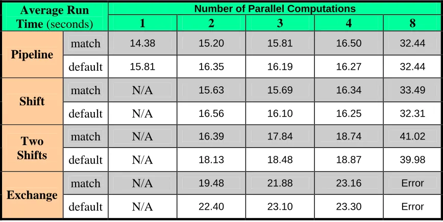
Table 1-AMD: Run times in seconds for the four patterns illustrated in Figure 7

Number of Parallel Computations

Average Run

Time (seconds) 1 2 3 4 8

match 14.38 15.20 15.81 16.50 32.44

Pipeline

default 15.81 16.35 16.19 16.27 32.44

match N/A 15.63 15.69 16.34 33.49

Shift

default N/A 16.56 16.10 16.25 32.31

match N/A 16.39 17.84 18.74 41.02

Two

Shifts _{default N/A 18.13 18.48 18.87 39.98}

match N/A 19.48 21.88 23.16 Error

Exchange

default N/A 22.40 23.10 23.30 Error

Match implies dispatcher thread number set to number of parallel computations; default implies thread number defaulted. Each run executed on 4 core Opteron-based PC and used 500,000 stages

Table 2-AMD: Stage overheads in microseconds for the four patterns illustrated in Figure 7 and calculated from the 500,000 stage runtimes of Table1 -AMD

Number of Parallel Computations

Stage Overhead

(microseconds) 1 2 3 4 8

match 0.77 2.4 3.6 5.0 8.9

Straight Pipeline

default 3.6 4.7 4.4 4.5 8.9

match N/A 3.3 3.4 4.7 11.0

Shift

default N/A 5.1 4.2 4.5 8.6

match N/A 4.8 7.7 9.5 26.0

Two

Shifts _{default N/A 8.3 9.0 9.7 24.0}

match N/A 11.0 15.8 18.3 Error

Exchange

default N/A 16.8 18.2 18.6 Error

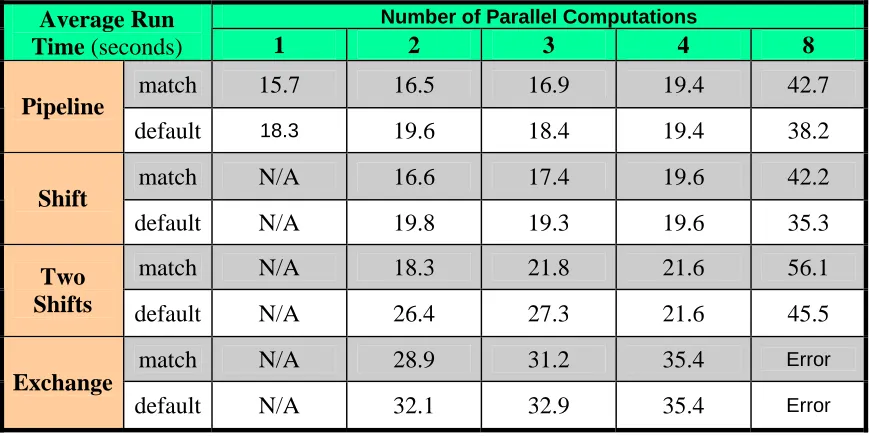
Table 1-INTEL: Run times in seconds for the four patterns illustrated in Figure 7

Number of Parallel Computations

Average Run

Time (seconds) 1 2 3 4 8

match 15.7 16.5 16.9 19.4 42.7

Pipeline

default 18.3 19.6 18.4 19.4 38.2

match N/A 16.6 17.4 19.6 42.2

Shift

default N/A 19.8 19.3 19.6 35.3

match N/A 18.3 21.8 21.6 56.1

Two

Shifts _{default N/A 26.4 27.3 21.6 45.5}

match N/A 28.9 31.2 35.4 Error

Exchange

default N/A 32.1 32.9 35.4 Error

Match implies dispatcher thread number set to number of parallel computations; default implies thread number defaulted. Each run executed on 4 core Xeon-based Dell PC and used 500,000 stages

Table 2-INTEL: Stage overheads in microseconds for the four patterns illustrated in Figure 7 and calculated from the 500,000 stage runtimes of Table 1-INTEL

Number of Parallel Computations

Stage Overhead

(microseconds) 1 2 3 4 8

match _(0.77)1.7 _(2.4)3.3 _(3.6)4.0 _(5.0)9.1 25.9 _(8.9)

Straight Pipeline

default _(3.6) 6.9 _(4.7)9.5 _(4.4)7.0 _(4.5) 9.1 16.9 _(8.9)

match N/A _(3.3)3.4 _(3.4)5.1 _(4.7)9.4 _(11.0)25.0

Shift

default N/A _(5.1)9.8 _(4.2)8.9 _(4.5)9.4 11.2 _(8.6)

match N/A 6.8

(4.8)

13.8 (7.7)

13.4 (9.5)

52.7 (26.0) Two

Shifts _{default N/A} 23.1 (8.3)

24.9 (9.0)

13.4 (9.7)

31.5 (24.0)

match N/A _(11.0)28.0 _(15.8)32.7 _(18.3)41.0 Error

Exchange

default N/A _(16.8)34.6 _(18.2)36.1 _(18.6)41.0 Error

Table 1-INTEL8: Run times in seconds for the four patterns illustrated in Figure 7

Number of Parallel Computations

Average Run

Time (seconds) 1 2 3 4 8

match 17.6 19.1 19.1 19.3 20.2

Pipeline

default 20.1 21.2 21.8 21.7 20.2

match N/A 19.1 19.2 19.5 20.6

Shift

default N/A 21.1 22.1 22.0 20.6

match N/A 20.7 20.4 21.2 28.4

Two

Shifts _{default N/A 27.1 32.2 30.6 28.4}

match N/A 30.3 28.7 27.6 33.5

Exchange

default N/A 32.6 36.3 40.0 33.7

Match implies dispatcher thread number set to number of parallel computations; default implies thread number defaulted. Each run executed on 8 core Xeon-based Dell PC and used 500,000 stages

Table 2-INTEL8: Stage overheads in microseconds for the four patterns illustrated in Figure 7 and calculated from the 500,000 stage runtimes of Table 1-INTEL8

Number of Parallel Computations

Stage Overhead

(microseconds) 1 2 3 4 8

match _(1.7)1.33 _(3.3)4.2 _(4.0)4.3 _(9.1)4.7 _(25.9)6.5

Straight Pipeline

default _(6.9) 6.3 _(9.5)8.4 _(7.0)9.8 _(9.1) 9.5 _(16.9)6.5

match N/A _(3.4)4.3 _(5.1)4.5 _(9.4)5.1 _(25.0)7.2

Shift

default N/A _(9.8)8.3 _(8.9)10.2 _(9.4)10.0 _(11.2)7.2

match N/A 7.5

(6.8)

6.8 (13.8)

8.4 (13.4)

22.8 (52.7) Two

Shifts _{default N/A} 20.3 (23.1)

30.4 (24.9)

27.3 (13.4)

23.0 (31.5)

match N/A _(28.0)26.6 _(32.7)23.6 _(41.0)21.4 _(error) 33.1

Exchange

default N/A _(34.6)31.3 _(36.1)38.7 _(41.0)46.0 33.5

3. CCR MPI Bandwidth

0 50 100 150 200 250 300 350 400

0 2 4 6 8 10

Fig. 8-Intel: Scenario from Fig.2-Intel with run time plotted versus number of stages with 1000 words of double array copied in each stage from thread in stepped

locations in a large array on Dell Xeon Multicore

Time Seconds

Total Bandwidth 1.56 Gigabytes/Sec

4-way Pipeline Pattern 4 Dispatcher Threads Dell Xeon

Stages (millions)

Fig. 8-AMD: Scenario from Fig.2-AMD with run time plotted versus number of stages with 1000 words of double array copied in each stage from thread to stepped locations in a large array on HP Opteron Multicore.

Time Seconds

Total Bandwidth 1.29 Gigabytes/Sec

Stages (millions)

0 2 4 6 8 10

50 100

0 200 300 400

4-way Pipeline Pattern 4 Dispatcher Threads HP Opteron

0 200 400 600 800 1000 1200 1400 1600

0 2 4 6 8 10

To measure MPI bandwidth, we simulated a typical MPI CALL such as subroutine

mpisend (buf, count, datatype, dest, tag, comm) by posting a structure made up of an array of doubles of length N and a set of six integers (with one extra integer for CCR control). These all used the full 4-way parallelism and the results are shown in figures 8 to 12. One passes a reference for the data buffer buf and we used three distinct models for locations of final data termed respectively

a) Inside Thread: The buffer buf is copied using C# Copy To function to a new array inside the thread whose size is identical to that of buf.

Fig. 9-AMD: Scenario from Fig.2-AMD for 5,000 stages with run time plotted against size of double array copied in each stage from thread to stepped locations in a large array on HP Opteron Multicore.

Total Bandwidth 1.15 Gigabytes/Sec up to one million double words and 1.19 Gigabytes/Sec up to 100,000 double words Time Seconds

Array Size: Millions of Double Words 0 20 40 60 80 100 120 140 160 180 200

0 0.2 0.4 0.6 0.8 1

4-way Pipeline Pattern 4 Dispatcher Threads Dell Xeon

4-way Pipeline Pattern 4 Dispatcher Threads HP Opteron

Time Seconds

Total Bandwidth 1.0 Gigabytes/Sec up to one million double words and 1.75 Gigabytes/Sec up to 100,000 double words

Array Size: Millions of Double Words

b) Outside Thread: The buffer buf is copied using C# Copy To function to a fixed array (with distinct arrays for each core) outside the thread whose size is identical to that of buf.

c) Stepped Array Outside Thread: The buffer buf is copied using element by element Copy in C# to a fixed large array outside the thread whose size is two million double floating words. Again each core has its own separate stepped array.

Note all measurements in this section involved 4-way parallelism and the bandwidth is summed over all four cores simultaneously copying message buffers.

In figure 8, we repeat the measurements of figure 2 but add the transfer of 1000 double floating words (and the six integers) to each of the 4 ports at each stage. We see a nice linear dependence on the number of stages and estimate a total (over the 4 cores) bandwidth of about a 1.29 (AMD) and 1.56(Intel) Gigabytes/second corresponding to this transfer. This used the stepped array model c) defined above with each successive 1000 words stored in the next available space in an array (separate for each core) of total length of 20 million words. After 20,000 stages the array is full and one wraps back to the start. An MPI program could in fact just use pointers to the shared memory and not copy data between processes. However the explicit copying model used here is free of dependencies and typical of a simple safe concurrent MPI program. Interpretation of figure 8 is tricky as one is varying both amount of data and total stage overhead as you increase the number of stages; the bandwidth is extracted by subtracting the data used to make figures 2 and 8.

The bandwidth is better estimated from figures 9-12 which fix the number of stages and hence fix the CCR staging overhead. We look at the run time as a function of size of array stored in the port and summarize the results in table 3 (with separate AMD and Intel versions). One finds bandwidths that vary from 0.75 to 2 Gigabytes per second with the Intel machine claiming both upper and lower values although it typically shows better bandwidth than the AMD machine. Note the best bandwidths are obtained when the destination arrays are outside the thread and when of course the copied data is small enough to stay in cache. We used 100,000 words in the summary tables 1 and 2 to illustrate the “in cache” case and one or ten million for the “out of cache” case. Also the bandwidth higher for the cases where the computing component is significant; i.e. when it has a value of a few milliseconds rather than the lower limit of a few microseconds. Figure 9 illustrates this with a stage computation of 2800 (AMD) to 3000 (Intel) microseconds. For the case (c) of a stepped array, the Intel PC achieves a bandwidth of 1.75 gigabytes/second for 100,000 word messages which decreases to just 1 gigabyte/second for million word arrays. The AMD machine shows a roughly uniform bandwidth of 1.17 gigabyte/second independent of array size. Note typical messages in MPI would be smaller than 100,000 words and so MPI would benefit from the performance increase for small messages.

corresponds to a “small” (40 computation units per core per stage; taking 56 and 60 microseconds for AMD and Intel respectively) computation case. Now the stepped array bandwidth for Intel is lower in fig 10(c) than in figure 9 and we only see high Intel bandwidth in the case of figure 10(b); 100,000 words copied to an array outside the thread with same size as message. Note over the measurements reported from AMD in figure 10 the bandwidth varies from 0.89 to 1.16 gigabytes/second; the Intel numbers vary from 0.76 to 1.89 gigabytes/second. Given the stable AMD results, figures 11 and 12 only examine the Intel machine and repeat figures 10(a) and 10(b) with a 100 times longer computation (4000 units per core per stage). One always sees an improved bandwidth with over a factor of two improvements in the case of copying to an array inside the thread. For 100,000 words, the bandwidth goes from 0.83 gigabytes/second in figure 10(a) to 1.74 gigabytes/second in figure 11.

0 20 40 60 80 100 120

0 0.2 0.4 0.6 0.8 1

Fig. 10a-Intel: Fixed amount of computation (4.105_units) divided into 4 cores and 2,500 stages. Each stage separated by reading and writing CCR ports in Pipeline mode. Run time plotted against size of double array copied in each stage from thread to same size array inside thread on Dell Xeon Multicore

Time Seconds 0 100 200 300 400 500 600 700 800 900

0 2 4 6 8 10

4-way Pipeline Pattern 4 Dispatcher Threads HP Opteron

4-way Pipeline Pattern 4 Dispatcher Threads Dell Xeon

Time Seconds

Total Bandwidth 0.99 Gigabytes/Sec up to one million double words and 0.89 Gigabytes/Sec

up to 100,000 double words

Total Bandwidth 0.83 Gigabytes/Sec up to one million double words and 0.76 Gigabytes/Sec

up to 100,000 double words

Array Size: Millions of Double Words Array Size: Millions of Double Words

Fig. 10a-AMD: Fixed amount of computation (4.105 units) divided into 4 cores and 2,500 stages. Each stage separated by reading and writing CCR ports in Pipeline mode. Run time plotted against size of double array copied in each stage from thread to same size array inside thread on HP Opteron Multicore

0 100 200 300 400 500 600 700 800

0 2 4 6 8 10

Fig. 10b-AMD: Fixed amount of computation (4.105 units) divided into 4 cores and 2,500 stages. Each stage separated by reading and writing CCR ports in Pipeline mode. Run time plotted against size of double array copied in each stage from thread to same size array outside thread on HP Opteron Multicore

Time Seconds

4-way Pipeline Pattern 4 Dispatcher Threads HP Opteron

Total Bandwidth 1.11 Gigabytes/Sec up to one million double words and 1.16 Gigabytes/Sec

up to 100,000 double words

0 10 20 30 40 50 60 70 80 90 100

0 200 400 600 800 1000

4-way Pipeline Pattern 4 Dispatcher Threads Dell Xeon

Time Seconds

Total Bandwidth 0.89 Gigabytes/Sec up to one million double words and 1.89 Gigabytes/Sec

up to 100,000 double words

Array Size: Millions of Double Words

Array Size: Millions of Double Words

0 20 40 60 80 100 120

0 0.2 0.4 0.6 0.8 1

Fig. 11-Intel: Fixed amount of computation (4.107_{units) divided} into 4 cores and 2,500 stages. Each stage separated by reading and writing CCR ports in Pipeline mode. Run time plotted against size of double array copied in each stage from thread to same size array inside thread on Dell Xeon Multicore

Time Seconds

4-way Pipeline Pattern 4 Dispatcher Threads Dell Xeon

Total Bandwidth 0.9 Gigabytes/Sec up to one million double words and 1.74 Gigabytes/Sec

up to 100,000 double words

Array Size: Millions of Double Words 0 10 20 30 40 50 60 70 80 90 100

0 0.2 0.4 0.6 0.8 1

Fig. 12-Intel: Fixed amount of computation (4.107_{units) divided} into 4 cores and 2,500 stages. Each stage separated by reading and writing CCR ports in Pipeline mode. Run time plotted against size of double array copied in each stage from thread to same size array outside thread on Dell Xeon Multicore

Time Seconds

4-way Pipeline Pattern 4 Dispatcher Threads Dell Xeon

Total Bandwidth 1.07 Gigabytes/Sec up to one million double words and 2.0 Gigabytes/Sec

up to 100,000 double words

Array Size: Millions of Double Words

0 100 200 300 400 500 600 700 800

0 2 4 6 8 10

Fig. 10c-AMD: Fixed amount of computation (4.105 units) divided into 4 cores and 2,500 stages. Each stage separated by reading and writing CCR ports in Pipeline mode. Run time plotted against size of double array copied in each stage from thread to stepped locations in a large array on HP Opteron Multicore

Time Seconds

4-way Pipeline Pattern 4 Dispatcher Threads HP Opteron

Total Bandwidth 1.14 Gigabytes/Sec up to one million double words and 1.13 Gigabytes/Sec

up to 100,000 double words

Array Size: Millions of Double Words

Fig. 10c-Intel: Fixed amount of computation (4.105_{units) divided} into 4 cores and 2,500 stages. Each stage separated by reading and writing CCR ports in Pipeline mode. Run time plotted against size of double array copied in each stage from thread to stepped locations in a large array on Dell Xeon Multicore

0 10 20 30 40 50 60 70 80 90 100

0 0.2 0.4 0.6 0.8 1

Time Seconds

4-way Pipeline Pattern 4 Dispatcher Threads Dell Xeon

Total Bandwidth 0.89 Gigabytes/Sec up to one million double words and 1.16 Gigabytes/Sec

up to 100,000 double words

Table 3-AMD: Measured total bandwidths summed over all four cores for 3 different array locations described in the text

Bandwidths in Gigabytes/second summed over 4 cores

Array Inside Thread Array Outside

Threads

Stepped Array Outside Thread Number of

stages

Small Large Small Large Small Large

Approx. Compute Time per stage µs

250000 0.90 0.96 1.08 1.09 1.14 1.10 56.0

0.89 0.99 1.16 1.11 1.14 1.13 2500

Fig 10a Fig 10b

1.13 up to 107 words Fig 10c

56.0

1.19 1.15 5000

Fig 9 2800

1.15 1.13 200000

1.13 up to 107 words 70

Each stage executed a computational task after copying data arrays of size 105 (labeled small), 106 (labeled large) or 107 double words. The last column is an approximate value in microseconds of the compute time for each stage. Note that copying 100,000 double precision words per core at a gigabyte/second bandwidth takes 3200 µs. The data to be copied (message payload in CCR) is fixed and its creation time is outside timed process.

Table 3-Intel: Measured total bandwidths summed over all four cores for 3 different array locations described in the text

Bandwidths in Gigabytes/second summed over 4 cores

Array Inside Thread Array Outside

Threads

Stepped Array Outside Thread Number of

stages

Small Large Small Large Small Large

Approx. Compute Time per stage µs

250000 0.84 0.75 1.92 0.90 1.18 0.90 59.5

200000 1.21 0.91 74.4

1.75 1.0 5000

Fig 9 2970

0.83 0.76 1.89 0.89 1.16 0.89 2500

Fig 10a Fig 10b Fig 10c

59.5

1.74 0.9 2.0 1.07 2500

Fig 11 Fig 12

1.78 1.06 5950

4. Initial Performance Results on DSS

Fig. 13(a): Timing of HP Opteron Multicore as a function of number of two-way service messages processed (November 2006 DSS Release)

0 50 100 150 200 250 300 350

1 10 100 1000 10000

A v e ra ge r un t im e ( m ic ros e c onds )

Fig. 13(a): Timing of HP Opteron Multicore as a function of number of two-way service messages processed (November 2006 DSS Release)

0 50 100 150 200 250 300 350

1 10 100 1000 10000

A v e ra ge r un t im e ( m ic ros e c onds )

The Robotics release [Robotics] includes a lightweight service environment DSS for which we performed an initial evaluation on the AMD Opteron two processor two core machine. This analysis used the current November 2006 CCR/DSS software; note the CCR analysis discussed earlier used the June 2006 software release. In figure 13, we time groups of request-response two way messages running on (different) cores of the HP Opteron 4-core system. For a group of 200 messages we histogram the timings of 30 separate measurements. For low message counts DSS initialization bumps up the run time and for large groups of messages it increases – perhaps due to overheads like Garbage Collection. For message groups from about 50-1000 messages, we find average times of 40-50 microseconds or throughputs of 20,000 to 25,000 two-way messages per second. 0 10 20 30 40 50 60 70

0 500 1000 1500 2000 2500 3000 3500

Messages per Second

R ound Tr ip Ti m e ( m s) (

Grid Farm Sun Fire - 6 Cores Sun Fire - 8 Cores HP xw9300 Dell Intel Xeon

2 Chips 2 Core/chip “Gridfarm” 2 “old” Intel Chips 1 Core/chip

1 Sun Chip 8 Core/chip 1 Sun Chip

6 Core/chip

Xeon

Opteron

This result of internal service to internal service can be compared with the recent Apache

to

ice Axis 2 release where the performance of several multi-core computers is investigated. The same Opteron machine used in CCR/DSS analysis supports about 3,000 messages per second throughput. Figure 13 and 14 are not fair comparisons. Figure 13 is internal one machine so each service end-point has effectively just two cores. Figure 14 is external clients interacting on a LAN so there is network overhead but now the serv can access the full 4 cores. We will complete fairer comparisons later and also examine the important one-way messaging case.

(d) Rendezvous with Active Messages

Thread2 Port0

Thread0

Port1

Thread1 Thread3 Port0

(c) Rendezvous

Thread0 Recv Send

Thread1 Recv

Thread0 (b) Queued

Send

Thread1 Queue

Thread0 Thread2

Thread3 Port1

Port0

Thread1 (a) Spawned

(e) Publish-Subscribe Messaging

Thread1

Thread0

Thread1

Thread2

Thread3 (f) Overlay Network

Fig. 15: Structure of 6 messaging models

Thread2

Thread0 Topic0

= Port0

Thread3

5. Conclusions and Futures

his preliminary study suggests that CCR is an interesting infrastructure for parallel

figure 15, we compare six programming models with 15(a) showing CCR’s natural

Table 4: Classes of Parallel or Concurrent Messaging Systems

T

computing. We addressed this by showing it can support the basic loosely synchronous structure of most highly parallel technical computing problems. We may be off the mark but we see the problem is not “just” producing another MPI but more interestingly of designing message-based runtimes that support a variety of programming model that includes those used in technical computing but also those that might support concurrent programming for the broad range of applications that will use multicore architectures.

In

implementation of MPI style runtime. Note this model where threads are initiated to process messages is different from the conventional MPI model where persistent threads communicate with messages via rendezvous as seen in figure 15(c) or 15(d). In figure 15(c) we represent a common high performance MPI implementation where messages are transmitted between running processes and no extra threads are used. In figure 15(d), we insert a handler for each message as is used in active messages; this strategy is also common where for efficiency one uses the network hardware to handle external MPI messages – of course the processor on a network card can be considered as an extra core available to support message processing. We believe the model of figure 15(a) can be used for current MPI programs but some programming changes will be needed; one may be able to automate this change. The model of fig. 15(a) would be best supported by optimizing relevant CCR core modules and extending those currently available so that for example cases like figure 1(d) with differing number of messages in each port can be handled. This is interesting research but out of scope in this study. One must also look at the implementation of MPI and distributed programming involving both internal and external processes with conventional external messages arriving from MPICH and openMPI.

Messaging Model Software Typical Applications

Spawned (fig. 15(a))

Streamed dataflow; SOA

CCA, CCR, DSS Apache Synapse, Grid Workflow

Dataflow as in AVS, Image Processing; Grids; Web Services

Spawned

(fig. 15(a)) Tree Search CCR Optimization; Computer Chess

Queued (fig. 15(b))

Discrete Event

simulations openRTI, CERTI

Ordered Transactions; “war game” style simulations

Rendezvous (figs. 15(c, d))

Message Parallelism MPI

openMPI MPICH2

Loosely Synchronous applications including

engineering & science; rendering Publish-Subscribe

(fig. 15(e)) Enterprise Service Bus

NaradaBrokering Mule, JMS

Content Delivery;

Message Oriented Middleware

Overlay Networks

(fig. 15(f)) Peer-to-Peer

Jabber, JXTA,

As an alternative to adapting MPI to the implementation style of fig. 15(a), one could

EFERENCES

tnam Singh and Georgio Chrysanthakopoulos, “An Asynchronous ted instead produce a messaging system that supported multiple paradigms and allowed their integration in complex applications. Table 4 summaries some paradigms and typical applications. Other interesting messaging models are shown in the other parts of figure 15. Figure 15(b) shows a variant of the Rendezvous (figures 15(c, d)) where messages are queued in the destination process (thread). Figure 15(e) illustrates that classic publish-subscribe messaging models can also be supported by the ports underlying CCR’s model. Figure 15(f) shows another well known distributed messaging model; an overlay network as used in P2P systems. We expect to return this general messaging analysis later in our work after we have looked in more detail at the service infrastructure DSS built on top of CCR. Here we will also comment on Grid applications of CCR and multicore systems.

R

1. [CCR1] Sa

Messaging Library for C#”, Synchronization and Concurrency in Object-Orien Languages (SCOOL) at OOPSLA October 2005 Workshop, San Diego, CA.

http://urresearch.rochester.edu/handle/1802/2105 ()

2. [CCR2] “Concurrency Runtime: An Asynchronous Messaging Library for C#

rrencyRuntime

2.0” George Chrysanthakopoulos Channel9 Wiki Microsoft

http://channel9.msdn.com/wiki/default.aspx/Channel9.Concu

on

issues/06/09/ConcurrentAffairs/default.aspx

3. [CCR3] “Concurrent Affairs: Concurrent Affairs: Concurrency and Coordinati Runtime”, Jeffrey Richter Microsoft

http://msdn.microsoft.com/msdnmag/

005 4. [Graham05] Richard L. Graham and Timothy S. Woodall and Jeffrey M. Squyres

“Open MPI: A Flexible High Performance MPI”, Proceedings, 6th Annual International Conference on Parallel Processing and Applied Mathematics, 2

http://www.open-mpi.org/papers/ppam-2005

5. [MPI] Message passing Interface MPI Forum http://www.mpi-forum.org/index.html

6. [MPICH] MPICH2 implementation of the Message-Passing Interface (MPI)

http://www-unix.mcs.anl.gov/mpi/mpich/

7. [OpenMPI] High Performance MPI Message Passing Library http://www.open-

.K. Panda “How will we develop and program emerging robust, low-mpi.org/

8. [Panda06] D

power, adaptive multicore computing systems?” The Twelfth International Conference on Parallel and Distributed Systems ICPADS ‘06 July 2006 Minneapolis

http://www.icpads.umn.edu/powerpoint-slides/Panda-panel.pdf#search=%22mpi%20multicore%20performance%22

9. [PallasMPI] Thomas Bemmerl “Pallas MPI Benchmarks Results”

http://www.lfbs.rwth-aachen.de/content/index.php?ctl_pos=392

10.[Robotics] Microsoft Robotics Studio is a Windows-based environment that re. provides easy creation of robotics applications across a wide variety of hardwa It includes end-to-end Robotics Development Platform, lightweight service-oriented runtime, and a scalable and extensible platform. For details, see

11.[PCW] Fox, G. C., Messina, P., Williams, R., “Parallel Computing Works!”, Morgan Kaufmann, San Mateo Ca, 1994.

12.[PVMMPI] Geoffrey Fox Messaging Systems: Parallel Computing the Internet and the Grid EuroPVM/MPI 2003 Invited Talk September 30 2003

http://grids.ucs.indiana.edu/ptliupages/publications/gridmp_fox.pdf

13. [Source] “The Sourcebook of Parallel Computing” edited by Jack Dongarra, Ian Foster, Geoffrey Fox, William Gropp, Ken Kennedy, Linda Torczon, and Andy White, Morgan Kaufmann, November 2002.