Study on Parallel SVM Based on MapReduce

Study on Parallel SVM Based on MapReduce

Zhanquan Sun1,

Geoffrey Fox

Key Laboratory for Computer Network of Shandong Province, Shandong Computer Science Center, Jinan, Shandong, 250014, China

2

School of Informatics and Computing, Pervasive Technology Institute, Indiana University Bloomington, Bloomington, Indiana, 47408, USA

Abstract - Support Vector Machines (SVM) are powerful classification and regression tools. They have been widely studied by many scholars and applied in many kinds of practical fields. But their compute and storage requirements increase rapidly with the number of training vectors, putting many problems of practical interest out of their reach. For applying SVM to large scale data mining, parallel SVM are studied and some parallel SVM methods are proposed. Most currently parallel SVM methods are based on classical MPI model. It is not easy to be used in practical, especial to large scale data-intensive data mining problems. MapReduce is an efficient distribution computing model to process large scale data mining problems. Some MapReduce software were developed, such as Hadoop, Twister and so on. In this paper, parallel SVM based on iterative MapReduce model Twister is studied. The program flow is developed. The efficiency of the method is illustrated through analyzing practical problems.

Keywords: Parallel SVM, Large scale data, MapReduce, Twister

1

Introduction

With the development of electronic and computer technology, the quantity of electronic data is in exponential growth [1]. Data deluge has become a salient problem to be solved. Scientists are overwhelmed with the increasing amount of data processing needs arising from the storm of data that is flowing through virtually every science field, such as bioinformatics [2-3], biomedical [4-5], Cheminformatics [6], web [7] and so on. Then how to take full use of these large scale data to support decision is a big problem encountered by scientists. Data mining is the process of discovering new patterns from large data sets involving methods at the intersection of artificial intelligence, machine learning, statistics and database systems. It has been studied by many scholars in all kinds of application area for many years and many data mining methods have been developed and applied to practice. But most classical data mining methods out of reach in practice in face of big data. Computation and data intensive scientific data analyses are increasingly prevalent in recent years. Efficient parallel/concurrent algorithms and implementation techniques are the key to meeting the scalability and performance requirements entailed in such large scale data mining analyses. Many parallel algorithms are implemented using

different parallelization techniques such as threads, MPI, MapReduce, and mash-up or workflow technologies yielding different performance and usability characteristics [8]. MPI model is efficient in computation intensive problems, especially in simulation. But it is not easy to be used in practical. MapReduce is a cloud technology developed from the data analysis model of the information retrieval field. Several MapReduce architectures are developed now. The most famous is the Google, but the source code is not open. Hadoop is the most popular open source MapReduce software. It has been adopted by many huge IT companies, such as Yahoo, Facebook, eBay and so on. The MapReduce architecture in Hadoop doesn’t support iterative Map and Reduce tasks, which is required in many data mining algorithms. Professor Fox developed an iterative MapReduce architecture software Twister. It supports not only non-iterative MapReduce applications but also an non-iterative MapReduce programming model. The manner of Twister MapReduce is “configure once, and run many time” [9-10]. It can be applied on cloud platform. It will be the popular MapReduce architecture in cloud computing and can be used in data intensive data mining problems.

high-dimensional problems, remains to be seen. A parallelization scheme was proposed where the kernel matrix is approximated by a block-diagonal [17]. Most of parallel SVM are based on MPI programming model. Little research work has been done with MapReduce work.

Based on current research work of SVM and Twister MapReduce framework, the paper develops a parallel SVM model based on MapReduce. In this model, training samples are divided into subsections. Each subsection is trained with a SVM model. In this paper, libSVM is used to train each subSVM. The non-support vectors are filtered with subSVMs. The support vectors of each subSVM are taken as the input of next layer subSVM. The global SVM model will be obtained through iteration. The MapReduce based SVM model is encoded with Java language.

The following of the paper is organized as follows. LibSVM method is introduced briefly in part 2. The Twister model is introduced in part 3. MapReduce based parallel SVM model and its program flow is introduced in part 4. Two practical examples are analyzed with the proposed model in part 5. At last some conclusions are summarized.

2

LibSVM

2.1

Support Vector Machines

SVM first maps the input points into a high-dimensional feature space with a nonlinear mapping function and then carries through linear classification or regression in the dimensional feature space. The linear regression in high-dimension feature space corresponds to the nonlinear classification or regression in low-dimensional input space. The general SVM can be described as follows.

Let 𝑙 training samples be 𝑇= {(𝑥₁,𝑦₁),⋯, (𝑥_𝑙,𝑦_𝑙)}, where 𝑥_𝑖∈ 𝑅𝑛, 𝑦_𝑖∈{1,−1} (classification) or 𝑦_𝑖∈ 𝑅 (regression), 𝑖= 1,⋯,𝑙. Nonlinear mapping function is

𝑘�𝑥𝑖,𝑥𝑗�=∅(𝑥𝑖)∅�𝑥𝑗�. Classification SVM can be

implemented through solving the following equations.

min

𝑤,𝜉𝑖,𝑏� 1

2‖𝑤‖2+𝐶 � 𝜉𝑖

𝑖

�

𝑠.𝑡.𝑦𝑖_(Φ𝑇_(𝑋

𝑖)𝑤+𝑏)≥1− 𝜉𝑖 ∀𝑖= 1,⋯,𝑛 (1)

𝜉𝑖≥0 ∀𝑖= 1,⋯,𝑛

By introducing Lagrangian multipliers, the optimization problem can be transformed into its dual problem.

min

𝛼 � 𝛼𝑖𝛼𝑗𝑦𝑖𝑦𝑗𝑘(𝑥𝑖,𝑥𝑗) 𝑖,𝑗

− � 𝛼𝑖

𝑙

𝑖=1

𝑠.𝑡. 𝑦𝑇_{𝜶= 0 (2)}

0≤ 𝛼𝑖<𝐶,𝑖= 1,⋯,𝑙

After obtaining optimum solution 𝑎∗,𝑏∗, the following decision function is used to determine which class the sample belongs to.

𝑓(𝑥) =𝑠𝑔𝑛�∑ 𝑦𝑙𝑖=1 𝑖𝛼𝑖∗𝐾(𝑥𝑖,𝑥)+𝑏∗� (3)

The classification precision of the SVM model can be calculated as

Accuracy =#correctly predicted data_{#total testing data} × 100%

2.2

libSVM

LibSVM is taken as the most efficient SVM software. It is an integrated software for support vector classification, regression, and distribution estimation. Most efficient analysis models are included. For example, C-SVC and nu-SVC classification models, epsilon-SVR and nu-SVR regression models, and one-class SVM distribution estimation. For improving the classification correct rate, cross validation is adopted. For processing unbalancing classification problem, weighted and probability models are adopted. The detail of libSVM can be found in [12]. In this paper, C-SVC libSVM model is selected to analyze the classification problems.

3

Architecture of Twister

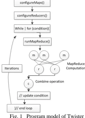
There are many parallel algorithms with simple iterative structures. Most of them can be found in the domains such as data clustering, dimension reduction, link analysis, machine learning, and computer vision. These algorithms can be implemented with iterative MapReduce computation. Professor Fox developed the first iterative MapReduce computation model Twister. It has several components, i.e. MapReduce main job, Map job, Reduce job, and combine job. Twister’s programming model can be described as in figure 1.

Fig. 1 Program model of Twister

MapReduce jobs are controlled by the client node through a multi-step process. During configuration, the client assigns MapReduce methods to the job, prepares KeyValue pairs and prepares static data for MapReduce tasks through the partition file if required. Between iterations, the client receives results collected by the Combine method, and, when the job is done, exits gracefully. The message communicate between job is realized with message brokers, i.e. NaradaBrokering or ActiveMQ.

scheduling for workers in order to take advantage of the local data cache. In this hybrid computing model, daemons communicate with the client through messages.

Reduce daemons operate on computation nodes. The number of reducers is prescribed in client configuration step. The reduce jobs depend on the computation results of Map jobs. The communication between daemons is through messages.

Combine job is to collect MapReduce results. It operates on client node. Twister uses scripts to operate on static input data and some output data on local disks in order to simulate some characteristics of distributed file systems. In these scripts, Twister parallel distributes static data to compute nodes and create partition file by invoking Java classes. For data which are output to the local disks, Twister uses scripts to gather data from all compute nodes on a single node specified by the user.

4

Parallel SVM based on Twister

4.1

Architecture of Parallel SVM

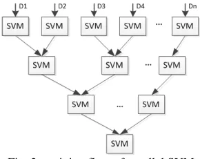
The parallel SVM is based on the cascade SVM model. The SVM training is realized through partial SVMs. Each subSVM is used as filter. This makes it straightforward to drive partial solutions towards the global optimum, while alternative techniques may optimize criteria that are not directly relevant for finding the global solution. Through the parallel SVM model, large scale data optimization problems can be divided into independent, smaller optimizations. The support vectors of the former subSVM are used as the input of later subSVMs. The subSVM can be combined into one final SVM in hierarchical fashion. The parallel SVM training process can be described as in figure 2.

Fig. 2 training flow of parallel SVM

In the architecture, the sets of support vectors of two SVMs are combined into one set and to be input a new SVM. The process continues until only one set of vectors is left. In this architecture a single SVM never has to deal with the whole training set. If the filters in the first few layers are efficient in extracting the support vectors then the largest optimization, the one of the last layer, has to handle only a few more vectors than the number of actual support vectors. Therefore, the training sets of each sub-problems are much smaller than that of the whole problem when the support vectors are a small subset of the training vectors. In this paper, libSVM is adopted to train each subSVM.

4.2

Program flow

From the parallel SVM architecture, the pseudo program code based on Twister is as follows.

Preparation

Computation environment configuration

Data partition and distribution to the computation nodes Create partition file

Main class

JobConf; //configure the MapReduce parameters and classnames TwisterDriver; //to initiate the MapReduce tasks

While(condition) //not combined to one SVM JobConf; //reconfigure the MapReduce parameters;

TwisterDriver; // initiate new MapReduce tasks, Broadcast combined support vectors to each computation node;

Get feedback results;

If(condition) break; // if one SVM obtained, program finished End mian class

Map class

If(the first layer SVM)

Load data from local file system; else

Read data broadcasted by Main class End if

Svm_train(); //the parameters of the SVM model are transformed through jobConf.

Collector; //sent the training result to Reduce job through message. End Map class

Reduce class

Read data transformed from Map job;

Combine support vectors of each two subSVM into one sample set. Collect; //feedback all the trained support vectors

End Reduce class

Firstly, computation nodes should be available. The program can be described as follows. Original large scale data

D should be partitioned into smaller data sections

{D1,⋯, Dn}. These data sections are put to computation

nodes. Then create partition file according to Twister command. The partition file will be used in Twister configuration.

Based on the available computation environment, jobConf is used to configure the computation parameters, such as Map, Reduce, and Combine class names, number of Map tasks and Reduce tasks, partition file and so on. TwisterDriver will initiate the MapReduce task. Dynamic parameters will be transformed to each computation node through API interface.

In each computation node, Map tasks are operated. In the first layer of figure 2, sample data are loaded from local file system according to partition file. In the following layers, the training samples are support vectors of former layer. LibSVM is used to train each subSVM. In the LibSVM, Sequential Minimal Optimization is used to select the workset in decomposition methods for training support vector machines [14]. C-SVC model is used to train classification SVM. Trained support vectors are sent to the Reduce jobs.

4.3

Computation time analysis

The time cost of SVM can be divided into following sections. The computation time complexity of libSVM is

O(n2_{). The transformation time of data between Map and}

Reduce nodes is depend on the bandwidth of the connection network. The transfer time can be described as t_trans. The combination time cost of two SVMs is O(n). When training data set is divided into m partitions, the computation cost is calculated as follows. The layers of cascade SVM is N =

log2m. Suppose that the ratio between the number of support

vectors and that of whole training sample is α (0 <α< 1) and the ratio between support vectors and that of training sample except the first layer is β(1 <β< 2), i.e. the number of the last layer in Fig. 2 is n_N= nαβ and the number of training sample of the first layer is almost 𝑛₁=𝑛/𝑚. The number of training samples of the 𝑖 layer is 𝑛_𝑖=𝑛𝛼𝛽 ∗

�𝛽₂�𝑁−𝑖. So the computation time can be calculated as follows.

𝑡=𝑂 ��_𝑚𝑛�2�+∑2 𝑂 ��𝑛𝛼𝛽 ∗ �𝛽₂�𝑁−𝑖�2�

𝑖=𝑁

+𝑂 �∑2 𝑛𝛼𝛽 ∗ �𝛽₂�𝑁−𝑖∗2𝑁−𝑖

𝑖=𝑁−1 �+𝑡𝑡𝑟𝑎𝑛𝑠 (4)

Overhead of data transfer mainly includes three parts. The first part is data transfer from Maptask nodes to Reducetask nodes. The transferred data are the support vectors obtained by Maptask nodes. The second part is data transfer from Reducetask nodes to server node. The transferred data is the support vectors also. The third part is the data transfer from server nodes to Maptask node. The transferred data is the training samples combined by two subSVM’s support vectors. The overhead of data transfer depend on the bandwidth of the MapReduce cluster.

From the architecture of parallel SVM, we can find that it is hierarchal structure. The low level SVM training has to be performed when all the upper level subSVM be trained. In the last level of the architecture, all the support vectors should be included in the training samples. The sample size must be bigger than the number of support vectors. When the ratio between support vector and training sample is bigger the speed up will be less. It is the shortcoming of the cascade SVM model.

5

Examples

All examples are analyzed in India cluster node of FutureGrid. Eucalyptus platform is adopted to configure the MapReduce computation environment. Twister0.9 software is deployed in each computation nodes. ActiveMQ is used as message broker. The configuration of each virtual machine is as follows. Each node is installed Ubuntu Linux OS. The processor is 3GHz Intel Xeon with 10GB RAM.

5.1

Adult data analysis

5.1.1 Data source

The source data are downloaded from NEC laboratory American Inc. website

http://ml.nec-labs.com/download/data/milde/. In the adult database, 123 attributes are labeled 2 classes. Each attribute denoted by binary variable, i.e. 0 or 1. Labels are denoted by +1 or -1. It is a binary classification problem. The database includes two files. One is used for training and the other is used for testing. The training file includes 32562 samples. The testing file includes 16282 samples. In this example, 5 computational nodes are used. Training data are partitioned into n sections randomly. Each section has roughly equal number data.

5.1.2 Training process

The problem is taken as a binary classification problem. C-SVC model is adopted. The parameter of the SVM model is set as follows. Constant C is set 1, radial basis function is taken as kernel function, and gamma is set as 0.01. Firstly, the example is analyzed with only 1 computation node, i.e. classical SVM method is used to train the SVM model. The trained model is used to predict the testing samples. The training time and classification correct rate are listed in Table 1. Secondly, the example is analyzed with the parallel SVM based on map/reduce. For comparison, the sample is partitioned into 2, 3, 4, 5 sub-samples respectively. When the sample is partitioned into 2 sub-samples, 2 computing nodes are used. The training time and classification rate of each partition form are listed in table 1. And so forth to the other partitions.

Table 1 analysis result of SVM with different partition nodes Number

of nodes

Number of SVs

Training time(s)

Classification correct rate

1 11957 490.591 84.82

2 11933 281.152 84.98

4 11908 239.914 83.06

8 11887 237.441 82.74

5.1.3 Feature selection with correlation coefficient

In the example, there are 123 attribute variables. Most variables provide minor contribution in the classification. For improve the training speed and reduce the noise effect of attribute variables, correlation coefficient is used to measure the correlation between class variable 𝑌 and attribute variable

𝑋. The attribute variables are selected according to the correlation values. The correlation coefficient is calculated as the following equation.

𝜌𝑋,𝑌=𝑐𝑜𝑣_𝜎((𝑋,𝑌)

𝑋𝜎𝑌 =

𝐸[(𝑥−𝜇𝑋)(𝑦−𝜇𝑌)]

𝜎𝑋𝜎𝑌 (5) where 𝑐𝑜𝑣((𝑋,𝑌) is the covariance of the two variables,

𝜎𝑋,𝜎𝑌 are the standard deviations of 𝑋 and 𝑌. After

calculating the correlation coefficient, the pruning value is set 0.1. At last, 34 attribute variables are selected. The training result is listed in table 2.

Table 2 analysis result of SVM based on feature selection nodes

Number

Number of SVs

Training time(s)

Classification correct rate

1 11702 154.098 84.10

2 11694 94.338 84.06

4 11710 86.142 83.95

8 11692 83.57 82.99

5.1.4 Results analysis

greatly when the sample is partitioned 2 parts. But with the increase of partition number, the training time reduction will become slow. From Eq. (8), the computation cost mostly concentrate on the training calculation of each subSVM. The example was analyzed in HPC cluster. The data transfer time cost is minor. In this example, the ratio α ≈0.35 and β ≈

1.2. The last layer will occupy the mainly part computation time and it will not decrease with the increase of partition number. With the decrease of α, the computation time can be reduced more. With the introduction of feature selection, the computation can be reduced greatly without decreasing the correct classification rate.

Fig. 3 Training time based on different partition nodes

Fig. 4 Correct rate based on different partition

5.2

Forest Cover type Classification

5.2.1 Data source

The source data are downloaded from

http://ftp.ics.uci.edu/pub/machine-learningdatabases/covtype/. The data is used to classify forest cover type. The original data are collected by Remote Sensing and GIS Program, Department of Forest Sciences, College of Natural Resources, Colorado State University. Natural resource managers responsible for developing ecosystem management strategies require basic descriptive information including inventory data for forested lands to support their decision-making processes. The purpose is to predict the forest cover type according to cartographic variables’ values. The square of each observed section is 30 x 30 meter cell. There are 54 columns in each data item. They denote 12 variables, i.e. Elevation, Aspect, Slope,Horizontal_distance_to_hydrology,Vertical_Distance_ To_Hydrology,Horizontal_Distance_To_Roadways,Hillshade _9am,Hillshade_Noon,Hillshade_3pm,Horizontal_Distance_ To_Fire_Points, Wilderness_Area, and Soil_Type, where Wilderness_Area is denoted by 4 binary columns and Soil_Type is denoted by 40 binary columns. They are labeled as 7 cover types, i.e. Spruce/Fir, Lodgepole Pine, Ponderosa

Pine, Cottonwood/Willow, Aspen, Douglas-fir, and Krummholz. There are 581012 samples in total. In this example, 28000 samples are taken as training samples and the left are taken as test samples.

5.2.2 Analysis preparation

In this example, 5 computational nodes are used. Training data are partitioned into n sections randomly. Each section has roughly equal number data. Each attribute is normalized according to the following equation.

Let X denote attribute variable. The maximum value of X is x_max and the minimum value is x_min. The range of normalized attribute is set [0, 1]. The normalized equation is

𝑥𝑛𝑜𝑟𝑚 =_𝑥𝑥 − 𝑥min

𝑚𝑎𝑥− 𝑥𝑚𝑖𝑛

5.2.3 Training process

The problem is taken as a multi-value classification problem. Multiclass classification is realized with pairwise method, i.e. k class SVM is realized through k(k−1)/2 binary SVMs. The “one against one” strategy, also known as “pairwise coupling”, “all pairs” or “round robin”, consists in constructing one SVM for each pair of classes. Thus, for a problem with k classes, k(k-1)/2 SVMs are trained to distinguish the samples of one class from the samples of another class. Usually, classification of an unknown pattern is done according to the maximum voting, where each SVM votes for one class.

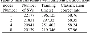
In this example, C-SVC model is adopted. The parameter of the SVM model is set as follows. Constant C is set 1, radial basis function is taken as kernel function, and gamma is set as 0.01. Firstly, the example is analyzed with only 1 computation node, i.e. classical SVM method is used to train the SVM model. The trained model is used to predict the testing samples. The training time and classification correct rate are listed in Table 2. Secondly, the example is analyzed with the parallel SVM based on map/reduce. For comparison, the sample is partitioned into 2, 3, 4, 5 sub-samples respectively. When the sample is partitioned into 2 sub-samples, 2 computing nodes are used. The training time and classification rate corresponding to each partition form are listed in table 3.

Table 3 analysis results with different partition nodes nodes

Number

Number of SVs

Training time(s)

Classification correct rate

1 22177 396.125 58.76

2 21831 297.32 58.35

4 20941 251.402 58.24

8 20139 219.346 57.96

5.2.4 Feature selection with correlation coefficient

In the example, there are 54 attribute variables. Most variables provide minor contribution in the classification, especially the Soil_Type variables. For improve the training speed and reduce the noise effect of attribute variables, correlation coefficient Eq. (9) is used to select attribute variables. After calculating the correlation coefficient, the

1 2 3 4 5 6 7 8

50 100 150 200 250 300 350 400 450 500

nodes number

tr

ai

ni

ng t

im

e(

s

)

all variable feature selection

1 2 3 4 5 6 7 8

82.5 83 83.5 84 84.5 85

nodes number

c

or

rec

t per

c

ent

(%

)

pruning value is set 0.1. At last, 18 attribute variables are selected. The training result is listed in table 4.

Table 4 analysis result of SVM based on feature selection Number of nodes Number of SVs Training time(s) Classification correct rate

1 14624 82.022 57.46

2 14198 58.899 57.99

4 13298 55.154 58.57

8 12207 45.029 58.65

5.2.5 Result analysis

This example is a multiclass classification problem. How to improve classification correct rate of multi-class is still a big problem. From Fig.5 we can find that the training time can be reduced greatly when the sample is partitioned 2 parts. But with the increase of partition number, the training time reduction will become slow. In this example, the ratio

α ≈0.4 and β ≈1.2. It is similar to the analysis problem of example 1. With the introduction of feature selection, the computation can be reduced greatly. From the analysis correct rate we can find that correct rate will not decrease too much.

Fig. 5 training time based on different partition nodes

Fig. 6 Correct rate based on different partition

5.3

Heart disease classification

5.3.1 Data source

There are 270 clinic reports. Each report includes 13 factor variables. Clinic is divided into 2 classes. For testing the efficiency of the proposed cascade SVM, we replicate the data 500 times, 1000 times, and 2000 times separately. The generated data sets has 135000, 270000, 540000 samples separately. The initial data set is used to test the SVM model. The training time and correct rates based on different partition styles are listed in table 5, table 6 and table 7 respectively.

Table 5 analysis result with data replicated 500 times

Number of nodes Number of SVs Training time(s) Classification correct rate

1 7585 313.755 99.629

2 7712 148.184 99.259

4 7690 87.523 98.518

8 7487 76.773 98.148

Table 6 analysis result with data replicated 1000 times

Number of nodes Number of SVs Training time(s) Classification correct rate

1 8972 539.28 100

2 9055 234.49 99.63

4 8739 123.887 98.15

8 8688 86.503 97.41

Table 7 analysis result with data replicated 2000 times

Number of nodes Number of SVs Training time(s) Classification correct rate

1 N/A N/A N/A

2 9901 578.507 100

4 9650 266.587 99.63

8 9202 158.531 99.63

The analysis result is shown as in figure 7, figure 8 and figure 9.

Figure 7 training time based on different partition nodes

Figure 8 Correct rate based on different partition

Fig. 9 training time based on different parallelism corresponding to different sample size

5.3.2 Result analysis

From the above analysis results we can find that the bigger the sample size the more obvious of the speed up.

1 2 3 4 5 6 7 8

0 50 100 150 200 250 300 350 400 nodes number tr ai ni ng t im e( s ) all variable feature selection

1 2 3 4 5 6 7 8

57.4 57.6 57.8 58 58.2 58.4 58.6 58.8 nodes number c or rec t per c ent (% ) all variable feature selection

1 2 3 4 5 6 7 8

0 100 200 300 400 500 600 nodes number tr ai ni ng t im e( s )

data copy 2000 times data copy 1000 times data copy 2000 times

1 2 3 4 5 6 7 8

97 97.5 98 98.5 99 99.5 100 nodes number c o rre c t ra te (% )

data copy 2000 times data copy 1000 times data copy 2000 times

1 2 3 4

From figure 7, we can find that when the sample size is very big, i.e. 540000 samples, it can’t be processed with one single computation node. It is out of the memory. It is necessary to process big size problem with parallel style. The training time will decrease slowly when the parathion number is bigger than 8. It is because of two reasons. The first reason is that he ratio between optimum computation time and data transform overhead is less. The other reason is that the sample size of the last level can’t be less than the number of support vectors. The computation cost will account a big proportion. So the computation will decrease very slowly. From fig. 9 we can find the computation time based on different partition style is approximate linear relationship to sample size.

6

Conclusions

Data-intensive data mining is still a big problems faced by computer scientist. SVM is taken as a most efficient classification and regression model. The computation cost of SVM is square proportion to the number of training data. Classical SVM model is difficult to analyze large scale practical problems. Parallel SVM can improve the computation speed greatly. In this paper, parallel SVM model based on iterative MapReduce is proposed. It is realized with Twister software. Through example analysis it shows that the proposed cascade SVM based on Twister can reduce the computation time greatly. But it doesn't mean that it is better to partition sample data into many parts. The computation time will not decrease through the analysis of the computation time. The partition number can be estimated according to the concrete problems. For increase the computation speed, the cascade SVM can be combined with other feature selection and feature extraction methods. In total, the analysis results show that the parallel SVM based on iterative MapReduce is efficient in data intensive problems.

Acknowledgements

This work is partially supported by Provincial Outstanding Research Award Fund for young scientist (No. BS2009DX016) and Provincial Fund for Nature project (No. ZR2009FM038).

References

[1] J R Swedlow, G Zanetti, C Best. “Channeling the data deluge”. Nature Methods, 2011, 8: 463-465.

[2] G C Fox, X H Qiu et al. “Case Studies in Data Intensive Computing: Large Scale DNA Sequence Analysis.” The Million Sequence Challenge and Biomedical Computing Technical Report, 2009

[3] X H Qiu, J Ekanayake, G C Fox et al. “Computational Methods for Large Scale DNA Data Analysis.” Microsoft eScience workshop, 2009

[4] J A Blake, C J Bult. Beyond the data deluge: “Data integration and bio-ontologies.” Journal of Biomedical Informatics, 2006, 39(3), 314-320.

[5] J Qiu. “Scalable Programming and Algorithms for Data Intensive Life Science.” Applications Data-Intensive Sciences Workshop, 2010

[6] R Guha, K Gilbert, G C Fox, et al. “Advances in Cheminformatics Methodologies and Infrastructure to Support the Data Mining of Large, Heterogeneous Chemical Datasets.” Current Computer-Aided Drug Design, 2010, 6: 50-67.

[7] C C Chang, B He, Z Zhang. “Mining semantics for large scale integration on the web: evidences, insights, and challenges.” SIGKDD Explorations, 2004: 6(2):67-76.

[8] G C Fox, S H Bae, et al. “Parallel Data Mining from Multicore to Cloudy Grids.” High Performance Computing and Grids workshop, 2008

[9] B J Zhang, Y Ruan et al. “Applying Twister to Scientific Applications.” Proceedings of CloudCom, 2010

[10]J Ekanayake, H Li, et al. “Twister: A Runtime for iterative MapReduce.” The First International Workshop on MapReduce and its Applications of ACM HPDC, 2010

[11]C. Cortes, V. Vapnik. “Support Vector Networks.” Machine Learning,1995, 20: 273-297

[12]C C Chang, C J Lin. “LIBSVM: a library for support vector machines.” ACM Transactions on Intelligent Systems and Technology, 2011, 27(2): 1-27.

[13]B Boser, I Guyon, V Vapnik. “A training algorithm for optimal margin classifiers.” The 5th Annual Workshop on Computational Learning Theory, 1992.

[14]R E Fan, P H Chen, C J Lin. “Working set selection using second order information for training SVM.” Journal of Machine Learning Research, 2005, 6: 1889-1918.

[15]H P Graf, E Cosatto, et al. “Parallel support vector machines: the Cascade SVM.” Advances in Neural Information Processing Systems, MIT Press, 2005. [16]A Tveit, H Engum. “Parallelization of the Incremental

Proximal Support Vector Machine Classifier using a Heap-based Tree Topology.” Tech. Report, IDI, NTNU, Trondheim, 2003.