This is a repository copy of Accuracy of Eulerian–Eulerian, two-fluid CFD boiling models of subcooled boiling flows.
White Rose Research Online URL for this paper: http://eprints.whiterose.ac.uk/102976/
Version: Accepted Version
Article:
Colombo, M and Fairweather, M (2016) Accuracy of Eulerian–Eulerian, two-fluid CFD boiling models of subcooled boiling flows. International Journal of Heat and Mass Transfer, 103. pp. 28-44. ISSN 0017-9310
https://doi.org/10.1016/j.ijheatmasstransfer.2016.06.098
© 2016, Elsevier. Licensed under the Creative Commons Attribution-NonCommercial-NoDerivatives 4.0 International http://creativecommons.org/licenses/by-nc-nd/4.0/
[email protected] https://eprints.whiterose.ac.uk/
Reuse
Unless indicated otherwise, fulltext items are protected by copyright with all rights reserved. The copyright exception in section 29 of the Copyright, Designs and Patents Act 1988 allows the making of a single copy solely for the purpose of non-commercial research or private study within the limits of fair dealing. The publisher or other rights-holder may allow further reproduction and re-use of this version - refer to the White Rose Research Online record for this item. Where records identify the publisher as the copyright holder, users can verify any specific terms of use on the publisher’s website.
Takedown
If you consider content in White Rose Research Online to be in breach of UK law, please notify us by
Accuracy of Eulerian – Eulerian, two-fluid CFD boiling
1
models of subcooled boiling flows
2 3
M. Colombo* and M. Fairweather 4
School of Chemical and Process Engineering, University of Leeds, Leeds LS2 9JT, United 5
Kingdom 6
E-mail addresses: [email protected], [email protected] 7
8
*Corresponding Author. Tel: +44 (0) 113 343 2351 9
10
ABSTRACT
11
Boiling flows are frequently found in industry and engineering due to the large amount of 12
heat that can be transferred within such flows with minimum temperature differences. In the 13
nuclear industry, boiling affects in different ways the operation of almost all water-cooled 14
nuclear reactors. Recently, the use of Computational fluid dynamic (CFD) approaches to 15
predict boiling flows is increasing and, in the nuclear area, CFD is being developed to solve 16
thermal hydraulic safety issues such as establishing the critical heat flux, which is perhaps the 17
major threat to the integrity of nuclear fuel rods. In this paper, the accuracy of an Eulerian – 18
Eulerian, two-fluid CFD model is evaluated over a large database of subcooled boiling flows, 19
avoiding the rather popular case-by-case tuning of descriptive models to a limited number of 20
experiments. The model includes a Reynolds stress turbulence model, the method of 21
moments-based S population balance approach and a boiling model derived using the heat
22
flux partitioning approach. The database covers a large range of conditions in subcooled 23
boiling flows of water and refrigerants in vertical pipes and annular channels. Overall, a 24
satisfactory predictive accuracy is achieved for some quantities of interest, such as the void 25
fraction and the turbulence and liquid temperature fields, but results are less satisfactory in 26
other areas, more specifically for the average bubble diameter and the mean velocity profiles 27
close to the wall in annular channels. Agreement may be improved with advances in the 28
treatment of large bubbles and bubble break-up and coalescence, as well as in improved 29
modelling of the boiling region close to the wall, and more specifically the bubble departure 30
diameter, the wall treatment and the contribution of bubbles to turbulence. 31
32
KEYWORDS: Subcooled boiling; computational fluid dynamics; two-fluid model; heat-flux 33
partitioning; boiling model. 34
1
Introduction
39 40
In industry, boiling flows are often encountered because of the efficiency of heat transfer 41
mechanisms under such conditions, which allow the transfer of significant amounts of heat 42
with a limited amount of wall superheat, to the benefit of many engineering processes. In the 43
nuclear industry, different types of boiling regimes are found in all water-cooled reactors, 44
both in normal operation and during design-basis and beyond design-basis postulated 45
accident transients. Boiling water reactors operate in the saturated boiling regime, and some 46
degree of subcooled boiling is always experienced in pressurized water reactors during 47
normal operation. Buoyancy-driven natural circulation loops and safety systems are also 48
sometimes designed to operate within the boiling regime and, during loss of coolant accidents 49
for example, boiling may occur due to the decrease in pressure and the reduced coolant 50
inventory. For a reactor experiencing boiling conditions, the maximum amount of heat 51
transferrable from the nuclear fuel to the coolant is referred to as the critical heat flux (CHF) 52
and, when this is reached, the heat transfer deteriorates rapidly [1,2]. Recently, a significant 53
portion of nuclear reactor thermal hydraulic analyses make use of multiphase computational 54
fluid dynamic (CFD) models, and in particular of the Eulerian-Eulerian, averaged two-fluid 55
formulation that is invariably used when addressing industrial-scale engineering problems. 56
With respect to the simplistic models more commonly used in the nuclear industry, CFD may 57
ultimately be able to describe phenomena in much greater detail, leading to the solution of 58
selected nuclear reactor thermal hydraulic safety issues [3], including the prediction of CHF 59
which, despite being perhaps the main threat to the integrity of nuclear fuel rods and despite 60
long-term research efforts, has still resisted accurate modelling and understanding [4]. 61
With the aim of predicting the boiling process, different wall boiling models have been 62
incorporated in modern CFD codes. For two-fluid averaged models, these approaches are in 63
the large majority based on the Rensselaer Polytechnic Institute (RPI) boiling model from 64
Kurul and Podowski [5], where the heat flux from the wall is partitioned between the 65
mechanisms responsible for the heat transfer process, these being single-phase convection, 66
quenching and evaporation. In recent years, many authors have used more or less refined 67
versions of the RPI boiling model to predict boiling flows [6-12]. After departure from the 68
heated wall, the bubbles join the bulk of the flow and the size distribution of these bubbles, 69
polydispersed in general, governs interphase exchanges of mass, momentum and energy. 70
Therefore, in models of these flows, knowledge of the average diameter of the bubbles is 71
average bubble diameter distribution. Initially, bubble size was derived from experimental 73
data or empirical correlations of subcooling in the liquid phase [5,13-16]. More recently, 74
bubble size distribution has been predicted by coupling different population balance 75
approaches to the two-fluid and the wall boiling models. Yao and Morel [6] derived source 76
terms for bubble coalescence, bubble break-up and phase change to be used in the volumetric 77
interfacial area transport equation. Yeoh and Tu [7] added wall nucleation and condensation 78
in the bulk flow to the multiple size group (MUSIG) model [17], which divides the bubble 79
diameter spectrum into a finite number of ranges to accommodate non-uniform bubble size 80
distributions. All these authors reported significant improvements over predictions based on 81
empirical correlations of subcooling of the liquid phase. More recently, Krepper et al. [10] 82
applied the inhomogeneous version of the MUSIG model, where each bubble size range is 83
allowed to have its own velocity, to the simulation of a subcooled boiling flow in a vertical 84
pipe. Morel and Lavieville [18] extended to boiling flows a method based on conservation of 85
the density S of the moments of the bubble size distribution, which was assumed to obey to a 86
log-normal probability distribution. In their model, bubble break-up was not accounted for. 87
Bubble break-up was considered in the context of the S model, initially proposed by Lo and 88
Rao [19] and Lo and Zhang [20], by Yun et al. [9], and more recently by Thakrar et al. [12], 89
to simulate boiling flows in a vertical pipe and in a vertical rectangular channel, respectively. 90
The boiling model calculates the amount of vapour generated at the wall and the 91
corresponding mass source is added to the near-wall computational cell. Here, in the large 92
majority of CFD codes, the boundary condition on the flow field is imposed using wall 93
functions. Wall functions for use in boiling flows have been developed by different authors 94
by including, in the single-phase law of the wall, an additional roughness due to the bubbles 95
attached at the wall [8,10,14]. 96
Most of the boiling models have been tested against experimental measurements made in 97
subcooled boiling flows. The majority of these experiments were performed in circular cross-98
section geometries, with water at low pressure [13] or refrigerant at moderate pressure [21-99
23], because they scale to typical operating conditions found in water-cooled nuclear reactors. 100
At high pressure, the availability of data is more limited and the axial averaged void profiles 101
measured by Bartlomej and Chanturiya [24] and Bartolomej et al. [25] in upward pipe water 102
flows are perhaps the most extensively investigated case to date, in addition to the DEBORA 103
experiment [22], which, instead, focused on the boiling of refrigerant R12 at moderate 104
pressures. At high pressure, the measurements of Pierre and Bankoff [26] in a rectangular 105
In the majority of works to date, the boiling model is tested against a single experiment and, 107
most frequently, a good predictive accuracy is demonstrated, but generally after calibration or 108
tuning of some of the model parameters to the experiment under study [7,9,10,15]. Even if 109
built in a mechanistic fashion, all the RPI-based models available at present are actually 110
forced to rely on some empirical or semi-empirical closure relation, in particular for the 111
evaporative heat transfer contribution, which requires knowledge of the active nucleation site 112
density and the bubble departure diameter and frequency. The numerous empirical 113
correlations available for this purpose were recently reviewed by Cheung et al. [27] and 114
Thakrar et al. [28]. In general, poor predictive accuracy of these models has been found for 115
subcooled boiling data over a wide range of mass and wall heat fluxes, and inlet subcooling, 116
and no combination of correlations that provide a satisfactory overall accuracy has been 117
identified. In the context of CFD, the most used correlations have been those of Lemmert and 118
Chawla [29] and Hibiki and Ishii [30] for the active nucleation site density, of Tolubinsky 119
and Kostanchuk [31] and Kocamustafaogullari [32] for the bubble departure diameter, and of 120
Cole [33] for the bubble departure frequency [7,8,10,12,16]. However, attempts to assess the 121
accuracy of these correlations for the conditions simulated are rather scarce, and no definitive 122
information on the range of parameters over which any correlation is expected to provide a 123
satisfactory accuracy, or simply outperform other correlations, is available. In view of these 124
deficiencies, some authors have recently started to use more mechanistic formulations based 125
on a balance of the forces acting on the growing bubble to calculate the bubble departure 126
diameter [9,34]. 127
In this paper, a large database of subcooled boiling flows in vertical channels examined 128
experimentally over a wide range of operating conditions is assembled and predicted using a 129
model solved using the STAR-CCM+ code. It has recently been noted [35,36] how it is 130
necessary, to make progress in this field, to have models that are validated against numerous 131
experiments, rather than on a case-by-case basis which only provides good agreement with a 132
single experiment. This is particularly the case in the qualification of two-phase flow CFD 133
codes for nuclear safety applications. In view of this, changes to any model should only be 134
made if they are based on sound physical considerations, and following improvements to the 135
overall performance of the model [35,36]. In this work, a priori selected closure models are 136
applied to the whole database and the global accuracy of the model is evaluated (although 137
some changes were necessary and will be explained throughout the text). The two-phase flow 138
is described using an Eulerian-Eulerian two-fluid model, with boiling at the wall accounted 139
bubble size distribution, is used to predict the bubble diameter distribution, which governs the 141
interfacial area density and therefore the interphase transfer processes. A multiphase 142
Reynolds stress turbulence model is used, which, to the authors’ knowledge, represents a 143
level of closure in the context of boiling flows which has only been employed by Mimouni et 144
al. [37,38] to predict the two-phase flow in a fuel bundle subjected to the influence of a 145
mixing vane. Therefore, the impact of the use of a second-moment turbulence closure in 146
subcooled boiling simulations is further investigated. In view of the large database adopted, 147
the overall ability of multiphase CFD approaches to predict general boiling flows is 148
evaluated, this being a necessary step if models of this kind are to be confidently applied to 149
the prediction of the CHF. Areas that need further improvement are also identified and their 150
impact on the global accuracy of the model is tested. Amongst others, the multiphase 151
turbulence model and models for bubble coalescence and break-up, which are often one of 152
the weakest aspects in the simulation of bubbly flows [36], are identified. 153
154
2
Model description
155 156
In a two-fluid Eulerian-Eulerian model, each phase is described by a set of averaged 157
conservation equations, and the continuity, momentum and energy equations are solved for 158
each phase. These, being discussed for adiabatic two-phase boiling flows in many previous 159
publications [7,39,40] to which the interested reader may refer to, are not presented here. As 160
a consequence of the averaging procedure, details of the interphase structure are lost and 161
closure models are required for the mass, momentum and energy transfers at the interphase. 162
These, and in particular the interphase momentum exchanges, have received much attention 163
in recent years [41,42]. In this work, the drag model of Tomiyama et al. [43] is used, where 164
the drag coefficient CD is calculated from the bubble Reynolds and Eötvös numbers, Re and
165
Eo: 166
167
(1)
168
A lift force, perpendicular to the direction of motion, is experienced by bubbles moving in a 169
shear flow [44] and this influences the radial void distribution in pipe and channel flows. 170
Spherical bubbles are pushed towards the pipe wall whereas larger bubbles, which are more 171
often oblate and ellipsoidal because of the inertia of the surrounding liquid, experience, after 172
towards the centre of the pipe [45]. In the literature, different correlations are available for 174
the lift coefficient that also predict the change of sign with bubble diameter [45]. The wall 175
force, in contrast, tends to keep bubbles away from a solid wall, and was modelled first by 176
Antal et al. [46]. Lift and wall forces in adiabatic bubbly flows are fairly well established, 177
although some uncertainties in their effective contributions, or in the actual accuracy of the 178
available models, still exist [47,48]. Proof of the latter is found in the numerous different 179
models that authors have used, even in the recent past. The use of lift and wall forces in 180
boiling flows is much more uncertain and more general studies on the behaviour of bubbles 181
near the heated wall are necessary. In view of these uncertainties, lift and wall forces were 182
generally neglected. The turbulent dispersion force is modelled following Burns et al. [49], 183
with a turbulent dispersion coefficient CTD = 2.5 and a turbulent Prandtl number = 1.0
184
[49]: 185
186
(2)
187
2.1 Multiphase turbulence modelling
188 189
Turbulence is solved in the continuous phase only, with a Reynolds stress model (RSM) 190
based on a multiphase formulation of the single-phase model due to Speziale, Sarkar and 191
Gatsky (SSG) [50, 51]: 192
193
(3)
194
Here, Pij is the turbulence production, the diffusion Dij is modelled accordingly to Daly and
195
Harlow [52] and the isotropic hypothesis is used for the turbulence energy dissipation rate ij.
196
The pressure-strain correlation ij, accounting for pressure fluctuations that redistribute the
197
turbulence kinetic energy amongst the normal Reynolds stresses, is quadratically non-linear 198
in the anisotropy tensor [50]. In the dispersed phase, turbulence was not resolved, but was 199
instead directly related to the turbulence of the continuous phase by means of a response 200
coefficient Ct, assumed equal to unity [53,54] following experimental evidence that suggests
201
With respect to a single-phase flow, the generation of turbulence by bubbles can modify 203
significantly the turbulence in the continuous phase [56-58]. To account for this contribution, 204
bubble-induced source terms were included in the turbulence model assuming that all the 205
energy lost by the bubbles to drag is converted into turbulence kinetic energy inside the 206
bubble wakes [54, 59, 60]: 207
208
(4)
209
The corresponding turbulence energy dissipation rate source is equal to the turbulence 210
kinetic energy source divided by the timescale of the bubble-induced turbulence, calculated 211
from the velocity scale of the turbulence and the length scale of the bubbles [60]: 212
213
(5)
214
The mixed timescale, used in combination with the coefficient KBI = 0.25, has been found to
215
provide accurate predictions over a wide range of bubbly pipe flows [61]. The need for a 216
bubble-induced turbulence contribution in bubbly flows has been demonstrated in many 217
previous studies [48,54,60]. In contrast, less established is the use of these bubble-induced 218
turbulence models in boiling flows and, therefore, this specific issue is further discussed in a 219
specific section within the Results and discussion. 220
221
2.2 The S model
222 223
Bubbles, after departure from the heated wall, experience evaporation and condensation in 224
the bulk of the flow, and break-up and coalescence events that alter the bubble diameter 225
distribution and affect the interphase mass, momentum and energy exchanges. The bubble 226
diameter distribution is predicted with the S model [19,20], where it is assumed to obey to a 227
pre-defined log-normal probability distribution P(dB). From this, the density of the moments
228
of the bubble size distribution M may be derived: 229
230
(6)
The zeroth order moment is equal to the bubble number density n, whereas S
2 and S3 are
232
closely related to the interfacial area concentration and the void fraction: 233
234
(7)
235
Average diameters of different kinds of bubble are obtained by combining the moment 236
densities, including, from S2 and S3, the Sauter-mean diameter (SMD), which is compared
237
against experiments later: 238
239
(8)
240
Additionally, the variance of the distribution is calculated from: 241
242
ln ln (9)
243
The two average diameters, d32 and d30, are equal only for a monodispersed distribution.
244
Since the void fraction is known from the two-fluid model, the solution of only two 245
additional equations for S0 and S2 is sufficient to characterize the bubble size distribution. For
246
each moment, a transport equation of the following type needs to be solved: 247
248
(10)
249
The source terms account for the contributions of bubble break-up and coalescence, with the 250
last being the source due to boiling at the wall and condensation/evaporation in the bulk of 251
the flow: 252
253
(11)
In this work, interactions induced by turbulence were assumed to be dominant and the only 255
mechanism inducing break-up and coalescence events [6,20]. The source term for bubble 256
break-up is expressed as: 257
258
(12)
259
where Kbr is the break-up rate, the reciprocal of the break-up time br, and Sbr is the change
260
in S due to a single break-up event, which, from conservation of volume, is: 261
262
(13)
263
The number of daughter bubbles Nf was assumed equal to 2 [6,20,62]. The break-up
264
timescale follows from the frequency of the second oscillation mode of a droplet [20]: 265
266
(14)
267
with kbr = 0.2. Bubbles break when the Weber number is higher than a critical value Wecrit,
268
equal to 1.24 [6,48]: 269
270
(15)
271
C , equal to 4.6, is a correction factor that accounts for nearby bubbles that disrupt the 272
influence of the surrounding inertial forces. The general source term for bubble coalescence 273
is: 274
275
(16)
276
Here, is the coalescence rate between two bubbles with diameters d and d’, and 277
computational cost, it is assumed, in the coalescence source term, that the bubble diameter 279
has a uniform distribution with an equivalent mean diameter, taken equal to the SMD. 280
Therefore, the change in S due to a single coalescence event becomes: 281
282
(17)
283
From Yao and Morel [6], the number of coalescence events per unit volume and unit time is 284
expressed as: 285
286
(18)
287
The first part of Eq. (18) represents the collision rate between the bubbles, whilst the 288
exponential function describes the probability of coalescence following a collision event. 289
The function g( ) accounts for the effect of the packing of the bubbles when the void fraction 290
is higher than a certain value. From [6], C1 = 2.86, C2 = 1.922, C3 = 1.017 and Wecrit = 1.24.
291
292
2.3 Boiling model
293 294
When boiling occurs at a heated wall, different heat transfer mechanisms take place and 295
these need to be modelled. In regions of the wall where no bubbles are growing, the heat is 296
transferred to the liquid by single-phase convection. Otherwise, the heat is removed by the 297
evaporation process and supports the growth of bubbles at the nucleation sites. Bubbles grow 298
attached to the wall until, when certain conditions are reached, detachment occurs. 299
Detachment of bubbles promotes additional mixing in the fluid phase and the recirculation of 300
subcooled liquid which is brought into contact with the wall to fill the volume which was 301
previously occupied by the detaching bubble. This mechanism accounts for a portion of the 302
heat transferred from the wall, and is known as quenching. Finally, when a significant 303
amount of vapour is present at the wall, liquid access to the wall may be restricted and a 304
portion of the heat is transferred by convection to the vapour phase. Therefore, and following 305
the RPI model of Kurul and Podowski [5], the total heat transferred from the wall is 306
partitioned between these heat transfer mechanisms: 307
308
309
Kdry is the fraction of the wall in contact with the vapour which becomes larger than zero
310
when the void fraction is higher than a critical value, assumed equal to 0.9 [51]. The single-311
phase convective volumetric heat flux to the liquid phase is obtained from: 312
313
(20)
314
Ab is the fraction of the wall influenced by the evaporation process and T+a dimensionless
315
temperature, which is calculated using the wall function approach [51]. In the same way, the 316
convective volumetric heat flux to the vapour phase is known from: 317
318
(21)
319
The quenching volumetric heat flux, which accounts for the additional heat transfer to the 320
cooler liquid that replaces a bubble detaching from the wall, is given by: 321
322
(22)
323
The quenching heat transfer coefficient is modelled accordingly to Del Valle and Kenning 324
[63]: 325
326
(23)
327
In the previous equation, tw is the waiting time between the bubble departure and the
328
nucleation of the next bubble: 329
330
(24)
331
In Eq. (22), and to avoid any dependency on the computational grid employed, the liquid 332
temperature is evaluated at a constant y+ of 250.
The evaporative volumetric heat flux is known from the number of bubbles that grow 334
attached to the heated wall at the active nucleation sites. These bubbles grow until the forces 335
that promote detachment overcome those that keep the bubble attached to the wall. Therefore, 336
the evaporative heat flux is known from the number of active nucleation sites, the diameter of 337
the bubbles at departure and the frequency of the bubble departure from the wall: 338
339
(25)
340
In Eq. (25), closure relations are required for the nucleation site density, the bubble departure 341
diameter and the bubble departure frequency. Most often, these have been obtained from 342
empirical correlations. Only recently have more mechanistic formulations been introduced to 343
calculate the bubble departure diameter [9,34]. In this work, two correlations for both the 344
nucleation site density and for the bubble departure diameter are considered. Lemmert and 345
Chawla [29] proposed correlating the nucleation site number density to the wall superheat: 346
347
(26)
348
with n0 = 12366.45 m-2K-1 and p = 1.805. More recently, it has become evident that, to have a
349
model with a wide applicability, correlation to other parameters has to be taken into account, 350
including properties of the heated surface such as the contact angle [30]. The more recent 351
model from Hibiki and Ishii [30] is given by: 352
353
(27)
354
where n0 = 4.72 × 10⁵ m-2, ’ = 0.722 rad and ’ = 2.50 × 10⁻⁶ m. is the contact angle, f’a
355
function of + = log (∆ /
v) and Rc is equal to:
356
357
(28)
358
Tolubinsky and Kostanchuk [31] correlated the bubble departure diameter to the liquid 359
361
(29)
362
Here, d0 = 0.0006 m and ∆T0 = 45 K. Kocamustafaogullari [32] developed a model for the
363
bubble departure diameter based on a balance between gravity and surface tension forces. 364
The model, with the addition of the dependency on a density ratio, was developed to account 365
for the effect of the system pressure: 366
367
(30)
368
where dl = 1.5126 × 10⁻³ m rad-1 and = 0.722 rad for water systems. The bubble departure
369
frequency is calculated from Cole [33]: 370
371
(31)
372
The fraction of the wall affected by the evaporation process is known from [5]: 373
374
(32)
375
Finally, in the bulk of the fluid, the liquid side heat transfer coefficient at the interphase is 376
calculated using the Ranz and Marshall [64] correlation: 377
378
(33)
379
The overall model, implemented in the STAR-CCM+ CFD code [51], is solved in a two-380
dimensional axisymmetric geometry. At the inlet, fully-developed single-phase liquid 381
velocity, turbulence and temperature are imposed, together with an imposed pressure at the 382
outlet and the no-slip condition, and an imposed heat flux, at the wall. Strict convergence of 383
residuals was ensured, together with a mass balance error always lower than 0.01 % for both 384
with an equidistant structured mesh with the first grid point placed at a minimum wall 386
distance of y+ = 30, which is the lower limit for the use of wall functions.
387
388
3
Experimental data
389 390
Confidence in the predictions of CFD codes relies on extensive validation of their results 391
against relevant experimental data. In this regard, it is important that models provide accurate 392
predictions over many experiments, with parameter variations as wide as possible. Therefore, 393
a database was built from 20 experiments from 5 different sources: Bartlomej and Chanturiya 394
[24], Bartolomej et al. [25], Roy et al. [21], the DEBORA experiment [22] and Lee et al. 395
[13]. The database, which is summarized in Table 1, includes measurements in vertical pipes 396
and annular channels of subcooled boiling flows of water, Freon-12 and refrigerant R-113, 397
and covers the ranges 0.101 – 6.89 MPa for the pressure, 477 – 2981 kg m-2s-1 for the mass 398
flux, 58.2 – 1200 kW m-2 for the heat flux and 11.5 – 63 °C for the inlet subcooling.
399
The DEBORA [22] flow loop consisted of a 19.2 mm inner diameter vertical pipe, heated for 400
a length of 3.5 m and operated with Freon-12 (R-12). Given the inherent difficulties of 401
measuring the flow boiling of water at high pressure, and temperature, Freon-12 guaranteed 402
more favourable experimental conditions, while maintaining values of dimensionless groups 403
such as the Reynolds and the Weber number, and the density ratio, consistent with typical 404
operating conditions of pressurized water reactors. Measurements were taken in the ranges 405
1.46 – 3.01 MPa for the pressure, 1000 – 3000 kg m-2s-1 for the mass flux and 58 – 135 kW
406
m-2 for the heat flux, and a significant range of liquid subcooling. Void fraction and vapour
407
velocity profiles at the end of the test section were measured with an optical probe technique, 408
from which radial profiles of the interfacial area concentration and the SMD were 409
determined. Thermocouples were used to measure the liquid temperature radial profile and 410
the wall temperature at selected axial locations. 411
Batolomej and Chanturiya [24], and Bartolomej et al. [25], investigated the subcooled boiling 412
of water in vertical pipes of inlet diameter D = 0.0154 m and 0.012 m, and length L = 2 m 413
and 1.4 m, respectively. Average void fractions were measured at different axial locations at 414
pressures up to 15 MPa, mass fluxes up to 2000 kg m-2s-1 and heat fluxes up to 2.2 MW m-2. 415
For this study, five cases were selected from these experiments at pressures up to 6.89 MPa, 416
mass fluxes up to 1500 kg m-2s-2 and heat fluxes up to 1.2 MW m-2 (Table 1). 417
Roy et al. [21] tested the subcooled boiling of refrigerant R-113 in a vertical annulus of 3.66 418
velocimetry system allowed measurement of the velocity field and the turbulent fluctuations, 420
with an optical probe used to obtain the void fraction and the bubble diameter. The liquid and 421
vapour temperatures were measured with micro-thermocouples. Measurements were taken at 422
0.269 MPa and in the ranges 565 – 785 kg m-2s-1 for the mass flux, 79.4 – 125.9 kW m-2 for
423
the heat flux and 42.7 – 50.2 °C for the inlet temperature. In a slightly different annular 424
channel, 2.376 m in length, 0.019 m in inlet diameter and 0.0375 m in outlet diameter, Lee et 425
al. [13] investigated the subcooled flow boiling of water at nearly atmospheric pressure, and 426
474 – 1061 kg m-2s-1 for the mass flux, 115 – 300 kW m-2 for the heat flux and 11.5 – 21.3 °C
427
for the inlet subcooling. Liquid velocity radial profiles were measured with a Pitot tube, and 428
vapour velocity and void fraction radial profiles with a two-conductivity probe method. 429
None of the previous experiments provides a complete characterization of the flow, which is 430
a shortcoming of most of the experimental data available to date. Limited measurements of 431
the bubble diameter are available from Roy et al. [21] and, therefore, the DEBORA 432
experiment is the only one that provides radial profiles of the average bubble diameter. 433
However, in the DEBORA experiment, liquid velocity profiles and liquid turbulence profiles 434
were not measured. Turbulence profiles, in particular, are only available from Roy et al. [21]. 435
Temperatures were measured in the DEBORA and the Roy et al. [21] experiments, but not 436
by Lee et al. [13], which also did not provide any information on liquid turbulence and 437
bubble diameter. Finally, in Bartolomej and Chanturiya [24] and Bartolomej et al. [25], and 438
since these experiments were undertaken at higher pressures and some decades ago, only the 439
average void fraction at different axial locations was measured. Even so, these experiments 440
are one of the few to give measurements at high pressure. The use of a large database 441
therefore overcame the limitation of each individual dataset, allowing validation of the model 442
for all physical quantities of interest. It is important to note, however, the necessity for more 443
detailed and comprehensive experimental data sets in order to improve our ability to predict 444
these kinds of flows, since, as will be seen in the following section, the parameters of interest 445
interact with each other in a rather complex and non-linear way. 446
Table 1. Summary of the experimental conditions included in the validation database. 455
Data Source p [MPa] pr [-] G [kg m-2s-1] q” [kW m-2] Tin [°C] Fluid Geometry
deb1 Garnier et al. [22] 2.62 0.63 1996 73.9 68.5 R12 P
deb2 Garnier et al. [22] 2.62 0.63 1985 73.9 70.5 R12 P
deb3 Garnier et al. [22] 1.46 0.35 2023 76.3 39.7 R12 P
deb4 Garnier et al. [22] 1.46 0.35 2028 76.2 34.9 R12 P
deb5 Garnier et al. [22] 2.62 0.63 2981 109.4 69.2 R12 P
deb6 Garnier et al. [22] 3.01 0.73 1007 58.2 64.6 R12 P
roy1 Roy et al. [21] 0.269 0.08 565 79.4 42.7 R113 A
roy2 Roy et al. [21] 0.269 0.08 785 95.0 50.2 R113 A
roy3 Roy et al. [21] 0.269 0.08 785 125.9 50.2 R113 A
lee1 Lee et al. [13] atm 0.005 478 152.8 80.8 W A
lee2 Lee et al. [13] atm 0.005 477 114.8 88.5 W A
lee3 Lee et al. [13] atm 0.005 718 232.6 78.8 W A
lee4 Lee et al. [13] atm 0.005 714 197.2 86.2 W A
lee5 Lee et al. [13] atm 0.005 1061 300.0 81.9 W A
lee6 Lee et al. [13] atm 0.005 1047 251.2 86.6 W A
bar1 Chanturiya [24] Bartolomej and 1.5 0.07 900 380 138.3 W P
bar2 Chanturiya [24] Bartolomej and 4.5 0.20 900 570 197.4 W P
bar3 Bartolomej et al. [25] 6.89 0.31 1500 1200 221.9 W P
bar4 Bartolomej et al. [25] 6.89 0.31 1500 800 245.9 W P
bar5 Bartolomej et al. [25] 6.89 0.31 1000 800 229.9 W P
atm = atmospheric; W = water; P = pipe; A = annular channel. 456
457
4
Results and discussion
458 459
4.1 Coalescence source
460 461
Before simulating the whole database, some model parameters had to be selected, starting 462
with the coalescence source, calculated from Yao and Morel [6]. In a previous work, a critical 463
Weber number Wecrit = 0.10 in the coalescence efficiency allowed good agreement to be
464
obtained for different air-water bubbly flows in vertical pipes [65]. This agreement was 465
achieved in combination with the assumption of negligible bubble break-up, which is 466
expected to be even lower in boiling flows due to the lower expected bubble diameter. In 467
bubbly flow experiments, therefore, bubbles are usually injected with a diameter of the order 468
of a few millimetres. In contrast, during boiling, bubbles may detach from the wall with a 469
diameter up to one or two orders of magnitude smaller. 470
Yao and Morel [6] proposed a value of 1.24 for Wecrit, rather higher than the value of 0.1
471
adopted in [65]. These two values are compared for the deb1 and deb2 experiments (see 472
Table 1) in Figure 1. In the plots, profiles of the SMD and the void fraction are shown as a 473
function of the normalized radial distance, with the centre of the pipe located at r/R = 0.0 and 474
the wall at r/R = 1.0. As expected, Wecrit has a significant impact on the SMD radial profile.
475
More specifically, Wecrit = 0.10 leads to a large underestimation of the SMD, probably as a
476
consequence of weak bubble coalescence in the flow. With Wecrit = 1.24, the SMD is still
under predicted in deb1 (Figure 1a), although the agreement is improved. For deb2, the 478
results are more in line with the experimental measurements (Figure 1c). Relative to the 479
[image:18.595.78.519.300.695.2]SMD, other variables are less affected by the amount of coalescence, this being the case in 480
Figure 1 for the void fraction radial profiles (Figure 1b and Figure 1d). To provide a further 481
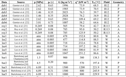
evaluation, experiment bar5 was also simulated and the axial distribution of the cross-482
sectional averaged void fraction is shown in Figure 2. In this case, the difference between the 483
simulation results is more marked, with lower coalescence in the flow causing a lower 484
average void fraction, probably as a consequence of the higher condensation. The 485
condensation heat transfer coefficient is indeed inversely proportional to the bubble diameter. 486
In view of these results, Wecrit = 1.24 was selected for the following simulations.
487
488
489
Figure 1. SMD and void fraction radial profiles compared against experiments deb1 (a,b) and 490
deb2 (c,d) and for different values of Wecritin the coalescence model: () 1.24; (---) 0.1.
491
493 494
495
Figure 2. Average void fraction axial development compared against experiment bar5 and for 496
different values of Wecrit in the coalescence model: () 1.24; (---) 0.1.
497
498
4.2 Bubble departure diameter
499 500
In preliminary simulations, it was found impossible to use, in the boiling model, the same set 501
of closure relations to address the entire database, in particular for the active nucleation site 502
density and the bubble departure diameter. For the nucleation site density, the Hibiki and Ishii 503
model [30] was maintained for the entire database because it accounts for the effect of more 504
parameters. Due to the fact that the database extends from atmospheric pressure up to 6.89 505
MPa, the Kocamustafaogullari model [32] was initially considered for the bubble departure 506
diameter, this being derived over the range 0.0067 < p < 14.18 MPa. In contrast, the 507
Tolubinsky and Kostanchuck [31] correlation was derived for 0.1 < p < 1.013 MPa and 0.08 508
< Ul < 0.20 m s-1 and has a pressure insensitive formulation, with the bubble departure
509
diameter being only a function of the bulk subcooling. Unfortunately, using the 510
Kocamustafaogullari correlation [32], reliable results were not obtained for the Roy et al. [21] 511
[image:19.595.192.393.102.300.2]data and the experiments of Bartolomej and co-authors [24,25]. An example is provided in 512
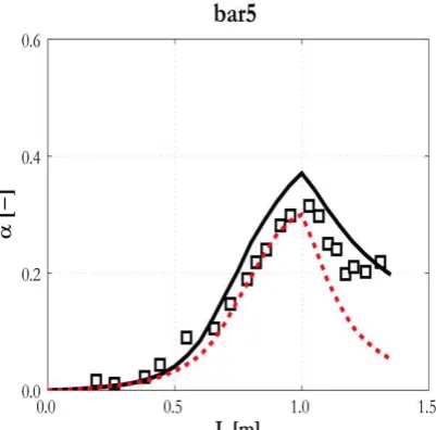
Figure 3, which shows predictions of the void distribution given by this correlation for the 513
bar2 (Figure 3b) and the bar4 (Figure 3d) experiments and compares these with the results 514
obtained using the Tolubinsky and Kostanchuk [31] correlation (Figure 3a and Figure 3c, 515
respectively). In the figure, r/R = 0.0 corresponds to the pipe axis and r/R = 1.0 to the pipe 516
wall. For bar2, at 4.5 MPa, Kocamustafaogullari [32] predicts a void fraction that is 517
MPa), however, the void fraction predicted with Kocamustafaogullari [32] is almost 519
negligible, except for a very thin portion of the wall region. Therefore, due to the negligible 520
evaporation predicted in some of the experiments, for the data of Bartolomej and Chanturiya 521
[24], Bartolomej et al. [25] and Roy et al. [21], the Tolubinsky and Kostanchuk [31] 522
correlation was used. 523
To investigate the subject further, some bubble departure diameter data selected from the 524
literature was tested against the Kocamustafaogullari model [32]. These data were taken from 525
Unal et al. [66] for water at high pressure, and from Klausner et al. [67] and Zeng et al. [68] 526
who used refrigerant R113, as employed by Roy et al. [21], at atmospheric pressure. 527
Percentage relative errors between predictions and data are shown in Figure 4. In general, the 528
bubble departure diameter is under predicted. More specifically, 50 – 75 % smaller diameters 529
are found for refrigerant R113 and, for water, the departure diameter is overestimated at low 530
pressure, but under predicted by up to 100% at high pressure. Overall, the relative percentage 531
errors are rather high, therefore the model cannot be considered reliable over a wide range of 532
conditions. 533
In line with the approach of the paper, it would have been desirable to maintain the 534
Tolubinsky and Kostanchuk [31] correlation for the whole database. However, this 535
correlation is also not entirely reliable even given its range of validity, as it was found that 536
unrealistically large bubbles were predicted by it for some of the Lee et al. [13] and the 537
DEBORA [22] experiments at low pressure, which prevented convergence of the simulations. 538
Therefore, for these two databases, the Kocamustafaogullari [32] correlation was used. 539
540
542
Figure 3. Void fraction radial distribution along the pipe for bar2 and bar4 experiments: 543
(a,c) Tolubinsky and Kostanchuk [31] bubble departure diameter correlation; (b,d) 544
Kocamustafaogullari [32] bubble departure diameter correlation. 545
546
547
[image:21.595.91.523.455.650.2]548
Figure 4. Relative percentage error for the Kocamustafaogullari [32] bubble departure 549
diameter correlation compared against: (a) Klausner et al. [67] and Zeng et al. [68] for 550
refrigerant R113; (b) Unal et al. [66] for water at different pressures. 551
552 553 554
4.3 Comparison with the entire database
555 556
After the preliminary selection of some of the model parameters, the overall model was 557
applied to the whole database without further modification. Comparisons for the DEBORA 558
experiments are presented in Figure 5 and Figure 6, and in Figure 7 for Roy et al. [21], in 559
Figure 8 for Lee et al. [13] and in Figure 9 for Batolomej and Chanturiya [24] and Bartolomej 560
et al. [25]. In these, and subsequent figures, symbols are used for experimental data and lines 561
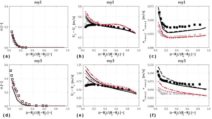
for model predictions. In annular channels (Figure 7 and Figure 8), the radial position is non-562
dimensionalized with the distance between the outer and inner radius and, therefore, in the 563
plots (r - Ri) / (Ro – Ri) = 0.0 identifies the inner wall, whereas (r - Ri) / (Ro – Ri) = 1.0
564
corresponds to the outer wall. Only the inner wall is heated in both the Roy et al. [14] and the 565
Lee et al. [13] experiments. In the following, discussion of the results is presented for each 566
physical quantity predicted. 567
568
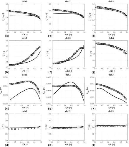
4.3.1 Void fraction
569
Even if the specific quantitative accuracy depends on the particular experiment, the void 570
fraction profile is generally predicted with reasonable accuracy. More specifically, the 571
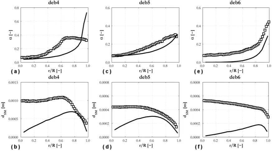
accuracy is satisfactory for the DEBORA experiment (Figure 5 and Figure 6), but with the 572
exception of deb6 (Figure 6c) where the void profile is significantly under predicted. Also, an 573
over predicted void peak at the heated wall was obtained for deb4 (Figure 6a). For deb3, it 574
must be remarked that the void fraction profile (Figure 5j) is core-peaked and the bubble 575
diameter (Figure 5k) higher than in all the other experiments. It is known from the literature 576
that larger bubbles assume ellipsoidal shapes, being deformed by the inertia of the 577
surrounding liquid, and are pushed towards the centre of the pipe by a negative lift force [45]. 578
In this experiment, bubbles may have been large enough to trigger the change of sign in the 579
lift force and, even if wall-peaked void profiles were predicted neglecting the lift 580
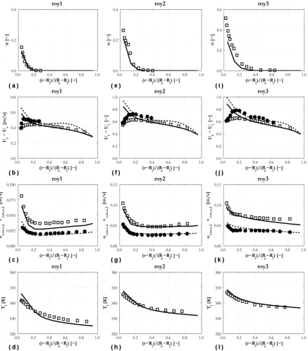
contribution, a negative lift was necessary to predict the void profile. In Figure 7, void 581
fraction profiles are well predicted for Roy et al. [21], the only discrepancy being a minor 582
underestimation in the case of roy3. In contrast, the void fraction tends to be underestimated 583
in the experiments of Lee et al. [13] (Figure 8). More specifically, the predicted void fraction 584
is in agreement with experiment or over predicted near the wall, whereas it is underestimated 585
in the remainder of the pipe. The best results are obtained at the lowest mass flux (lee1 in 586
Figure 8a and lee2 in Figure 8c), and the largest errors in lee5 (Figure 8i). Lastly, in the 587
was available and this is well predicted for bar1 and bar2 (Figure 9a), apart from a divergence 589
at around 1.25 m in bar2. Reasonable agreement is found for the Bartolomej et al. [25] 590
experiments in Figure 9b, despite the slight over prediction in bar3 and bar5. 591
592
4.3.2 Sauter-mean diameter
593
Measurements of the SMD were available for the DEBORA experiments only. Overall, the 594
model under predicts the experiments, in particular near the centre of the pipe, although 595
reasonable agreement is achieved for experiments deb2 (Figure 5g) and deb3 (Figure 5k), 596
whereas the under prediction is particularly large in deb6 (Figure 6e). In more detail, the 597
SMD is underestimated close to the heated wall and, after a partial improvement in the first 598
region away from the wall, predictions decrease significantly towards the pipe axis. In 599
contrast, the experimental profiles tend to remain nearly flat towards the centre of the pipe. In 600
deb3 (Figure 5k), the SMD increases towards the pipe centre, most likely as a consequence of 601
the core-peaked void fraction profile in this experiment, a trend that is also predicted by the 602
simulation. Overall, the significant discrepancies with the experiments may be due to a 603
number of different factors, the individual impact of which is difficult to quantify. Certainly, 604
the interphase heat transfer coefficient and the models for coalescence and break-up may play 605
a role that needs to be investigated further. In addition, the underestimation of the SMD in the 606
wall region suggests a significant impact of the bubble departure diameter correlation. This, 607
in conjunction with the unreliability of each bubble departure correlation over a wide range of 608
conditions, discussed in Section 4.2, demonstrates how the development of more advanced, 609
mechanistic formulations of the bubble departure diameter is a priority for further research. 610
4.3.3Liquid temperature
612
Liquid temperature profiles were measured by Roy et al. [21] and in the DEBORA 613
experiments. Overall, predictions are in good agreement with data. For the DEBORA 614
experiments, the flat temperature profile for deb2 (Figure 5h) and deb3 (Figure 5l) indicates 615
a flow close to saturation that may have helped to limit the underestimation of the SMD for 616
these experiments (Figure 5g and Figure 5k). deb1 (Figure 5d), instead, shows a slightly 617
higher degree of subcooling near the axis. The Roy et al. [21] experiments (Figure 7d, 618
Figure 7h and Figure 7l), which exhibit a higher degree of subcooling away from the wall, 619
are also well predicted, despite the temperature being slightly over estimated close to the 620
wall and under estimated near the axis. 621
622
4.3.4Velocity profiles
623
Liquid and vapour average velocities were measured by Roy et al. [21] and Lee et al. [13], 624
whereas only the average vapour velocity profile is available for the DEBORA 625
experiments. The vapour velocity profile is very well predicted for deb3 (Figure 5i), 626
although for deb1 (Figure 5a) and deb2 (Figure 5e), the profile remains flat near the pipe 627
centre, probably as a consequence of the lower value of the SMD in this region. However, 628
predictions may be considered satisfactory for these pipe flows. On the other hand, the 629
predicted accuracy is unsatisfactory in the annular channels of Roy et al. [21] and Lee et al. 630
[13]. More specifically, both predicted velocity profiles show a peak at the wall that is in 631
contrast found away from the wall in the experiments (Figure 7b, Figure 7f, Figure 7j, 632
Figure 8b, Figure 8d, Figure 8f, Figure 8h, Figure 8j and Figure 8l). This phenomenon is 633
even more evident in the vapour velocity profiles. Away from the wall, in particular for 634
Roy et al. [21], the velocity profiles are more in agreement with the experiments. The peak 635
away from the wall is explained due to the presence, in this region, of larger bubbles that 636
flow with a higher relative velocity. In Lee et al. [13], probably as a consequence of the 637
atmospheric pressure that promotes the growth of even larger bubbles, these peaks are 638
sometimes found in the “unheated half” of the channel. In the simulations, however, the 639
SMD peaks at the wall and the model is unable to correctly account for the presence of the 640
larger bubbles, with this inability also contributing to the low SMD values and the flat 641
velocity profiles in the centre of the channel predicted in deb1 (Figure 5a) and deb2 (Figure 642
5e). 643
644
4.3.5 Turbulence
645
Turbulence was only measured by Roy et al. [21] and the streamwise and radial r.m.s. of the 646
liquid velocity fluctuations are shown in Figure 7c, Figure 7g and Figure 7k. Overall, 647
turbulence is well predicted except for the under predicted streamwise r.m.s. in roy1 (Figure 648
7c). Also, the anisotropy of the turbulence field is reasonably well predicted by the Reynolds 649
stress turbulence model. 650
One of the advantages of building such a large database is the opportunity it affords to test 651
any model for all the variables of interest. However, and in view of the present results that 652
show the strengths of the model in some areas but weaknesses in others, measurements of all 653
the variables of interest in the same experiment are essential to further progress in the 654
modelling of boiling flows. 655
657
Figure 5. Average vapour velocity, void fraction, SMD and liquid temperature radial profiles 658
compared against the DEBORA experiments: (a-d) deb1; (e-h) deb2; (i-l) deb3. 659
661
Figure 6. Void fraction and SMD radial profiles compared against the DEBORA 662
experiments: (a-b) deb4; (c-d) deb5; (e-f) deb6. 663
665
Figure 7. Void fraction, liquid (, ) and vapour (---, ) average velocity, streamwise (, ) 666
and radial (---, ) r.m.s. of liquid velocity fluctuations and liquid temperature radial profiles 667
compared against Roy et al. [21]: (a-d) roy1; (e-h) roy2; (i-l) roy3. 668
671
Figure 8. Void fraction and liquid (, ) and vapour (---, ) average velocity radial profiles 672
compared against Lee et al. [13]: (a,b) lee1; (c,d) lee2; (e,f) lee3; (g,h) lee4; (i,j) lee5; (k,l) 673
lee6. 674
678
Figure 9. Average void fraction axial development compared against: (a) Bartolomej and 679
Chanturiya [24]; (b) Bartolomej et al. [25]. (a): (, ) bar1; , ) bar2. (b): (, ) bar3; (---680
, ) bar4; (--,∆) bar5. 681
682
4.4 Near-wall treatment
683 684
In the previous section, the most significant deviations from experiments were found for the 685
average velocity profiles in the near-wall region of annular channels. In the last 686
computational cell close to the wall, the velocity boundary condition is imposed through the 687
use of wall functions, with the standard single-phase wall function having been used in the 688
simulations. Some authors [8,9,69] have demonstrated how predictions in the near-wall 689
region can be improved with the adoption of a simple wall roughness model, similar to those 690
used in turbulent flows over rough surfaces, but with the equivalent roughness equal to the 691
bubble departure diameter. To the authors’ knowledge, such a modification has yet to be 692
tested with an RSM turbulence model. In a first set of simulations with the RSM, it was 693
found difficult to reach convergence and handle the rather high wall roughness values (equal 694
to the bubble departure diameter). Therefore, the wall roughness model was tested using a k- 695
formulation. The results are reported in Figure 10 for experiments roy2, roy3 and lee2, and, 696
for the k- model with the standard wall function, these show the same features discussed for 697
the RSM, i.e. liquid and vapour average velocity profiles show the same peak at the wall and 698
rather high values with respect to the experiments. 699
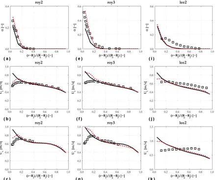
For the lower void fraction cases (roy2 and lee2), agreement for the liquid velocity improves 700
and the profile peaks at a certain distance from the wall with inclusion of the wall roughness 701
for the vapour velocity profile (Figure 10c). In the highest void fraction experiment (roy3), 703
the improvement is also marginal for the liquid velocity (Figure 10f and Figure 10g). In roy2 704
and roy3, the wall roughness model also produces an increase in the void fraction (Figure 10a 705
and Figure 10e), although this remains unchanged in lee2 (Figure 10i). 706
Overall, the introduction of the wall roughness model is seen to improve the predictions, 707
although the improvements noted are not significant in all cases examined. In addition to 708
further development of the wall model and its extension for use with RSM, it also seems 709
necessary, based on the discussion in Section 4.3.4, to better account for the behaviour of 710
larger bubbles, extending to boiling flows recently developed population balance models that 711
account for their behaviour separately [10,65]. 712
713
[image:31.595.80.519.298.666.2]714
Figure 10. Void fraction and average liquid and vapour velocity radial profiles compared 715
against Roy et al. [21] and Lee et al. [13]: (a-c) roy1; (e-g) roy2; (i-k) roy3. () standard 716
wall function; (---) wall roughness model [8]. 717
4.5 Bubble-induced turbulence
719 720
It has been established how, in bubbly flows, the bubbles contribute to the turbulence of the 721
continuous phase and this contribution must be accounted for in the turbulence model 722
[48,54,60]. Many studies have been conducted on the subject, but only a few of them have 723
focused on boiling flows, and, therefore, the impact of the bubble contribution on the 724
turbulence is much more uncertain in these flows. In Section 4.3.5, the bubble-induced 725
contribution was neglected. Nevertheless, turbulence in the continuous phase was well 726
predicted, even if measurements were available only for Roy et al. [21] (Figure 7c, Figure 7g 727
and Figure 7k). This may suggest that bubble-induced turbulence is less important with 728
respect to adiabatic bubbly flows even if it must be noticed that, in Roy et al. [21], the void 729
fraction is very low or zero in the majority of the channel (Figure 7a, Figure 7e and Figure 730
7i). Also, in the regions of high void fraction close to the wall, this influence is further 731
complicated with respect to adiabatic bubbly flows due to the detachment into the bulk fluid 732
of bubbles growing on the heated wall. 733
The roy1 and roy3 calculations were repeated with the bubble-induced turbulence model (Eq. 734
(4) and Eq. (5)) and the results are shown in Figure 11. In roy1, the r.m.s. values are changed 735
only in the region very close to the wall (Figure 11c), where the velocity fluctuations are now 736
overestimated. The same effect is obtained for roy3 and for a larger portion of the pipe 737
section (Figure 11f). Therefore, the model accuracy is generally worsened with inclusion of 738
the bubble-induced turbulence model. Void fraction (Figure 11a and Figure 11d) and average 739
velocity (Figure 11b and Figure 11e) predictions are also increased relative to those without 740
the bubble-induced turbulence contribution. The findings are, however, complicated by the 741
fact that, due to the peak in the velocity profiles, the shear-induced turbulence close to the 742
wall may also be overestimated and this may be the reason for the overestimation of 743
turbulence levels when the bubble-induced contribution is accounted for. More studies are 744
necessary on this subject, but, since bubbles detachment occurs in the first computational cell 745
close to the wall, and in view of the results from the previous section on the wall treatment, it 746
is suggested that the problem needs to be approached globally, addressing jointly in the same 747
model the velocity boundary condition and the generation of turbulence close to the wall, as 748
well as the contribution from the bubbles in this region. 749
751
Figure 11 Void fraction, liquid ( ,,) and vapour ( ,---,--) average velocity and 752
streamwise ( ,,) and radial ( ,---,--) r.m.s. of the liquid velocity fluctuations radial 753
profiles compared against Roy et al. [21]: (a-c) roy1; (d-f) roy3. (,---) without bubble 754
induced turbulence model; (,--) with bubble induced turbulence model. 755
756
5
Conclusions
757 758
An Eulerian-Eulerian two-fluid CFD model, including a Reynolds stress turbulence model, 759
the method of moments-based S population balance approach and a boiling model derived
760
from the RPI heat flux partitioning approach, was used to predict a large database of 761
subcooled boiling flows. The database includes 20 experiments of subcooled boiling flows of 762
water and refrigerants in vertical pipes and annular channels, and covers a wide range of 763
conditions. 764
Overall, the model confirms the potential of CFD to provide detailed predictions of boiling 765
flows and rather good agreement with data was found in some areas, but others still require 766
significant improvements in model accuracy. At the present time, the general applicability of 767
the model is not entirely satisfactory. Even if built in a mechanistic fashion, numerous 768
empirical closure relations are required, not only for wall boiling, but also for the population 769
balance and turbulence models. This clearly limits the overall model’s general applicability 770
and, therefore, the development of more mechanistic closures is highly desirable. A good 771
example is provided by the bubble departure diameter that cannot be predicted with accuracy 772
of physically-based, more accurate closure models is challenging and may only be achieved 774
with an increase in our knowledge of mechanisms that are as yet not completely understood, 775
such as the growth and departure of bubbles, but also their breakup and coalescence and the 776
interaction of turbulence with bubbles near the wall, amongst others. 777
The results show how studies such as the one described, which focused on a large database, 778
can profitably be used to integrate detailed analyses based on more limited amounts of data. 779
In the latter, major developments of specific sub-models can be derived and tested, but these 780
developments can only be accepted if they improve the general accuracy of models when 781
tested against large sets of data. The disparity observed between individual experiments 782
suggests that it is risky to judge the accuracy of any CFD model on the basis of a limited 783
number of comparisons with data. 784
Quantitatively, the predictive accuracy is satisfactory for the void fraction, except for a 785
limited number of cases, with the turbulence and liquid temperature fields also well 786
predicted. In contrast, the average bubble diameter, quantified by the SMD, tends to be 787
underestimated, sometimes significantly, in particular near the axis of the flows, with velocity 788
profiles also over predicted near the heated wall of annular channels, where they exhibit a 789
peak that is instead found away from the wall in the experiments. 790
Despite the inaccuracy of some predictions, the satisfactory results achieved in some areas 791
encourage further research: 792
No correlation for the bubble departure diameter was found appropriate for the entire 793
database and the under prediction of the departure diameter was identified as a 794
possible source of error in the average bubble diameter predictions. The use of more 795
mechanistic formulations, already adopted by a limited number of researchers, 796
represents a way forward in this regard. 797
Modelling of bubble break-up and coalescence needs to be improved, with related
798
improvements in population balance modelling also required. More specifically, the 799
ability to account for larger bubbles moving towards the flow centre, already available 800
for adiabatic flows, may improve the prediction of velocity profiles in both pipes and 801
channels. 802
Velocity predictions near the wall were improved using a wall roughness model, but
803
further development is required, in particular in the context of RSM. 804
Bubble-induced turbulence was demonstrated to be less relevant with respect to
805
advanced modelling approach seems necessary near the wall, but it should be 807
addressed together with the wall treatment. 808
809
Acknowledgements
810 811
The authors gratefully acknowledge the financial support of the EPSRC under grant 812
EP/K007777/1, Thermal Hydraulics for Boiling and Passive Systems, part of the UK-India 813
Civil Nuclear Collaboration. 814
815
Nomenclature
816
Ab fraction of the wall affected by the evaporation process [m-1]
817
ai interfacial area concentration [m2 m-3]
818
CD drag coefficient [-]
819
Cp specific thermal capacity at constant pressure [J kg-1 K-1]
820
D diameter [m]
821
dB bubble diameter [m]
822
dcrit critical bubble diameter [m]
823
dSM Sauter mean diameter [m]
824
dw bubble departure diameter [m]
825
Eo bubble Eotvos number Eo = g ( l – v) dB2 / [-]
826
Fd drag force [N m-3]
827
FTD turbulent dispersion force [N m-3]
828
f frequency of bubble departure [s-1]
829
G mass flux [kg m-2s-1]
830
g gravitational acceleration [m s-2]
831
hq quenching heat transfer coefficient [W m-3K-1]
832
ilv latent heat of vaporization [J kg-1]
833
Kbr break-up rate [s-1]
834
Kcld,d’ coalescence rate [s-1]
835
Kdry fraction of the heated wall in contact with the vapour phase [-]
836
k turbulence kinetic energy [m2s-2]
837
L pipe/channel length [m]
838
M th moment of the bubble diameter distribution [m ]
839
mlv interphase mass transfer [kg m-3s-1]
840
N bubble generation rate per unit volume [bubbles m-3s-1]
Nf number of daughter bubbles [-]
842
n bubble number density [bubbles m-3]
843
n’ nucleation site density [m-2]
844
P(dB) bubble diameter probability distribution [-]
845
Pr Prandtl number Pr = Cp / k [-]
846
p pressure [Pa]
847
pr reduced pressure p/pcrit [-]
848
Qev evaporative volumetric heat flux [W m-3]
849
Ql liquid phase convective volumetric heat flux [W m-3]
850
Qq quenching volumetric heat flux [W m-3]
851
Qv vapour phase convective volumetric heat flux [W m-3]
852
Qw total wall volumetric heat flux [W m-3]
853
q" heat flux [W m-2K-1] 854
R radius [m]
855
Rg gas constant [J mol-1K-1]
856
Rij Reynolds stress [m2s-2]
857
r radial coordinate [m]
858
Re bubble Reynolds number Re = l Ur dB / l [-]
859
Sbr source of S due to bubble break-up [m m-3s-1]
860
Scl source of S due to bubble coalescence [m m-3s-1]
861
Sm source of S due to boiling and evaporation [m m-3s-1]
862
SkBI bubble-induced turbulence kinetic energy source [kg m s-3]
863
SBI bubble-induced turbulence energy dissipation rate source [kg m s-4]
864
S density of the th moment of the bubble diameter distribution [m m-3]
865
∆Sbr change in S due to a single break-up event [m ]
866
change in S due to a single coalescence event [m ] 867
T temperature [°C]
868
T+ dimensionless temperature [-]
869
t time [s]
870
tw waiting time for bubble departure [s]
871
U velocity [m s-1]
872
ur.m.s. streamwise r.m.s. of the velocity fluctuations [m s-1]
873
vr.m.s. radial r.m.s. of the velocity fluctuations [m s-1]

![Figure 3. Void fraction radial distribution along the pipe for bar2 and bar4 experiments: (a,c) Tolubinsky and Kostanchuk [31] bubble departure diameter correlation; (b,d) Kocamustafaogullari [32] bubble departure diameter correlation](https://thumb-us.123doks.com/thumbv2/123dok_us/7824231.173954/21.595.90.523.74.348/distribution-experiments-tolubinsky-kostanchuk-departure-correlation-kocamustafaogullari-correlation.webp)