Multiple time-dependent coefficient identification thermal problems with a free boundary

This is a repository copy of Multiple time-dependent coefficient identification thermal problems with a free boundary.

White Rose Research Online URL for this paper: http://eprints.whiterose.ac.uk/89650/

Version: Accepted Version

Article:

Hussein, MS, Lesnic, D, Ivanchov, MI et al. (1 more author) (2016) Multiple

time-dependent coefficient identification thermal problems with a free boundary. Applied Numerical Mathematics, 99. 24 - 50. ISSN 0168-9274

https://doi.org/10.1016/j.apnum.2015.09.001

© 2015, Elsevier. Licensed under the Creative Commons Attribution-NonCommercial-NoDerivatives 4.0 International http://creativecommons.org/licenses/by-nc-nd/4.0/

[email protected] https://eprints.whiterose.ac.uk/

Reuse

Unless indicated otherwise, fulltext items are protected by copyright with all rights reserved. The copyright exception in section 29 of the Copyright, Designs and Patents Act 1988 allows the making of a single copy solely for the purpose of non-commercial research or private study within the limits of fair dealing. The publisher or other rights-holder may allow further reproduction and re-use of this version - refer to the White Rose Research Online record for this item. Where records identify the publisher as the copyright holder, users can verify any specific terms of use on the publisher’s website.

Takedown

If you consider content in White Rose Research Online to be in breach of UK law, please notify us by

Multiple time-dependent coefficient identification

thermal problems with a free boundary

M.S. Hussein1,2_{, D. Lesnic}1_{, M.I. Ivanchov}3 _{and H.A. Snitko}4

1_{Department of Applied Mathematics, University of Leeds, Leeds LS2 9JT, UK}

2_{Department of Mathematics, College of Science, University of Baghdad, Baghdad, Iraq} 3_{Faculty of Mechanics and Mathematics, Department of Differential Equations, Ivan Franko} National University of Lviv, 1, Universytetska str., Lviv, 79000, Ukraine

4_{Pidstryhach Institute for Applied Problems of Mechanics and Mathematics of National} Academy of Science of Ukraine, 3-b, Naukova Str., Lviv, 79060, Ukraine

E-mails: [email protected] (M.S. Hussein), [email protected] (D. Lesnic), [email protected] (M.I. Ivanchov), [email protected] (H.A. Snitko).

Abstract

Multiple time-dependent coefficient identification thermal problems with an unknown free boundary are investigated. The difficulty in solving such inverse and ill-posed free boundary problems is amplified by the fact that several quantities of physical interest (conduction, convection/advection and reaction coefficients) have to be simultaneously identified. The additional measurements which render a unique solution are given by the heat moments of various orders together with a Stefan boundary condition on the unknown moving boundary. Existence and uniqueness theorems are provided. The nonlinear and ill-posed problems are numerically discretised using the finite-difference method and the resulting system of equa-tions is solved numerically using the MATLAB toolbox routine lsqnonlin applied to mini-mizing the nonlinear Tikhonov regularization functional subject to simple physical bounds on the variables. Numerically obtained results from some typical test examples are presented and discussed in order to illustrate the efficiency of the computational methodology adopted.

Keywords: Inverse problem; Tikhonov regularization; Free boundary; Heat equation.

1

Introduction

Inverse coefficient identification problems (ICIP) for partial differential equations are some of the most complicated and practically important problems. Being in addition nonlinear, optimization techniques are mainly used for their numerical solutions, as well as various modifications tailored to the properties of the corresponding direct problems (monotonicity or/and smoothness of their solutions, etc.), [13]. ICIP’s with one or several unknown coef-ficients play a substantial role in the theory and application of inverse problems. A great attention was paid to this kind of inverse problems due to the industrial applications in prac-tice, for instance, the determination of the thermal conductivity, heat capacity, absorption coefficient, etc., in the field of heat conduction or porous media.

Prior to this study, references [4, 6, 10] investigated both theoretically and numerically several such combined formulations for the retrieval of the free boundary together with the thermal diffusivity both which are unknown time-dependent functions. The theoretical investigation has been extended recently to the case of several multiple coefficients in [18, 19] and it the purpose of this study to, apart from some theoretical clarifications which are elaborated in Section 2, perform the numerical realization using the finite-difference method (FDM) combined with a nonlinear least-squares toolbox MATLAB routine, see Sections 3 and 4. In Section 5, we provide numerical results and discussion, whilst Section 6 presents an extension to a triple unknown coefficient identification. Finally, conclusions are highlighted in Section 7.

2

Mathematical formulation

Consider the one-dimensional time-dependent heat equation

∂u

∂t(x, t) =a(x, t) ∂2_u

∂x2(x, t) +b(t)

∂u

∂x(x, t) +c(t)u(x, t) +f(x, t), (x, t)∈Ω (1) for the unknown temperature u(x, t) in the domain Ω = _{(x, t)_| 0 < x < h(t),0 < t <

T <_∞} with unknown free smooth boundary x=h(t)>0 and time-dependent coefficients

b(t) and c(t) representing the convection/advection and reaction coefficients, respectively. Also in (1), f(x, t) represents a given heat source, whilst a(x, t) > 0 is the given thermal diffusivity. In many applications, [6, 19, 24], the thermal diffusivity depends on time only, but here we envisage a more general physical situation in which the thermal conductivity depends on time and the heat capacity depends on space such that their ratio defined as the thermal diffusivity depends on both space and time. To give more physical meaning to the inverse problem, we have in mind a process in which a finite slab is undertaking radioactive decay such that its diffusivity, convection and reaction coefficients are unknown but they depend on time [1, Chap.13], [16]. We finally mention that extensions to cases when the time-dependent heat source is also unknown or when some unknown coefficients may depend on space as well have recently been considered elsewhere, [7, 8].

The initial condition is

u(x,0) =ϕ(x), 0_≤x_≤h(0) =:h0, (2)

whereh0 >0 is given, and the Dirichlet boundary conditions are

u(0, t) =µ1(t), u(h(t), t) =µ2(t), t ∈[0, T]. (3)

As over-determination conditions we consider, [18],

h′_{(t) +u}

x(h(t), t) =µ3(t), t ∈[0, T], (4)

∫ h(t)

0

u(x, t)dx=µ4(t), t ∈[0, T], (5)

∫ h(t)

0

xu(x, t)dx=µ5(t), t ∈[0, T]. (6)

Note that µ4(t) and µ5(t) represent the specification of the energy or, mass of the heat

Now we perform the change of variabley =x/h(t) to reduce the problem (1)–(6) to the following inverse problem for the unknownsh(t),b(t),c(t) and v(y, t) := u(yh(t), t):

∂v

∂t(y, t) =

a(yh(t), t) h2_(t)

∂2_v

∂y2(y, t) +

b(t) +yh′_(t) h(t)

∂v

∂y(y, t) +c(t)v(y, t)+f(yh(t), t),

(y, t)_∈QT (7)

in the fixed domainQT :={(y, t) : 0< y < 1,0< t < T}= (0,1)×(0, T),

v(y,0) =ϕ(h0y), y∈[0,1], (8)

v(0, t) =µ1(t), v(1, t) =µ2(t), t ∈[0, T], (9)

h′_{(t) +} 1

h(t)vy(1, t) =µ3(t), t∈[0, T], (10)

h(t)

∫ 1

0

v(y, t)dy=µ4(t), t∈[0, T], (11)

h2(t)

∫ 1

0

yv(y, t)dy=µ5(t), t∈[0, T]. (12)

A variant of the theorem proved in [18] (under the additional assumption thath(0) =h0 >0

is known) ensures the unique solvability (locally in time) of the inverse problem (7)–(12), as follows.

Theorem 1. Suppose that:

0 < a _∈ C2,0_{([0,∞)×[0, T]), [0, f}

0] ∋ f ∈ C1,0([0,∞)×[0, T]), where f0 ≥ 0 is a given constant, 0< ϕ_∈C1_{[0, h}

0], 0< µi ∈C1[0, T] for i= 1,2,4,5, µ3 ∈C[0, T],

(µ2(0)−µ1(0))µ5(0)−(h0µ2(0)−µ4(0))µ4(0)̸= 0, (13)

ϕ(0) = µ1(0), ϕ(h0) = µ2(0),

∫h0

0 ϕ(x)dx = µ4(0), and

∫h0

0 xϕ(x)dx = µ5(0). Then, there is T0 ∈ (0, T], such that there exists a unique solution (h(t), b(t), c(t), v(y, t)) ∈ C1[0, T0]×

(C[0, T0])2×(C2,1(QT0)∩C 1,0_(Q

T0)),h(t)>0fort ∈[0, T0], of the inverse problem (7)–(12).

Remarks.

(i) During the computation we need the values ofb(0) andc(0). One can derive these values from the governing equation (1) with the help of overdetermination conditions (5) and (6), as follows. Integrating (1) with respect tox over the interval [0, h(t)] we have

∫ h(t)

0

ut(x, t)dx=a(h(t), t)ux(h(t), t)−a(0, t)ux(0, t)−

∫ h(t)

0

ax(x, t)ux(x, t)dx

+b(t)(µ2(t)−µ1(t)) +c(t)µ4(t) +

∫ h(t)

0

f(x, t)dx. (14)

Also, multiplying (1) byx and integrating with respect to x over the interval [0, h(t)], and invoking the integration by parts, we obtain

∫ h(t)

0

xut(x, t)dx=h(t)a(h(t), t)ux(h(t), t)−

∫ h(t)

0

(a(x, t) +xax(x, t))ux(x, t)dx

+b(t)(h(t)µ2(t)−µ4(t)) +c(t)µ5(t) +

∫ h(t)

0

Differentiating equations (5) and (6) with respect tot we obtain

∫ h(t)

0

ut(x, t)dx=µ′4(t)−h′(t)µ2(t),

∫ h(t)

0

xut(x, t)dx=µ′5(t)−h(t)h′(t)µ2(t). (16)

Substituting (16) into (14) and (15) and usingy=x/h(t) we obtain

b(t)(µ2(t)−µ1(t)) +c(t)µ4(t) =µ′4(t)−µ2(t)h′(t) +

a(0, t)w(0, t)₋a(h(t), t)w(1, t) h(t)

+

∫ 1

0

ax(yh(t), t)w(y, t)dy−h(t)

∫ 1

0

f(yh(t), t)dy, (17)

b(t)(h(t)µ2(t)−µ4(t)) +c(t)µ5(t) =µ′5(t)−µ2(t)h(t)h′(t)−a(h(t), t)w(1, t)

+

∫ 1

0

(

a(yh(t), t) +yh(t)ax(yh(t), t)

)

w(y, t)dy₋h2(t)

∫ 1

0

yf(yh(t), t)dy, (18)

where we have denotedw(y, t) := vy(y, t). Equation (10) also gives

h′_{(t) =−}w(1, t)

h(t) +µ3(t), t∈[0, T]. (19)

Substituting this expression into (17) and (18) and solving the resulting system of equations forb(t) and c(t), result in equations (18) and (19) (corrected) of [18], namely,

b(t) = 1

D1(t)

{ ∫ 1

0

[

(µ5(t)−yh(t)µ4(t))ax(yh(t), t)−a(yh(t), t)µ4(t)

]

w(y, t)dy

+a(0, t)µ5(t)

h(t) w(0, t) +

(µ2(t)−a(h(t), t))(µ5(t)−h(t)µ4(t))

h(t) w(1, t)

−h(t)

∫ 1

0

(

µ5(t)−yh(t)µ4(t)

)

f(yh(t), t)dy+µ′

4(t)µ5(t)−µ4(t)µ′5(t)

−µ2(t)µ3(t)

(

µ5(t)−h(t)µ4(t)

) }

, t_∈[0, T], (20)

c(t) = 1

D1(t)

{ ∫ 1

0

[

(µ2(t)−µ1(t))a(yh(t), t) +

(

h(t)(µ2(t)(y−1)−yµ1(t))

+µ4(t)

)

ax(yh(t), t)

]

w(y, t)dy+ (µ4(t)−h(t)µ2(t))a(0, t)

h(t) w(0, t)

+(µ2(t)−a(h(t), t))(µ4(t)−h(t)µ1(t))

h(t) w(1, t)−h(t)µ2(t)

(

µ′

4(t)−µ1(t)µ3(t)

)

−h(t)

∫ 1

0

(

µ4(t) +h(t)

(

µ2(t)(y−1)−yµ1(t)

) )

f(yh(t), t)dy

+µ4(t)µ′4(t) +µ′5(t)(µ2(t)−µ1(t))−µ2(t)µ3(t)µ4(t)

}

, t_∈[0, T], (21)

where

D1(t) := (µ2(t)−µ1(t))µ5(t)−(h(t)µ2(t)−µ4(t))µ4(t), t∈[0, T]. (22)

One can observe that condition (13) of Theorem 1 is equivalent toD1(0)̸= 0, and since the

[0, T1] of t = 0, where T1 ∈ (0, T]. So, at least in this neighbourhood the denominator in

(20) and (21) does not vanish hence, these expressions are well-defined.

Letting t = 0 in the analogue of expressions (20) and (21) in the variable x, we obtain the values ofb(0) andc(0) explicitly, as follows:

b(0) = 1 D1(0)

[ ∫ h0

0

[

(µ5(0)−xµ4(0))ax(x,0)−a(x,0)µ4(0)

]

ϕ′_(x)dx

+a(0,0)µ5(0)ϕ′(0) + (µ2(0)−a(h0,0))(µ5(0)−h0µ4(0))ϕ′(h0)

−

∫ h0

0

(

µ5(0)−xµ4(0))f(x,0)dx+µ′4(0)µ5(0)−µ4(0)µ′5(0)

−µ2(0)µ3(0)

(

µ5(0)−h0µ4(0)

) ]

, (23)

c(0) = 1 D1(0)

[ ∫ h0

0

(

(µ2(0)−µ1(0))a(x,0) +

(

µ2(0)(x−h0)−xµ1(0)

+µ4(0)

)

ax(x,0)

)

ϕ′_{(x)dx+a(0,0)ϕ}′_(0)(µ

4(0)−h0µ2(0))

+ (µ2(0)−a(h0,0))(µ4(0)−h0µ1(0))ϕ′(h0)−h(0)µ2(0)

(

µ′

4(0)−µ1(0)µ3(0)

)

−

∫ h0

0

(

µ4(0) +µ2(0)(x−h0)−xµ1(0)

)

f(x,0)dx

+µ4(0)µ′4(0) +µ′5(0)(µ2(0)−µ1(0))−µ2(0)µ3(0)µ4(0)

]

. (24)

One can further elaborate on the determinant (22) of the system of equations (14) and (15), by rewriting it as follows:

D1(t) =

∫ h(t)

0

ux(x, t)dx

∫ h(t)

0

xu(x, t)dx₋

∫ h(t)

0

u(x, t)dx

∫ h(t)

0

xux(x, t)dx

=

∫ h(t)

0

∫ h(t)

0

(ξ₋x)u(ξ, t)ux(x, t)dxdξ. (25)

Let us divide the square (0, h(t))_×(0, h(t)) by its main diagonal and separate the integration in (25) into two parts. Then we obtain

D1(t) =−

∫ h(t)

0

dx

∫ x

0

(x₋ξ)u(ξ, t)ux(x, t)dξ+

∫ h(t)

0

dξ

∫ ξ

0

(ξ₋x)u(ξ, t)ux(x, t)dξ.

In the first integral change x byξ and ξ byx to obtain

D1(t) =−

∫ h(t)

0

uξ(ξ, t)dξ

∫ ξ

0

(ξ₋x)u(x, t)dx+

∫ h(t)

0

u(ξ, t)dξ

∫ ξ

0

(ξ₋x)ux(x, t)dx

=

∫ h(t)

0

dξ

∫ ξ

0

(ξ₋x)[

u(ξ, t)ux(x, t)−u(x, t)uξ(ξ, t)

]

dx

=

∫ h(t)

0

u(ξ, t)dξ

∫ ξ

0

(ξ₋x)u(x, t)

(

ux(x, t)

u(x, t) −

uξ(ξ, t)

u(ξ, t)

)

dx

=₋

∫ h(t)

0

u(ξ, t)dξ

∫ ξ

0

(ξ₋x)u(x, t)dx

∫ ξ

x

∂ ∂ζ

(

uζ(ζ, t)

u(ζ, t)

)

From conditionsϕ >0, µ1 >0,µ2 >0,f ≥0,a >0, it follows from the minimum principle

that

u(x, t)>0, (x, t)_∈Ω. (27)

The last derivative in (26) is given by

∂2

∂ζ2

(

lnu(ζ, t)

)

= ∂

∂ζ

(

uζ(ζ, t)

u(ζ, t)

)

= uζζ(ζ, t) u(ζ, t) −

u2 ζ(ζ, t)

u2_{(ζ, t)}. (28)

One can therefore make D1(t) ̸= 0 in (26) if, via (28), we have (lnu(ζ, t))ζζ ̸= 0. This last

inequality may be satisfied locally in time (in a neighborhood of t= 0) if ϕ _∈C2_{[0, h} 0] and

(lnϕ)′′ _{̸= 0.}

(ii) If we make the stronger assumption that ϕ _∈ C2_{[0, h}

0] then, there is a simpler way to

obtain b(0) and c(0) in terms of expressions that do not involve the heat moments µ4 and

µ5 by using the direct problem data (2) and (3) only. Indeed, if we put (x, t) = (0,0) and

(x, t) = (h0,0) into equation (1) we obtain

µ′

1(0) =a(0,0)ϕ′′(0) +b(0)ϕ′(0) +c(0)ϕ(0) +f(0,0),

µ′

2(0) =a(h0,0)ϕ′′(h0) +b(0)ϕ′(h0) +c(0)ϕ(h0) +f(h0,0).

}

(29)

Then, provided that ϕ′_(0)ϕ(h

0)−ϕ(0)ϕ′(h0)̸= 0, the solution of this system is given by

b(0) = ϕ(h0)(µ′1(0)−a(0,0)ϕ′′(0)−f(0,0))−ϕ(0)(µ′2(0)−a(h0,0)ϕ′′(h0)−f(h0,0))

ϕ′_{(0)ϕ(h0)−ϕ(0)ϕ}′_(h0) ,

(30)

c(0) = ϕ′(0)(µ′2(0)−a(h0,0)ϕ′′(h0)−f(h0,0))−ϕ′(h0)(µ′1(0)−a(0,0)ϕ′′(0)−f(0,0)) ϕ′_{(0)ϕ(h0)−ϕ(0)ϕ}′_(h0)

(31)

(iii) In [18], a stronger assumption than (13) was used. Namely, that

(µ2(t)−µ1(t))µ5(t)−(H1µ2(t)−µ4(t))µ4(t)>0, t∈[0, T], (32)

where

H1 =

2 max

t∈[0,T]µ4(t)

min_{ min

x∈[0,h0]

ϕ(x), min

t∈[0,T]µ1(t),tmin∈[0,T]µ2(t)}

. (33)

However, assumption (32) seems too restrictive and it is difficult to ensure in numerical experiments (with an analytical solution available). Whilst the less restrictive condition (13) still ensures the local unique solvability of the inverse problem. Furthermore, expressions (20) and (21) for b(t) and c(t), respectively, are well-defined if the function D1 defined in

(22), does not vanish on the interval [0, T].

2.1

Another related inverse problem formulation

It was pointed out in [18] that the Stefan condition (4), or (10), may be replaced by the second-order heat moment measurement

∫ h(t)

0

x2_{u(x, t)dx=µ}

6(t), t ∈[0, T], (34)

or, in terms of the variabley =x/h(t),

h3(t)

∫ 1

0

y2v(y, t)dy=µ6(t), t∈[0, T], (35)

respectively. Then, we can formulate the following theorem on the local unique solvability of the inverse problem (7)–(9), (11), (12) and (35), which is a variant of Theorem 2 of [18] whenh(0) =h0 >0 is assumed to be known.

Theorem 2. Suppose that:

0 < a _∈ C2,0_{([0,∞)×[0, T]), [0, f}

0] ∋ f ∈ C1,0([0,∞)×[0, T]), where f0 ≥ 0 is a given constant, 0< ϕ_∈C1_{[0, h}

0], 0< µi ∈C1[0, T] for i= 1,2,4,5,6,

µ4(0)µ6(0)−2µ25(0)−h0(µ6(0)µ1(0)−2µ4(0)µ5(0))−h20(µ24(0)−µ1(0)µ5(0))̸= 0, (36)

ϕ(0) =µ1(0), ϕ(h0) = µ2(0),

∫h0

0 ϕ(x)dx=µ4(0),

∫h0

0 xϕ(x)dx =µ5(0), and

∫h0

0 x2ϕ(x)dx = µ6(0). Then, there is T0 ∈ (0, T], such that there exists a unique solution

(h(t), b(t), c(t), v(y, t)) _∈ C1_{[0, T}

0]× (C[0, T0])2 ×(C2,1(QT0) ∩ C 1,0_(Q

T0)), h(t) > 0 for

t_∈[0, T0], of the inverse problem (7)–(9), (11), (12) and (35). Proof. Following [18], let us introduce the notations

p(t) :=h′_{(t), w(y, t) :=v}

y(y, t). (37)

Then, we can reduce the problem (7)–(9), (11), (12) and (35) to a system of integral equations for the unknowns h(t), p(t),b(t),c(t), v(y, t) and w(y, t), as follows.

First, let us denote by G1(y, t;η, τ) the Green function of the Dirichlet boundary-value

problem for the equation

∂V

∂t (y, t) =

a(yh(t), t) h2_(t)

∂2_V

∂y2(y, t).

Then,v(y, t) satisfying equations (7)–(9) can be represented in the form

v(y, t) = v0(y, t) +

∫ t

0

∫ 1

0

G1(y, t;η, τ)

((

b(τ) +ηp(τ) h(τ)

)

w(η, τ) +c(τ)v(η, τ)

)

dηdτ, (38)

wherev0(y, t) is given by, [11],

v0(y, t) =

∫ 1

0

G1(y, t;η,0)ϕ(h0η)dη+

∫ t

0

∂G1

∂η (y, t; 0, τ)

a(0, τ)

h2_(τ) µ1(τ)dτ

−

∫ t

0

∂G1

∂η (y, t; 1, τ)

a(h(τ), τ)

h2_(τ) µ2(τ)dτ+

∫ t

0

∫ 1

0

Let us now rewrite the problem (7)–(9) forv into a new one for the partial derivative vy

which was denoted by w in (37). For this, we differentiate with respect to y equations (7) and (8), apply (7) at y_{∈ {}0,1_} and use (9) to obtain

∂w

∂t(y, t) =

a(yh(t), t) h2_(t)

∂2_w

∂y2(y, t) +

(

ax(yh(t), t) +b(t) +yh′(t)

h(t)

)

∂w ∂y(y, t)

+

(

h′_(t)

h(t) +c(t)

)

w(y, t) +h(t)fx(yh(t), t), (y, t)∈QT, (40)

w(y,0) = h0ϕ′(h0y), y∈[0,1], (41)

∂w

∂y(0, t) = h2_(t)

a(0, t)

(

µ′

1(t)−

b(t)

h(t)w(0, t)−c(t)µ1(t)−f(0, t)

)

, t_∈[0, T], (42)

∂w

∂y(1, t) =

h2_(t)

a(h(t), t)

(

µ′

2(t)−

(

b(t) +h′_(t) h(t)

)

w(1, t)₋c(t)µ2(t)−f(h(t), t)

)

,

t_∈[0, T]. (43)

Note that the boundary conditions (42) and (43) are of Neumann type. Denoting by G2(y, t;η, τ) the Green function of the Neumann boundary-value problem for the equation

∂W

∂t (y, t) =

a(yh(t), t) h2_(t)

∂2_W

∂y2 (y, t) +

ax(yh(t), t)

h(t)

∂W ∂y (y, t),

then,w(y, t) satisfying equations (40)–(43), can be represented in the form

w(y, t) = h0

∫ 1

0

G2(y, t;η,0)ϕ′(h0η)dη

−

∫ t

0

G2(y, t; 0, τ)

(

µ′

1(τ)−

b(τ)

h(τ)w(0, τ)−c(τ)µ1(τ)−f(0, τ)

)

dτ

+

∫ t

0

G2(y, t; 1, τ)

(

µ′

2(τ)−

(

b(τ) +h′_(τ) h(τ)

)

w(1, τ)₋c(τ)µ2(τ)−f(h(τ), τ)

) dτ + ∫ t 0 ∫ 1 0

G2(y, t;η, τ)

[ (

b(τ) +ηh′_(τ) h(τ)

)

∂w

∂η(η, τ) +

(

h′_(τ)

h(τ) +c(τ)

)

w(η, τ)

+h(τ)fx(ηh(τ), τ)

]

dηdτ. (44)

Integrating by parts in the expression

∫ t

0

∫ 1

0

G2(y, t;η, τ)

(

b(τ) +ηh′_(τ) h(τ)

)

∂w

∂η(η, τ)dηdτ

we represent (44) in the form

w(y, t) =w0(y, t) +

∫ t

0

∫ 1

0

(

G2(y, t;η, τ)c(τ)

−G2η(y, t;η, τ)

(

b(τ) +ηp(τ) h(τ)

))

wherew0(y, t) is expressed by

w0(y, t) =h0

∫ 1

0

G2(y, t;η,0)ϕ′(h0η)dη

−

∫ t

0

G2(y, t; 0, τ) (µ′1(τ)−c(τ)µ1(τ)−f(0, τ))dτ

+

∫ t

0

G2(y, t; 1, τ) (µ′2(τ)−c(τ)µ2(τ)−f(h(τ), τ))dτ

+

∫ t

0

∫ 1

0

G2(y, t;η, τ)h(τ)fx(ηh(τ), τ)dηdτ. (46)

From condition (11) we have

h(t) = _∫1 µ4(t)

0 v(y, t)dy

, t_∈[0, T]. (47)

Differentiating (11), (12) and (35) with respect to t and using (7) we obtain the following three equations in b(t), c(t) andp(t):

p(t)µ2(t) +b(t)(µ2(t)−µ1(t)) +c(t)µ4(t) =µ′4(t) +

1

h(t)(a(0, t)w(0, t)−a(h(t), t)w(1, t))

+

∫ 1

0

ax(yh(t), t)w(y, t)dy−h(t)

∫ 1

0

f(yh(t), t)dy, (48)

p(t)h(t)µ2(t) +b(t)(h(t)µ2(t)−µ4(t)) +c(t)µ5(t) = µ′5(t)−a(h(t), t)w(1, t)

+

∫ 1

0

(

yh(t)ax(yh(t), t) +a(yh(t), t)

)

w(y, t)dy₋h2(t)

∫ 1

0

yf(yh(t), t)dy, (49)

p(t)h2(t)µ2(t) +b(t)(h2(t)µ2(t)−2µ5(t)) +c(t)µ6(t) = µ′6(t)−h(t)a(h(t), t)w(1, t)

+h(t)

∫ 1

0

(

2ya(yh(t), t) +y2h(t)ax(yh(t), t)

)

w(y, t)dy₋h3(t)

∫ 1

0

y2f(yh(t), t)dy. (50)

p(t) =

{

h4(t)(int2₋int6)µ2(t)µ4(t) +h3(t)

[

int4µ2(t)µ5(t)

−int2(

µ2₄(t) + (µ2(t)−µ1(t))µ5(t)

) ]

− (aw0−aw1) (2µ

2

5(t)−µ4(t)µ6(t))

h(t) −h

2_(t)[

int1µ2(t)µ4(t)−int5µ2(t)µ4(t)

+int3µ2(t)µ5(t)−2int6µ4(t)µ5(t) +int6µ1(t)µ6(t) +int4µ2(t)µ6(t)

−int6µ2(t)µ6(t) +µ2(t)µ5(t)µ′4(t)−µ2(t)µ4(t)µ′5(t)

]

+h(t)[

aw0µ2(t)µ5(t)−2int4µ25(t) +int1

(

µ2₄(t)₋µ1(t)µ5(t) +µ2(t)µ5(t)

)

−aw1(

µ2₄(t)₋µ1(t)µ5(t) + 2µ2(t)µ5(t)

)

+int3µ2(t)µ6(t) +int4µ4(t)µ6(t)

+µ2(t)µ6(t)µ′4(t)−µ2(t)µ4(t)µ′6(t)

]

+ 2aw1µ4(t)µ5(t)−2int5µ4(t)µ5(t)

+ 2int3µ2₅(t)₋aw1µ1(t)µ6(t) +int5µ1(t)µ6(t)−aw0µ2(t)µ6(t) + 2aw1µ2(t)µ6(t)

−int5µ2(t)µ6(t)−int3µ4(t)µ6(t) + 2µ25(t)µ′4(t)−µ4(t)µ6(t)µ′4(t)−2µ4(t)µ5(t)µ′5(t)

+µ1(t)µ6(t)µ′5(t)−µ2(t)µ6(t)µ′5(t) +µ24(t)µ′6(t)−µ1(t)µ5(t)µ′6(t)

+µ2(t)µ5(t)µ′6(t)

}/

(µ2(t)D2(t)), (51)

b(t) =

(

h4(t)(int6₋int2)µ4(t) +h3(t)(int2−int4)µ5(t) +aw0µ6(t)−2aw1µ6(t)

+int5µ6(t) +µ6(t)µ′5(t) +h2(t)

[

int1µ4(t)−int5µ4(t) +int3µ5(t) +int4µ6(t)

−int6µ6(t) +µ5(t)µ4′(t)−µ4(t)µ′5(t)

]

−µ5(t)µ6′(t)−h(t)

[

aw0µ5(t)−2aw1µ5(t)

+int1µ5(t) +int3µ6(t) +µ6(t)µ′4(t)−µ4(t)µ′6(t)

] )/

D2(t), (52)

c(t) =

(

h4_{(t)(int6−int2)µ}

1(t) +h3(t)(int2−int4)µ4(t) + 2aw0µ5(t)−4aw1µ5(t)

+ 2int5µ5(t) + 2µ5(t)µ′5(t) +h2(t)

[

int1µ1(t)−int5µ1(t) +int3µ4(t) + 2int4µ5(t)

−2int6µ5(t) +µ4(t)µ4′(t)−µ1(t)µ′5(t)

]

−µ4(t)µ6′(t)−h(t)

[

aw0µ4(t)−2aw1µ4(t)

+int1µ4(t) + 2int3µ5(t) + 2µ5(t)µ′4(t)−µ1(t)µ′6(t)

] )/

D2(t), (53)

whereawi =a(ih(t), t)w(i, t) for i= 0,1,

int1 = ∫1

0

(

2ya(yh(t), t) +y2_h(t)a

x(yh(t), t)

)

w(y, t)dy,

int2 = ∫1

0 y

2_{f(yh(t), t)dy, int3 =}∫1

0 ax(yh(t), t)w(y, t)dy,

int4 = ∫1

0 f(yh(t), t)dy, int5 =

∫1

0

(

a(yh(t), t) +yh(t)ax(yh(t), t)

)

w(y, t)dy,

int6 = ∫1

0 yf(yh(t), t)dy, and

D2(t) :=h2(t)

(

µ24(t)−µ1(t)µ5(t)

)

+h(t) (µ1(t)µ6(t)−2µ4(t)µ5(t))

+ 2µ2₅(t)₋µ4(t)µ6(t), t∈[0, T]. (54)

Condition (36) is equivalent toD2(0)̸= 0, and since all the functions in (54) are continuous in

So, at least locally in this neighborhood oft = 0 the denominator in (51)-(53) do not vanish and hence, these expressions for p(t),b(t) and c(t) are well-defined.

To summarise, equations (51)-(53) express the unknowns p(t), b(t) and c(t) in terms of h(t) and w(y, t), and we join these with equations (38), (45) and (47).

Next, we establish local (in time) estimates for the unknowns v(y, t), h(t), w(y, t), p(t), b(t) and c(t). From (39), the properties of the Green function G1 and since f ≥ 0, µ1 >0

and µ2 >0, we have

v0(y, t)≥min{min

y∈[0,1]ϕ(h0y),t∈min[0,T]µ1(t),tmin∈[0,T]µ2(t)}

(∫1

0

G1(y, t;η,0)dη

+

t

∫

0

∂G1

∂η (y, t; 0, τ)

a(0, τ) h2_(τ) dτ−

t

∫

0

∂G1

∂η (y, t; 1, τ)

a(h(τ), τ) h2_(τ) dτ

)

= min_{min

y∈[0,1]ϕ(h0y),tmin∈[0,T]µ1(t),t∈min[0,T]µ2(t)}=:M0 >0, (y, t)∈QT, (55)

where, in the last identity, use has been made of the Green formula for the function identically equal to 1. Similarly, we have

v0(y, t)≤max{max

y_∈[0,1]ϕ(h0y),tmax_∈[0,T]µ1(t),tmax_∈[0,T]µ2(t), f0T}=:M1 <∞, (y, t)∈QT. (56)

Since the second-term in the right hand side of (38) is a continuous function which is zero att = 0, its absolute value can be made arbitrary small (say _≤ 1

2M0) in a sufficiently small

neighbourhood [0, T2] with T2 ∈ (0, T]. Then from this, (38), (55) and (56) we obtain the

local estimates forv(y, t) in the form,

1

2M0 ≤v(y, t)≤M1+ 1

2M0, (y, t)∈QT2. (57)

Applying (47) we also obtain the local estimates forh(t) in the form

0< H0 :=

min

t∈[0,T]µ4(t) 1

2M0+M1

≤h(t)_≤H1 <∞, t∈[0, T2], (58)

whereH1 is given by (33).

To summarise, expressions (57) and (58) give the local estimates for v(y, t) and h(t). In order to estimate the remaining unknowns let us define W(t) := max

y_∈[0,1]|w(y, t)| and observe

that from (51)–(53), using (58), we obtain

|p(t)_{| ≤}C1 +C2W(t), |b(t)| ≤C3+C4W(t),

|c(t)_{| ≤}C5+C6W(t), t∈[0, T2], (59)

where, from now on in the proof,Ci, i= 1,2, ...denote generic positive constants. Using the

estimates of the Green function G2, see [14],

|G2(y, t;η, τ)| ≤

C

√

t₋τ,

∫ 1

0 |

G2η(y, t;η, τ)|dη ≤

C

√

t₋τ, (60)

W(t)_≤C7+C8 t

∫

0

(_|b(τ)_|+_|p(τ)_|)W(τ) +_|c(τ)_|

√

t₋τ dτ

≤C9+C10 t

∫

0

W(τ) + W2_(τ)

√

t₋τ dτ ≤C11+C12

t

∫

0

W2_(τ)

√

t₋τdτ, t∈[0, T2]. (61)

Square both sides of (61) and use the Cauchy-Bunyakowski inequality to obtain

W2(t)_≤C13+C14 t

∫

0

W4_(τ)

√

t₋τdτ, t∈[0, T2]. (62)

Replacing t byσ, we multiply (62) by 1

√_t

−τ and integrate from 0 to t to obtain

t

∫

0

W2_(σ)

√

t₋σdσ≤C13

√

T2+C14

t

∫

0

dσ

√

t₋σ

σ

∫

0

W4_(τ)

√

σ₋τdτ, t ∈[0, T2]. (63)

Changing the order of integration in the second term of the right-hand side of (63), we get

t

∫

0

W2_(σ)

√

t₋σdσ ≤C13

√

T2+C15

t

∫

0

W4(τ)dτ, t_∈[0, T2]. (64)

Using (64) in (61) we obtain

W(t)_≤C16+C17 t

∫

0

W4_{(τ)dτ, t∈[0, T}

2]. (65)

This inequality has been solved in [11, p.126] to obtain the local estimate

W(t)_≤M2 <∞, t ∈[0, T3], (66)

in the neighbourhood oft= 0, whereT3 ∈(0, T]. Finally, with the aid of (66), from (59) we

find the local estimates

|p(t)_{| ≤}M3, |b(t)| ≤M3, |c(t)| ≤M3, t∈[0, T3]. (67)

Now the Schauder fixed-point theorem for completely continuous operators can be applied to establish the local existence of solution. The remainder of the proof based on the Volterra integral equations of the second kind to establish the uniqueness of solution is similar to the proof from [18] and therefore, is omitted.

Remarks.

(ii) As in Section 2, one can further elaborate on the expression (54) giving the determinant of the system of equations (51)-(53), as follows. Substitute in (54) the expressions for µ4(t),

µ5(t) and µ6(t) by the integral moments (11), (12) and (35) to obtain

D2(t) =h4(t)

[

µ1(t)

∫ 1

0

y(y₋1)v(y, t)dy₋

∫ 1

0

v(y, t)dy

∫ 1

0

y2_{v(y, t)dy}

+

(∫ 1 0

yv(y, t)dy

)2

+

(∫ 1 0

(1₋y)v(y, t)dy

)2]

. (68)

Transform (68), as follows:

D2(t)

h4_(t) =

∫ 1

0

v(y, t)dy

∫ 1

0

y(y₋1)v(y, t)dy+

∫ 1

0

(v(0, t)₋v(y, t))dy

∫ 1

0

y(y₋1)v(y, t)dy

−

∫ 1

0

v(y, t)dy

∫ 1

0

y2v(y, t)dy+

(∫ 1

0

yv(y, t)dy

)2

+

(∫ 1

0

(1₋y)v(y, t)dy

)2

.

Changing one of the variables in integrals, we obtain

D2(t)

h4_(t) =

∫ 1

0

(v(0, t)₋v(ξ, t))dξ

∫ 1

0

y(y₋1)v(y, t)dy

+

∫ 1

0

[

y(y₋1)₋y2+ξy+ (1₋ξ)(1₋y)]

v(ξ, t)v(y, t)dξdy.

=₋

∫ 1

0

y(y₋1)v(y, t)dy

∫ 1

0

dξ

∫ ξ

0

vξ(ξ, t)dξ

+

∫ 1

0

∫ 1

0

(1₋ξ)(1₋2y)v(ξ, t)v(y, t)dξdy. (69)

Now using the identity

∫ 1

0

(1₋2y)v(y, t)dy=

∫ 1/2

0

(1₋2y)(v(y, t)₋v(1₋y, t))dy

=₋

∫ 1/2

0

(1₋2y)dy

∫ 1₋y

y

vξ(ξ, t)dξ

into (69) yields

D2(t)

h4_(t) =

∫ 1

0

y(1₋y)v(y, t)dy

∫ 1

0

(1₋ξ)vξ(ξ, t)dξ

−

∫ 1

0

(1₋ξ)v(ξ, t)dξ

∫ 1/2

0

(1₋2y)dy

∫ 1₋y

y

vξ(ξ, t)dξ.

Changing the order of the integration in the last integral, after some calculus we obtain

D2(t)

h4_(t) =

∫ 1

0

y(1₋y)v(y, t)dy

∫ 1

0

(1₋ξ)vξ(ξ, t)dξ

−

∫ 1

0

(1₋y)v(y, t)dy

∫ 1

0

ξ(1₋ξ)vξ(ξ, t)dξ

=

∫ 1

0

∫ 1

0

Decomposing the integration in the unit square onto integrations in the domains y < ξ and

y > ξ, we obtain

D2(t)

h4_(t) =

∫ 1

0

dy

∫ y

0

(1₋ξ)(1₋y)(y₋ξ)

(

v(y, t)vξ(ξ, t)−vy(y, t)v(ξ, t)

)

dξ

=

∫ 1

0

dy

∫ y

0

(1₋ξ)(1₋y)(y₋ξ)v(y, t)v(ξ, t)

(

vξ(ξ, t)

v(ξ, t) −

vy(y, t)

v(y, t)

)

dξ. (70)

Again, from the fact that µ1 > 0, µ2 > 0, ϕ > 0, f ≥ 0 we obtain from the minimum

principle that v > 0. Moreover, if the function vξ(ξ, t)/v(ξ, t) is strictly monotone, then

from (70) it follows that D2(t) ̸= 0. This condition can be ensured locally if ϕ ∈ C2[0, h0]

and ln(ϕ) is strictly convex or concave function.

(iii) In [18], stronger assumptions than (36) were used, namely that

µ6(t)µ1(t)−2µ4(t)µ5(t)>0, µ24(t)−µ1(t)µ5(t)>0, t ∈[0, T]. (71)

and

µ4(t)µ6(t)−2µ25(t)−H1(µ1(t)µ6(t)−2µ4(t)µ5(t))

−H₁2(

µ2₄(t)₋µ1(t)µ5(t)

)

>0, t_∈[0, T], (72)

where H1 is given by (33). However, it is not obvious whether one can find an example for

which these conditions hold. Instead, the simpler assumption D2(0) ̸= 0 given by (36) is

sufficient for the local existence and uniqueness of solution.

3

Solution of direct problem

In this section, we consider the direct initial boundary value problem (1)–(3), where h(t), b(t),c(t),a(x, t),f(x, t),ϕ(x), and µi(t),i= 1,2, are known and the solutionu(x, t) is to be

determined, additionally to the quantities of interest µi(t),i= 3,6. To achieve this, we use

the Crank-Nicolson finite-difference scheme [17], based on subdividing the solution domain QT = (0,1)×(0, T) into M and N subintervals of equal step lengths ∆y and ∆t, where

∆y= 1/M and ∆t=T /N, respectively. At the node (i, j) we denote vi,j :=v(yi, tj), where

yi = i∆y, tj = j∆t, ai,j := a(yi, tj), hj :=h(tj), bj :=b(tj), cj :=c(tj) and fi,j := f(yi, tj)

fori= 0, M and j = 0, N.

Once the solution vi,j for i = 0, M, j = 0, N has been determined accurately, the data

(10)–(12) and (35) can be calculated using the following finite-difference approximation formula and trapezoidal rule for integrals:

µ3(tj) =

hj−hj−1

∆t −

4vM−1,j−vM−2,j−3vM,j

2(∆y)hj

, j = 1, N , (73)

µk+3(tj) =

hk j

2N

(

yk−1

0 v0,j+yk_M−1vM,j+ 2 M−1

∑

i=1

yk−1 i vi,j

)

, j = 1, N , k = 1,2,3. (74)

4

Numerical approach to the inverse problems

h(t) and the transformed temperaturev(y, t), satisfying equations (7)–(12) or, (7)–(9), (11), (12) and (35), by minimizing the Tikhonov regularized nonlinear objective function

F(h, b, c) =

N ∑ j=1 [ h′ j +

vy(1, tj)

hj −

µ3(tj)

]2 + N ∑ j=1 [ hj ∫ 1 0

v(y, tj)dy−µ4(tj)

]2 + N ∑ j=1 [

h2_j

∫ 1

0

yv(y, tj)dy−µ5(tj)

]2

+β1 N

∑

j=1

h2_j +β2 N

∑

j=1

b2_j +β3 N

∑

j=1

c2_j, (75)

or,

F1(h, b, c) = N ∑ j=1 [ hj ∫ 1 0

v(y, tj)dy−µ4(tj)

]2 + N ∑ j=1 [

h2_j

∫ 1

0

yv(y, tj)dy−µ5(tj)

]2 + N ∑ j=1 [

h3_j

∫ 1

0

y2v(y, tj)dy−µ6(tj)

]2

+β1 N

∑

j=1

h2_j +β2 N

∑

j=1

b2_j +β3 N

∑

j=1

c2_j, (76)

respectively. The unregularized case, i.e., βi = 0 for i = 1,2,3, yields the ordinary

non-linear least-squares method which usually produces unstable solutions for noisy data. The minimization of F or (F1) subject to the physical constraint for the free boundary h > 0

is performed using the MATLAB optimization toolbox routine lsqnonlin. This routine at-tempts to find a minimum of a sum of squares, starting from an initial guess, subject to constraints. We take bounds for the positive quantity h(t) say, we seek it in the interval (10−10_,102_{) and the bounds for the quantitiesb(t) andc(t) say, we seek them in the interval}

(₋102_,102_{). We also take the parameters of the routine as follows:}

• Number of variables M =N.

• Maximum number of iterations = 10_×(number of variables).

• Maximum number of objective function evaluations = 105_{×(number of variables).}

• Solution and object function tolerances = 10−15_. In (75), we approximate the derivative of h(t) as

h′

j :=h′(tj)≈

h(tj)−h(tj₋1)

∆t =

hj−hj₋1

∆t , j = 1, N . (77)

Condition (4) represents a Stefan condition of melting between a solid and a fluid and, in general,µ3 is taken to be zero (or is assumed to be prescribed exactly). Therefore, practically

the experimental measurement errors are likely to be only in the heat moments (5), (6) and (34). In order to model these errors, we replace µk+3(tj),k = 1,2,3, in equations (11), (12)

and (34) byµϵk

k+3(tj), as

µϵk

k+3(tj) =µk+3(tj) +ϵkj, k = 1,2,3, j = 1, N , (78)

where ϵkj are random variables generated from a Gaussian normal distribution with mean

zero and standard deviation σk, given by

σk =p× max

t∈[0,T]|µk+3(t)|, k = 1,2,3, (79)

5

Numerical results and discussion

In this section, we present a couple of typical test examples to illustrate the accuracy and stability of the numerical scheme based on the FDM with M = N = 40 combined with minimization of the nonlinear objective function (75) or (76), as described in Section 4. To assess the accuracy of the approximate solutions, let us introduce the root mean squares error (rmse) defined as

rmse(h) =

v u u t

T N

N

∑

j=1

(hnumerical(tj)−hexact(tj))2, (80)

rmse(b) =

v u u t

T N

N

∑

j=1

(bnumerical(tj)−bexact(tj))2, (81)

rmse(c) =

v u u t

T N

N

∑

j=1

(cnumerical(tj)−cexact(tj))2. (82)

5.1

Example 1

We consider the first inverse problem (1)–(6) with unknown coefficients h(t), b(t) and c(t), and the following input data:

a(x, t) = (1 +x)(1 +t)

2 , ϕ(x) =

1

1 +x, µ1(t) = e

3t_{, µ} 2(t) =

e3t

2 +t,

µ3(t) = 1−

e3t

(2 +t)2, µ4(t) =e

3t_{ln(2 +t), µ}

5(t) = e3t(1 +t−ln(2 +t)),

f(x, t) = e

3t_(2−t)

1 +x , h0 = 1, T = 1.

One can remark that conditions of Theorem 1 are satisfied hence, the local uniqueness of this solution is guaranteed. Furthermore, one can observe that the function (22) given by

D1(t) =e6t

(

ln2(2 +t)₋(1 +t)

2

2 +t

)

, t _∈[0,1], (83)

is negative and hence it does not vanish on [0,1]. Thus, expressions (23) and (24) for b(t) and c(t), respectively, are well-defined over the whole time interval [0,1]. Remark also that (lnϕ(x))′′ _{= 1/(1 +x)}2 _{is positive and hence it does not vanish on [0,1].}

With the above data the analytical solution of the inverse problem (1)–(6) is given by

h(t) = 1 +t, b(t) = 1 +t, c(t) = 1 +t, (84)

u(x, t) = e

3t

1 +x. (85)

We also have that the analytical solution of the transformed inverse problem (7)–(12) is given by equation (84) and

v(y, t) =u(yh(t), t) = e

3t

The initial guesses for the vectors h, b and c are taken as 1, namely,

h0_j =b0_j =c0_j = 1, j = 1, N . (87)

0 20 40 60 80 100 120

10−15 10−10 10−5 100 105

Number of Iterations

Objective function

β_i=0, i=1,2,3, initial guess (87) β_i=0, i=1,2,3, initial guess (88)

β₁=0, β₂=10−7, β₃=10−8

Figure 1: The objective function (75) without noise for Example 1.

We consider first the case where there is no noise in the input data (10)–(12), i.e. p= 0 in (79). The objective function (75), as a function of the number of iterations is presented in Figure 1. From this figure it can be seen that a monotonic decreasing convergence is rapidly achieved in a few iterations. The objective function (75) decreases rapidly and takes a stationary value of O(10−15_{) in about 95 iterations when we do not employ any}

regularization, i.e. βi = 0, i= 1,2,3. In order to investigate the robustness of the nonlinear

iterative routinelsqnonlinemployed for minimizing the objective function (75), in Figure 1 we also include the convergence history for a different than (87) initial guess for the unknowns h,b and cnamely,

h0_j =b0_j =c0_j = 1₋ tj

2, j = 1, N . (88)

As expected, from this farther initial guess (88) to the exact solution (84) than (87) is it takes a slighter larger number of iterations (108 instead of 95), but the minimization of the objective function (75) converges to similar very small minimum values which are ofO(10−15₎

to O(10−14_{). This means that the routine used is robust by being quite insensitive to the}

initial guess for the unknowns. In the remaining of this subsection and the next subsection 5.2, figures are illustrated only for the initial guess (87). Although not illustrated, we report that similar numerical results have been obtained for the other initial guess (88).

The corresponding numerical results for the unknowns h(t), b(t) and c(t) are presented in Figure 2. From this figure it can be noticed that a stable and very accurate retrieval for the free boundary h(t) is obtained with a small rmse(h) = 1.7E ₋4. Consequently, there is no need to regularize h and therefore, in what follows, we take β1 = 0 in (75).

The numerical reconstructions for b(t) and c(t) are stable, but with less accurate values of rmse(b) = 0.0472 and rmse(c) = 0.0260, respectively. However, when we add a little regularization with β2 = 10−7, β3 = 10−8 to (75) we obtain a faster convergence in about

25 iterations to reach a stationary value of O(10−5_{), see Figure 1, and even more stable}

0 0.2 0.4 0.6 0.8 1 1

1.2 1.4 1.6 1.8 2

t

h(t)

(a)

0 0.2 0.4 0.6 0.8 1

0.8 1 1.2 1.4 1.6 1.8 2 2.2

t

b(t)

(b)

0 0.2 0.4 0.6 0.8 1

0.8 1 1.2 1.4 1.6 1.8 2 2.2

t

c(t)

(c)

Figure 2: The exact (—) and numerical solutions without regularization (-_{-), and with}

regular-ization parametersβ1 = 0,β2 = 10−7 andβ3= 10−8 (-△-) for: (a) the free boundaryh(t), (b) the

coefficientb(t), and (c) the coefficientc(t), without noise for Example 1.

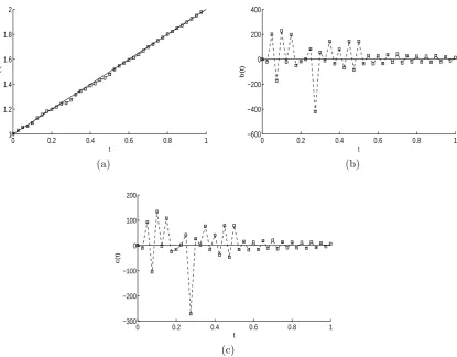
Next, in order to investigate the stability of the numerical solution we add some small percentage p = 0.1% of noise to the input data (11) and (12), as in (78) for k = 1,2. We have also investigated higher amounts of noisep, but the results obtained were less accurate hence, they are not presented. However, similar qualitative conclusions, regarding achiev-ing stability through regularization, maintain. Details regardachiev-ing the number of iterations, number of function evaluations, value of the objective function (75) at the final iteration, the rmsevalues (80)–(82) and the computational time taken for running the iterative mini-mization routinelsqnonlin are summarised in Table 1. One can notice that it takes almost one day to run the program without regularization.

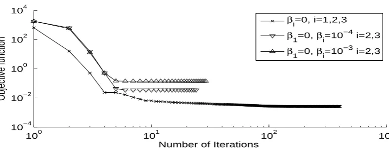
The objective function (75), as a function of the number of iterations, is plotted in Figure 3. From this figure it can be seen that in the absence of regularization, see the graph for βi = 0, i = 1,2,3, a slow convergence is recorded and, in fact, the process of minimization

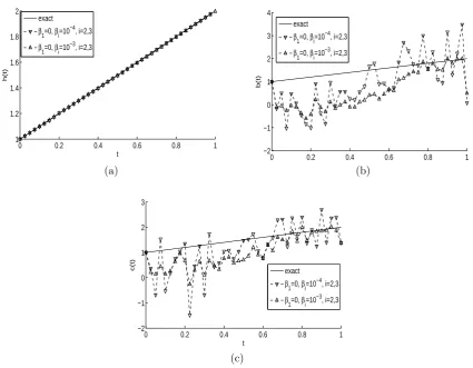
the stability of the solution in the components b(t) and c(t). Since in Figure 4(a) the free boundary has been obtained accurately, we fixβ1 = 0 and we only takeβ2 andβ3 as positive

regularization parameters in (75). These regularization parameters have been chosen by trial and error, and some numerical results obtained from a couple of choices are given in Table 1, and Figures 3 and 5. Justifying more rigorously the choice of multiple regularization parameters in the nonlinear Tikhonov regularization method is very challenging and will be the object of future numerical investigations. At this stage, we only mention the idea of extending to the nonlinear case some possible strategies of multi-parameter selection for the linear Tikhonov regularization suggested in [3]. From Figure 3 it can be noticed that a rapid convergence in less than 30 iterations is achieved for each selection of regularization parameters. Furthermore, from Table 1 it can be seen that the computational time is reduced from 1 day to less than an hour by the inclusion of regularization in (75).

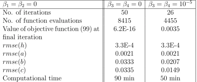
Table 1: Number of iterations, number of function evaluations, value of the objective function

(75) at final iteration, rmse values (80)-(82) and the computational time, for p = 0.1% noise for

Example 1.

β1 = 0 β2 =β3 = 0 β2 =β3 = 10−4 β2 =β3 = 10−3

No. of iterations 401 23 28

No. of function evaluations 49446 2976 3596

Value of objective function (75) at final iteration

0.0026 0.0345 0.1412

rmse(h) 0.0108 0.0026 0.0040

rmse(b) 105.34 1.1044 1.0787

rmse(c) 61.838 0.8184 0.6558

Computational time 23 hours 40 min 45 min

100 101 102 103

10−4 10−2 100 102 104

Number of Iterations

Objective function

β_i=0, i=1,2,3

β₁=0, β

i=10

−4

i=2,3

β₁=0, β

i=10

−3

i=2,3

Figure 3: The objective function (75) for p= 0.1% noise for Example 1.

0 0.2 0.4 0.6 0.8 1 1

1.2 1.4 1.6 1.8 2

t

h(t)

(a)

0 0.2 0.4 0.6 0.8 1

−600 −400 −200 0 200 400

t

b(t)

(b)

0 0.2 0.4 0.6 0.8 1

−300 −200 −100 0 100 200

t

c(t)

(c)

Figure 4: The exact (—) and numerical (_{−−) solutions for: (a) the free boundary h(t), (b) the}

coefficientb(t), and (c) the coefficient c(t), withp= 0.1% noise and no regularization for Example

1.

5.2

Example 2

We consider now the second inverse problem (1)–(3), (5), (6) and (34) with unknown coeffi-cientsh(t), b(t) and c(t), with the same input data as in Example 1 of Subsection 5.1, but in which the Stefan condition dataµ3(t) given by equation (4) is replaced by the third-order

heat momentµ6(t) given by equation (35) as

µ6(t) =

e3t 2 (t

2

−1 + 2 ln(2 +t)), t _∈[0,1].

One can remark that conditions of Theorem 2 are satisfied and therefore, the local existence of a unique solution is guaranteed. Furthermore, one can observe that the function (54) given by

D2(t) =−(1/2)e6t

(

(t₋1)(1 +t)2+ (7 + 10t+ 3t2) ln(2 +t)

−2(2 +t)2ln2(2 +t)

)

, t _∈[0,1], (89)

solution is the same as that given by equations (84) and (85). All the computational details are the same as for Example 1.

0 0.2 0.4 0.6 0.8 1

1 1.2 1.4 1.6 1.8 2

t

h(t)

exact

β₁=0, β

i=10 −4

, i=2,3

β 1=0, βi=10

−3

, i=2,3

(a)

0 0.2 0.4 0.6 0.8 1

−2 −1 0 1 2 3 4

b(t)

exact

β₁=0, β

i=10 −4_{, i=2,3}

β₁=0, β

i=10 −3

, i=2,3

(b)

0 0.2 0.4 0.6 0.8 1

−2 −1 0 1 2 3

t

c(t) _exact

β 1=0, βi=10

−4

, i=2,3

β 1=0, βi=10

−3_{, i=2,3}

(c)

Figure 5: The exact and numerical solutions for: (a) the free boundary h(t), (b) the coefficient b(t), and (c) the coefficientc(t), with p= 0.1% noise and regularization for Example 1.

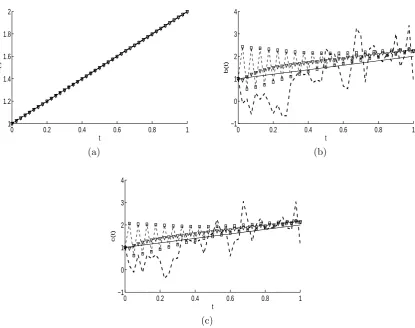
As we did in Example 1, we start with the case of exact input data (11), (12) and (35), i.e. p = 0 in (79). The objective function (76), as a function of the number of iterations is displayed in Figure 6. From this figure it can be noticed that a monotonic convergence is rapidly achieved (in the early few iterations) and then turn to a steady slow convergence. The objective function (76) decreases and takes stationary values ofO(10−11_{) andO(10}−6_{) in} about 401 and 112 iterations forβi = 0, i= 1,2,3, andβ1 = 0, β2 =β3 = 10−8, respectively.

The numerical results for the unknown coefficients are illustrated in Figure 7. From this figure it can be noticed that, as in Example 1, a stable and very accurate recovery for the free boundary h(t) is obtained with a small rmse(h) = 0.001. With no regularization, the numerical results for b(t) and c(t) are quite unstable and inaccurate with rmse values of 0.5962 and 0.4279, respectively. However, when we apply the regularization with β1 = 0,

and β2 =β3 = 10−8 to (76) we obtain more stable and accurate reconstructions for b(t) and

c(t) with rmse values decreasing to 0.2908 and 0.1838, respectively.

Next, we consider the case of noisy input data (11), (12) and (35) and perturb them with p = 0.01% as in (78). Remark that in Example 2 we include noise in all the input data µ4, µ5 and µ6, whilst in Example 1 noise was included only in µ4 and µ5. Therefore,

with that of Example 1, indicates that the second inverse problem (1)–(3), (5), (6) and (34) is more ill-posed than the first inverse problem (1)–(6). The case when no regularization is included, i.e. βi = 0 for i= 1,2,3, is omitted since a similar unstable behaviour to Example

1 shown in Figures 4(b) and 4(c) was obtained. The regularized objective function (76) with β1 = 0, β2 = β3 = 10−6 shown in Figure 6 decreases rapidly and takes a stationary value

of O(10−3_{) in 63 iterations. With this selection of regularization parameters, the unknown}

coefficients are plotted in Figure 7 using the dashed line style (- - -). The coefficients are reconstructed with reasonable accuracy having thermsevalues of 0.0022, 0.9498 and 0.6781 forh(t),b(t) and c(t), respectively.

100 101 102 103

10−15

10−10

10−5

100

105

Number of Iterations

Objective function

Figure 6: The objective function (76) with no regularization (-_×-) and with regularization

param-etersβ1 = 0,β2 =β3 = 10−8 (-△-), without noise for Example 2. We also include with (--) the

results forp= 0.01% noise, with regularization parameters β1 = 0, β2=β3 = 10−6.

The next section investigates inverse problems similar to those of Sections 2, 4 and 5, but in which the time-dependent thermal conductivity is an additional unknown.

6

Triple coefficient extension

Consider the one-dimensional time-dependent heat equation

∂u

∂t(x, t) =a(t) ∂2_u

∂x2(x, t) +b(t)

∂u

∂x(x, t) +c(t)u(x, t) +f(x, t), (x, t)∈Ω (90)

for the unknown temperature u(x, t) with unknown free smooth boundary x = h(t) > 0 and time-dependent coefficients a(t) >0, b(t) and c(t). The initial and Dirichlet boundary conditions are (2) and (3), respectively, and the over-determination conditions are (4)–(6), together with the heat flux specification atx= 0, namely,

0 0.2 0.4 0.6 0.8 1 1

1.2 1.4 1.6 1.8 2

t

h(t)

(a)

0 0.2 0.4 0.6 0.8 1

−1 0 1 2 3 4

t

b(t)

(b)

0 0.2 0.4 0.6 0.8 1

−1 0 1 2 3 4

t

c(t)

(c)

Figure 7: The exact (—) and numerical solutions with no regularization (_{), and with}

regular-ization parametersβ1 = 0, β2 =β3 = 10−8 (△△△) without noise for Example 2. We also include

with (- - -) the numerical results for p = 0.01% noise with regularization parameters β1 = 0,

β2=β3 = 10−6 for: (a) the free boundaryh(t), (b) the coefficientb(t), and (c) the coefficient c(t).

As in Section 2, by performing the change of variable y=x/h(t) we reduce the problem (2)–(6), (90) and (91) to the inverse problem for the unknowns h(t), a(t), b(t), c(t) and v(y, t) :=u(yh(t), t) given by:

∂v

∂t(y, t) = a(t) h2_(t)

∂2_v

∂y2(y, t) +

b(t) +yh′_(t) h(t)

∂v

∂y(y, t) +c(t)v(y, t)+f(yh(t), t),

(y, t)_∈QT, (92)

equations (8)–(12) and

−a(t)vy(0, t)

h(t) =˜µ3(t), t∈[0, T]. (93)

A slightly corrected version of the theorem proved in [19] ensures the unique solvability (locally in time) for the inverse problem (8)–(12), (92) and (93).

Theorem 3. Suppose that:

0 _≤ f _∈ C1,0_{([0,∞)×[0, T]), 0 < µ}

i ∈ C1[0, T] for i = 1,2,4,5, µ3 ∈ C[0, T], 0 > µ˜3 ∈

C[0, T], 0< ϕ_∈C2_{[0, h}

0], ϕ′ >0,

the compatibility conditions of the zero order:

ϕ(0) =µ1(0), ϕ(h0) =µ2(0),

∫h0

0 ϕ(x)dx=µ4(0),

∫h0

0 xϕ(x)dx=µ5(0), and of the first-order:

µ′

1(0) =a(0)ϕ′′(0) +b(0)ϕ′(0) +c(0)ϕ(0) +f(0,0),

µ′

2(0) =a(0)ϕ′′(h0) +b(0)ϕ′(h0) +c(0)ϕ(h0) +f(h0,0),

}

(95)

are satisfied. Then, there is T0 ∈ (0, T], such that there exists a unique solution (h(t),

a(t), b(t), c(t), v(y, t))_∈C1_{[0, T}

0]×(C[0, T0])3×C2,1(QT0), h(t)>0, a(t)>0 for t∈[0, T0], of the inverse problem (8)–(12), (92) and (93).

Remark. We can obtain the values of a(0), b(0) and c(0) directly from equations (93) and

(95). First, from (93) applied at t= 0 we have

a(0) =₋µ˜3(0)

ϕ′₍₀₎. (96)

Then, introducing (96) into (95) and solving the resulting system of equations for b(0) and c(0) we obtain

b(0) = ϕ(h0)

(

µ′

1(0) + ˜

µ3(0)ϕ′′(0)

ϕ′₍₀₎ −f(0,0)

)

−ϕ(0)(µ′

2(0) + ˜

µ3(0)ϕ′′(h0)

ϕ′₍₀₎ −f(h0,0)

)

ϕ(0)ϕ(h0)

(

ϕ′₍₀₎

ϕ(0) − ϕ′_(h0)

ϕ(h0)

) , (97)

c(0) =

ϕ′₍₀₎(_µ′

2(0) + ˜

µ3(0)ϕ′′(h0)

ϕ′₍₀₎ −f(h0,0)

)

−ϕ′_(h

0)

(

µ′

1(0) + ˜

µ3(0)ϕ′′(0)

ϕ′₍₀₎ −f(0,0)

)

ϕ(0)ϕ(h0)

(

ϕ′₍₀₎

ϕ(0) − ϕ′_(h0)

ϕ(h0)

) . (98)

One can easily remark that the conditions on ϕ given in Theorem 3 ensure that expressions (97) and (98) are well-defined. In particular, condition (94) implies that the function ϕ′_/ϕ is strictly monotone.

6.1

Another related inverse problem formulation

It was point out in [12] that the Stefan condition (4), or (10), may be replaced by the second-order moment measurement (34), or (35), respectively. Then we have the following local existence and uniqueness theorem, see [12] with appropriate corrections.

Theorem 4. Let the assumptions of Theorem 3 be satisfied, except for the condition on µ3

being replaced by the condition 0 < µ6 ∈ C1[0, T]. Then, there exists T0 ∈ (0, T], such that there exists a unique solution(h(t), a(t), b(t), c(t), v(y, t))_∈C1_{[0, T}

0]×(C[0, T0])3×C2,1(QT0),

h(t)>0, a(t)>0 for t_∈[0, T0], of the inverse problem (8), (9), (11), (12), (92) and (93).

6.2

Numerical implementation, results and discussion

inverse problems under investigation in Section 6 we minimize the functionals

˜

F(h, a, b, c) =

N

∑

j=1

[a_jv_y(0, t_j)

hj

+ ˜µ3(tj)

]2 + N ∑ j=1 [ h′ j +

vy(1, tj)

hj −

µ3(tj)

]2 + N ∑ j=1 [ hj ∫ 1 0

v(y, tj)dy−µ4(tj)

]2 + N ∑ j=1 [

h2_j

∫ 1

0

y2v(y, tj)dy−µ5(tj)

]2

+β1 N

∑

j=1

h2 j +β2

N

∑

j=1

a2 j +β3

N

∑

j=1

b2 j +β4

N

∑

j=1

c2

j, (99)

and

˜

F1(h, a, b, c) = N

∑

j=1

[a_jv_y(0, t_j)

hj

+ ˜µ3(tj)

]2 + + N ∑ j=1 [ hj ∫ 1 0

v(y, tj)dy−µ4(tj)

]2 + N ∑ j=1 [

h2_j

∫ 1

0

yv(y, tj)dy−µ5(tj)

]2 + N ∑ j=1 [

h3_j

∫ 1

0

y2v(y, tj)dy−µ6(tj)

]2

+β1 N

∑

j=1

h2_j +β2 N

∑

j=1

a2_j +β3 N

∑

j=1

b2_j +β4 N

∑

j=1

c2_j. (100)

The minimization of ˜F and ˜F1 subject to the physical constraints h >0 and a >0 are

pre-formed using the MATLAB optimization toolbox routinelsqnonlin, as described in Section 4. We also add noise in the heat flux (93), as described at the end of Section 4.

6.2.1 Example 3

We consider first the inverse problem (2)–(6), (90) and (91) with unknown coefficientsh(t), a(t), b(t) and c(t), and solve this problem with the following input data:

ϕ(x) =u(x,0) = (1 +x)2, µ1(t) =u(0, t) = 1 +t, µ2(t) =u(h(t), t) = (1 +t)(2 +t)2,

˜

µ3(t) =−a(t)ux(0, t) =−2(1 +t)2, µ3(t) = h′(t) +ux(h(t), t) = 1 + 2(1 +t)(2 +t),

µ4(t) =

∫ h(t)

0

u(x, t)dx= 1

3(1 +t)

2_{(7 + 5t+t}2_),

µ5(t) =

∫ h(t)

0

xu(x, t)dx= 1

12(1 +t)

3_{(17 + 14t+ 3t}2₎

f(x, t) = 2 + 5t+ 4t2_{+ 6x+ 12tx+ 8t}2_{x+ 2x}2_{+ 3tx}2_{+ 2t}2_x2_{, h}

0 = 1, T = 1.

One can remark that the conditions of Theorem 3 are satisfied and hence, the local unique solvability of the inverse problem holds. With the data above, the analytical solution is given by

h(t) = 1 +t, a(t) = 1 +t, b(t) = ₋1₋2t, c(t) =₋1₋2t, (101)

u(x, t) = (1 +t)(1 +x)2. (102)

Then, (101) and

is the analytical solution of the problem (8)–(12), (92) and (93).

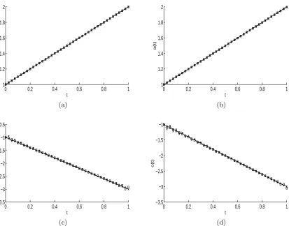
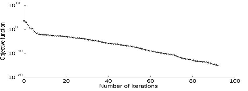
The initial guess for the vectorsh,a, b and care taken as 1, 1, ₋1 and ₋1, respectively. We start the numerical discussion with the case of exact data, i.e. p = 0 in (79). The objective function (99), as a function of the number of iterations, is shown in Figure 8. From this figure it can be seen that a monotonic convergence is achieved in 50 iterations if no regularization is applied. The unregularized objective function (99) decreases rapidly in the first 10 iterations and then steadily reaches a stationary low value of O(10−16_{). The}

numerical results for the unknowns coefficients h(t), c(t), b(t) and c(t) are represented in Figures 9(a)–(d) by the (₋x₋) lines. From these figures it can be observed that we obtain accurate and stable reconstructions for free boundaryh(t) and the thermal conductivitya(t), whilst for the coefficients b(t) and c(t) some very slight instabilities appear. Consequently, we do not need to regularize h(t) and a(t) and therefore, we are take β1 = β2 = 0 in (99)

and apply the Tikhonov regularization method with some small regularization parameters β3 =β4 = 10−5. The accurate and stable numerically obtained results are shown in Figures

9(a)–(d) by the (-_{-) line. The regularized objective function (99) for this case is also plotted}

in Figure 8 and a rapid monotone convergence is obtained in 26 iterations. A summary of all details is presented in Table 2, where thermse(a) is defined, similarly as in (80)–(82), as

rmse(a) =

v u u t

T N

N

∑

j=1

(anumerical(tj)−aexact(tj))2. (104)

Table 2: Number of iterations, number of function evaluations, value of the objective function (99)

at final iteration, rmse values (80)-(82) and (104), and the computational time, without noise for

Example 3.

β1 =β2 = 0 β3 =β4 = 0 β3 =β4 = 10−5

No. of iterations 50 26

No. of function evaluations 8415 4455

Value of objective function (99) at final iteration

6.2E-16 0.0035

rmse(h) 3.3E-4 3.3E-4

rmse(a) 0.0021 0.0021

rmse(b) 0.0333 0.0207

rmse(c) 0.0335 0.0149

0 10 20 30 40 50 10−20

10−10 100 1010

Number of Iterations

Objective function

β_i=0, i=1,2,3,4

β_i=β

2=0, βi=10

−5_{, i=3,4}

Figure 8: The objective function (99) without noise for Example 3.

0 0.2 0.4 0.6 0.8 1

1 1.2 1.4 1.6 1.8 2

t

h(t)

(a)

0 0.2 0.4 0.6 0.8 1

1 1.2 1.4 1.6 1.8 2

t

a(t)

(b)

0 0.2 0.4 0.6 0.8 1

−3.5 −3 −2.5 −2 −1.5 −1 −0.5

t

b(t)

(c)

0 0.2 0.4 0.6 0.8 1

−3.5 −3 −2.5 −2 −1.5 −1

t

c(t)

(d)

Figure 9: The exact (—) and numerical solutions (₋x₋) without regularization, and (_{−−) with}

regularization parametersβ1 =β2 = 0, andβ3 =β4 = 10−5 for: (a) the free boundaryh(t), (b) the

coefficienta(t), (c) the coefficientb(t), and (d) the coefficientc(t), without noise for Example 3.

Next, we investigate the stability of the numerical solution with respect to some small percentagep= 0.1% of noise included in the input data ˜µ3(t),µ4(t) andµ5(t). The objective

tolerance is reached. On the other hand, the numerical solutions for the unknown coefficients plotted in Figure 11 are oscillatory and highly unstable except for the free boundary h(t) which is accurate and stable. There is also some slight instability manifested in Figure 11(b) in estimating the coefficient a(t), but the magnitude of these oscillations is significantly much smaller than the highly unbounded and unstable behaviour shown in Figures 11(c) and 11(d) illustrating the estimation of the unregularized coefficients b(t) and c(t), respectively. As a result, we can take β1 = β2 = 0 and then minimize (99) with various regularization

parameters β3 = β4 ∈ {10−4,10−3,10−2}. Figure 12 shows the rapid monotonic decreasing

convergence of the regularized objective function, as the number of iterations increases. The corresponding numerical results for the unknown time-dependent coefficients are shown in Figures 13. A summary of the computational details, as well as thermseerrors are included in Table 3. Overall, by comparing Figures 11 and 13 it can be observed some remarkable stability restored through the inclusion of regularization. It is also interesting to remark that although we takeβ2 = 0 and hence we do not penalise the coefficienta(t) in (99), some

of the regularization of the other two coefficients b(t) and c(t) is transferred to the former unregularized coefficient a(t), compare Figures 11(b) and 13(b).

0 20 40 60 80 100

10−20 10−10 100 1010

Number of Iterations

Objective function

Figure 10: The objective function (99) withp= 0.1% noise and no regularization for Example 3.

Table 3: Number of iterations, number of function evaluations, value of the objective function (99)

at final iteration,rmsevalues (80)-(82) and (104), and the computational time, forp= 0.1% noise

for Example 3.

β1 =β2 = 0 β3 =β4 = 0 β3=β4=10−4 β3=β4=10−3 β3=β4=10−2

No. of iterations 92 27 25 30

No. of function evaluations 15354 4620 4290 5115

Value of objective function (99) at final iteration

8.4E-16 0.0449 0.3660 3.5102

rmse(h) 0.0043 0.0026 0.0022 0.0032

rmse(a) 0.2508 0.0487 0.0253 0.0398

rmse(b) 8.3489 0.5420 0.1991 0.2276

rmse(c) 7.8212 0.4354 0.1563 0.1646

0 0.2 0.4 0.6 0.8 1 1

1.2 1.4 1.6 1.8 2

t

h(t)

(a)

0 0.2 0.4 0.6 0.8 1

0 0.5 1 1.5 2 2.5

t

a(t)

(b)

0 0.2 0.4 0.6 0.8 1

−30 −20 −10 0 10 20

t

b(t)

(c)

0 0.2 0.4 0.6 0.8 1

−20 −10 0 10 20

t

c(t)

(d)

Figure 11: The exact (—) and numerical solution (_{−−) for: (a) the free boundaryh(t), (b) the}

coefficient a(t), (c) the coefficient b(t), and (d) the coefficient c(t), with p = 0.1% noise and no

regularization for Example 3.

0 5 10 15 20 25 30

10−2 100 102 104

Number of Iterations

Regularized objective function