Rochester Institute of Technology
RIT Scholar Works
Theses Thesis/Dissertation Collections
8-2014
Tiered Based Addressing in Internetwork Routing
Protocols for the Future Internet
Yoshihiro Nozaki
Follow this and additional works at:http://scholarworks.rit.edu/theses
This Dissertation is brought to you for free and open access by the Thesis/Dissertation Collections at RIT Scholar Works. It has been accepted for inclusion in Theses by an authorized administrator of RIT Scholar Works. For more information, please [email protected].
Recommended Citation
Tiered Based Addressing in
Internetwork Routing Protocols
for the Future Internet
by
Yoshihiro Nozaki
A Dissertation Submitted in Partial Fulfillment of the Requirements for the Degree of Doctorate of Philosopy in
Computing and Information Sciences
B.Thomas Golisano College of Computing and Information Sceince
Department of Computing and Information Science
Rochester Institute of Technology Rochester, NY
B. Thomas Golisano College of Computing and Information Sciences Rochester Institute of Technology
Rochester, New York
Certificate of Approval
Ph.D. Degree
The Ph.D. Degree of Yoshihiro Nozaki
has been examined and approved by the dissertation committee as satisfactory for the dissertation required for the
Ph.D. degree in Computing and Information Sciences
Approved by:
Committee Approval:
Dr. Nirmala Shenoy, Dissertation Advisor
Dr. Aparna Gupta, Dissertation Committee Member
Dr. Tae Oh, Dissertation Committee Member
Dr. Kaiqi Xiong, Dissertation Committee Member
c
Abstract
The current Internet has exhibited a remarkable sustenance to evolution and growth; however, it is facing unprecedented challenges and may not be able to continue to sustain this evolution and growth in the future because it is based on design decisions made in the 1970s when the TCP/IP concepts were developed. The research thus has provided incremental solutions to the evolving Internet to address every new vulnerabilities. As a result, the Internet has increased in complexity, which makes it hard to manage, more vulnera-ble to emerging threats, and more fragile in the face of new requirements. With a goal towards overcoming this situation, a clean-slate future Internet architecture design paradigm has been suggested by the research communities. This research is focused on addressing and routing for a clean-slate future Internet architecture, called the Floating Cloud Tiered (FCT) internetworking model. The major goals of this study are: (i) to address the two related problems of routing scalability and addressing, through an approach which would leverage the existing structures in the current Internet architecture, (ii) to propose a solution that is acceptable to the ISP community that supports the Internet, and lastly (iii) to provide a transition platform and mechanism which is very essential to the successful deployment of the proposed design.
Bibliographic Notes
Most of the work presented in this thesis appears in previously published jour-nals and conference proceedings. The list of related publications are presented hereafter:
• Y. Nozaki, H. Tuncer, and N. Shenoy, ”A Tiered Addressing scheme based on a Floating Cloud Internetworking model,” in Proceedings of the 12th international conference on Distributed computing and networking, ICDCN’11, (Berlin, Heidelberg), pp. 382-393, Springer-Verlag, 2011.
• Y. Nozaki, H. Tuncer, and N. Shenoy, ”ISP tiered model based archi-tecture for routing scalability,” In Communications (ICC), 2012 IEEE International Conference on, pp. 5817-5821. IEEE, 2012.
• Y. Nozaki, P. Bakshi, and N. Shenoy, ”Tiered Interior Gateway Rout-ing Protocol,” In ICNS 2013, The Ninth International Conference on Networking and Services, pp. 68-75. 2013.
• Y. Nozaki, P. Bakshi, and N. Shenoy, ”A Novel Approach to Interior Gateway Routing,” International Journal On Advances in Networks and Services 6, no. 3 and 4 (2013): 208-219.
• Y. Nozaki, P. Bakshi, H. Tuncer, and Nirmala Shenoy. ”Evaluation of tiered routing protocol in floating cloud tiered internet architecture,” Computer Networks 63 (2014): 33-47.
• H. Tuncer, Y. Nozaki, and N. Shenoy, ”Virtual mobility domains − A mobility architecture for the future Internet,” In Communications (ICC), 2012 IEEE International Conference on, pp. 2774-2779. IEEE, 2012.
Acknowledgements
I am most grateful to my dissertation advisor, Dr. Nirmala Shenoy, who expertly guided me through the time of my dissertation research. Her enthusi-asm, encouragement, and faith in me throughout have been extremely helpful. She was always positive and gave generously of her time and vast knowledge. Without her guidance and persistent help this dissertation would not have been possible.
My application also extends to my committee members, Dr. Aparna Gupta, Dr. Tom Oh, and Dr. Kaiqi Xiong for serving as my committee mem-bers even at hardship. I would especially like to thank Dr. Aparna Gupta for her detailed comments and her recommendations regarding the economical study.
I would also like to thank all my colleagues, Hasan Tuncer and Yamin Al-Mousa, who shared research experiences with me from the beginning of the Ph.D. program, and Josh Watts, Alan Meekins, Arnav Ghosh, and Parth Bakshi, who contribute to the development of the FCT router in the testbed at RIT, and also to the movement of the software router to Emulab testbed.
Contents
Abstract . . . v
Bibliographic Notes . . . vii
Acknowledgements . . . ix
List of Tables . . . xiv
List of Figures . . . xvi
1 Introduction 1 2 Literature Review 7 2.1 Research Initiatives for the Future Internet Architecture . . . 7
2.1.1 Solutions Under the Current Internet Architecture . . . 8
2.1.2 Solutions Towards a Clean Slate Future Internet . . . . 9
2.2 Addressing in the Internet . . . 10
2.2.1 IP Address . . . 11
2.3 Routing in the Internet . . . 12
2.3.1 Intra Domain Routing . . . 13
2.3.2 Inter Domain Routing . . . 16
2.4 Adoption of New Network Architecture . . . 20
4 Methodology 24
4.1 ISP Tiered Structure . . . 24
4.1.1 Tiered Structure within an ISP . . . 26
4.1.2 Tiered Structure among ISPs . . . 28
4.1.3 Nesting, Decoupling, and Floating Properties . . . 30
4.2 Tiered Routing Address (TRA) . . . 31
4.2.1 Nested TRA . . . 33
4.2.2 TRA Address Format . . . 35
4.3 Tiered Routing Protocol (TRP) . . . 36
4.3.1 TRA Allocation Process . . . 36
4.3.2 Populating Routing Tables . . . 37
4.3.3 Packet Forwarding . . . 39
4.3.4 Failure Detection and Handling . . . 41
4.4 Integration of Inter and Intra Domain Routing . . . 45
4.4.1 MMT Routing in a Cloud . . . 46
4.5 TRP Code and Local Testbed . . . 49
5 Evaluation of TRA and TRP 51 5.1 Evaluation of TRP in Intra-domain Routing . . . 51
5.1.1 Analyzing AT&T Network . . . 52
5.1.2 Tiered Structure and TRA allocation . . . 57
5.1.3 Address Length and Numbers . . . 59
5.1.4 HD Ratio for Address Allocation Efficiency . . . 63
5.1.5 Routing Table Size Analysis of TRP . . . 67
5.2 Evaluation of TRP in Inter-domain Routing . . . 82
5.2.1 Analyzing Worldwide AS Network . . . 82
5.2.2 AS Tiers and TRA Allocation . . . 84
5.2.3 Churn Rate Analysis of TRP . . . 90
5.2.4 Routing Table Size Analysis of TRP . . . 92
5.2.5 Performance Statistics and Analysis of TRP on Testbed 94 5.3 Evaluation of Integrated TRP and MMT . . . 97
5.3.1 IP+OSPF . . . 97
5.3.2 TRP+MMT . . . 99
5.3.3 Results . . . 99
5.4 Transition Study with MPLS Approach . . . 100
5.5 Discussions . . . 105
6 Transition Study with Economic Model 107 6.1 Assumptions and Cost Entities . . . 108
6.1.1 Transition Model . . . 108
6.2 Types and Number of Routers . . . 110
6.2.1 Identification of Router Types by Connectivity . . . 111
6.3 Modeling . . . 111
6.3.1 Router Investment Cost (IC) and Salvage Value . . . . 112
6.3.2 Router Maintenance Cost (RM) . . . 114
6.3.3 Human Resource Cost (HR) . . . 115
6.3.4 Power Usage Cost (PU) . . . 117
6.3.5 Total Running Costs and Transition Scenarios . . . 119
6.4 Complexity of Routing Protocol . . . 120
6.4.2 Method of Populating Routing Table . . . 122
6.5 Transition Scenarios and Estimation . . . 123
6.5.1 Number of Each Router Type . . . 123
6.5.2 Router Investment Cost and Salvage Value . . . 124
6.5.3 Router Maintenance Cost . . . 125
6.5.4 Human Resource Cost . . . 125
6.5.5 Power Usage Cost . . . 127
6.5.6 Operating Cost Estimation . . . 129
6.5.7 Transition Cost Estimation . . . 137
6.6 Limitations . . . 143
7 Conclusion 144 A Internet Topology 148 A.1 POP Level Topology of ISPs . . . 148
A.2 Router Level Topology of AT&T . . . 149
B Multi-Meshed Tree (MMT) 152
C Router Statistics of AT&T 155
List of Tables
4.1 Routing Tables of Router F . . . 38
4.2 Routing Tables of Router G . . . 38
5.1 Number of Routers at each POP in AT&T . . . 55
5.2 AT&T Network Statistics based on TRA . . . 62
5.3 Number of Nodes in each Tier Level . . . 65
5.4 IP Routing Table of Router B in Figure 5.15 . . . 67
5.5 Emulab Testbed Configurations . . . 72
5.6 List of Tier 1 Provider ASs . . . 85
5.7 Largest Address Tree at Each Tier(Largest base) . . . 89
5.8 Largest Address Tree at Each Tier(Smallest base) . . . 90
5.9 LER MPLS Table of Router A{3.1:1:1} . . . 101
5.10 LER MPLS Table of Router F {3.1:3:1} . . . 101
5.11 LSR MPLS Table of Router B {2.1:1} . . . 102
5.12 LSR MPLS Table of Router C {1.1} . . . 102
5.13 LSR MPLS Table of Router D {2.1:3} . . . 103
6.1 Annual Energy Consumption and Costs of ISPs . . . 117
6.2 Route Maintenance Complexity of OSPF and TRP . . . 122
6.4 Price of Router Maintenance Service . . . 125
6.5 Salary of Network Administrator in the US . . . 126
6.6 Employment Ratio of Occupations . . . 126
6.7 Estimated Network Administrators in AT&T . . . 127
6.8 Power Consumption of Router Types . . . 128
6.9 Breakdown of Power Consumption by a Router . . . 128
6.10 Ratio of Costs (AR based) . . . 130
6.11 Total Number of Routers before and after Transition . . . 130
List of Figures
4.1 Typical ISP Tier Structure . . . 25
4.2 AT&T POP Level Network in the US . . . 26
4.3 NY-POP Router-level network in AT&T . . . 27
4.4 Business Relationships between ISPs . . . 28
4.5 Worldwide Internet AS tiers . . . 29
4.6 Tiered Topology and Tiered Routing Address . . . 31
4.7 Example of Nested TRAs . . . 34
4.8 Address Format in FCT Packet . . . 36
4.9 TRA Allocation Process . . . 36
4.10 Failure Handling with Up-link . . . 42
4.11 Failure Handling with Down-link . . . 43
4.12 Trunk-link information sharing . . . 43
4.13 Address Changes in TRP . . . 44
4.14 Primary Address Change . . . 45
4.15 Example of MMT (Hop limit is 3) . . . 46
4.16 3-ways Handshake in MMT Joining Process . . . 47
4.17 Data Forwarding with MMT . . . 48
4.18 Local Testbed Topology . . . 50
5.1 US AT&T Network imported to OPNET . . . 52
5.2 AT&T Router-Level Network Topology . . . 53
5.3 AT&T NY Router-Level Topology . . . 53
5.4 AT&T SF Router-Level Topology . . . 54
5.5 AT&T Router Degree Distribution . . . 56
5.6 AT&T Router Shortest Path Length Distribution . . . 57
5.7 US AT&T POP Distribution . . . 58
5.8 BB Routers Distribution of AT&T Network . . . 59
5.9 Correlation between BB Routers and POP Size . . . 60
5.10 Original Seattle Topology of AT&T Network . . . 61
5.11 Seattle POP Topology of AT&T with FCT Model . . . 61
5.12 TRA Address Length Distribution across AT&T Network . . . 62
5.13 Total Size of TRA and IP Addresses . . . 63
5.14 Total Number of Allocated TRA and IP Addresses . . . 63
5.15 A Sample IP network Topology with 9 Subnets . . . 68
5.16 Routing Table Size of OSPF and TRP in AT&T . . . 70
5.17 Number of Updates of OSPF and TRP in AT&T . . . 71
5.18 Testbed Topology with Tiered Routing Addresses . . . 72
5.19 TRP Routing Convergence Time . . . 74
5.20 OSPF Routing Convergence Time . . . 75
5.21 TRP vs. OSPF Initial Convergence Time (sec) . . . 77
5.22 TRP vs. OSPF Routing Control Overhead Size (KB) . . . 78
5.23 TRP vs. OSPF Routing Table Entry Size . . . 78
5.24 TRP vs. OSPF Convergence Time after Failure (sec) . . . 79
5.25 TRP vs. OSPF Control Packet Size after Failure (KB) . . . . 80
5.27 Identified Worldwide AS Tiers . . . 84
5.28 Topology of Tier 1 ASs . . . 86
5.29 TRA Allocation to ASs . . . 87
5.30 Concept of TRA Address Tree . . . 88
5.31 Level3 Address Tree with and without Nesting . . . 88
5.32 Number of AS Impacted a Tier 1 AS (sorted) . . . 91
5.33 Average Number of Affected AS at Each Tier . . . 92
5.34 Routing Table Distribution of TRP . . . 93
5.35 Routing Table Size Distribution at Each Tier . . . 94
5.36 Testbed Topology used for BGP Comparison . . . 95
5.37 Maximum Routing Table Entry Size . . . 95
5.38 TRP vs. BGP Convergence Time after Failure . . . 96
5.39 AT&T Seattle POP for OSPF simulation . . . 98
5.40 MPLS Enabled Network with TRP . . . 100
6.1 Cost Components of Old/New Routing Protocols in an ISP . . 109
6.2 Distribution of BB, DR, and AR Routers (AT&T) . . . 131
6.3 Distribution of BB, DR, and AR after Transition(AT&T) . . . 132
6.4 Cost Ratio of RM (POP) . . . 133
6.5 Cost Ratio of HR (POP) . . . 134
6.6 Routing Table Ratio . . . 135
6.7 Complexity Ratio . . . 135
6.8 Cost Ratio of PU (POP) . . . 136
6.9 Transition Scenario in a POP . . . 138
6.10 Number of Each Router Types during Transition . . . 139
6.12 HR Cost ($) during Transition . . . 140
6.13 PU Cost ($) during Transition . . . 141
6.14 Total OC Cost ($) during Transition . . . 142
6.15 Investment Cost ($) during Transition . . . 142
6.16 Estimated Total Payout Period . . . 143
A.1 Level3 POP Level Topology in the US . . . 149
A.2 Sprint POP Level Topology in the US . . . 149
A.3 Router Level topology of AT&T . . . 150
A.4 Router Level topology of Chicago POP . . . 150
A.5 Router Level topology of Washington D.C. POP . . . 151
Chapter 1
Introduction
Japan, and the12th Five-Year Planprojects [6] by the Ministry of Science and Technology (MOST) in China. These programs support research efforts that target challenges such as routing, scalability, mobility, security, and reliability among others - towards an ideal future Internet architecture.
While designing future Internet architecture, an important consideration in the design of Internet architectures are testing and validation of the design and scalability using realistic network scenarios in a near realistic experimental setup. The Autonomous Systems (ASs) and Internet Service Providers (ISPs) that construct the current Internet would not be willing to expose their net-works to the risk of such experimentation, nor would they be willing to reveal information of their internal network topologies and implementations. Re-search communities have hence implemented open virtual large-scale testbeds using virtualization technologies. Large scale emulation and experimentation testbeds for this purpose are another effort sponsored and funded by major research organizations in the world; these include Global Environment for Net-work Innovations (GENI) [7] by NSF in the United States, the Future Internet Research and Experimentation (FIRE) project [8] a part of FP7 in the Euro-pean Union, the Japan Gigabit Network 2 Plus (JGN2plus) [9] and the China Next Generation Internet (CNGI) [10] testbeds in Asia. New architectures can be evaluated and improved by testing on these testbeds before finalizing and deploying the future Internet architecture in the real world.
Geff Huston [12] observed the growth of BGP (Border Gateway Protocol) routing table sizes for years and showed that one of the main contributions for the increasing the table size is due to an increasing number of multi-homed ASs. Because many of the ASs are moving from a single-homed connection to multi-homing and peering, the BGP table size has rapidly increased as the result of an increasingly dense interconnected AS mesh at the edge of the In-ternet. Furthermore, logical links achieved by Multiprotocol Label Switching (MPLS) technology have introduced meshed topologies within an ISP. The Level 3’s router topology presented in [13] is highly meshed because of this. Although flat and highly meshed network structures provide high redundancy, which comes at the cost of reduced efficiency as more and more complex routers are necessary to discover and maintain routes as the network grows in size, a fact that is apparently alarming when one notices the processing and opera-tional conditions of core routers today [14]. Routing loops, looping packets, and high network convergence times are also the costs attributed to meshed network structures. Scalability is difficult to achieve under these conditions. Meshed networks are also hard to upgrade, troubleshoot, and optimize unless they are designed using a simple and hierarchical model [11]. Unlike mesh net-works, the proposed tiered structure which optimally combines hierarchy and meshing provides a modular topology with good scalability. These advantages of tiered architectures let us recognize that it has the potential to address the issues that todays Internet has encountered.
as they still continue to exist, operationally, optimally combining hierarchy and meshing. With the modularity introduced through the concept of network clouds and nesting, the structure affords a high level of scalability [15]. The tier concept is common among ISPs, but it can also be noted within an ISP network which comprises several POPs, inside which three tiers can be identified; 1 comprises backbone routers, 2 comprises distribution routers, and tier-3 comprises access routers. In the proposed design, each set of routers is identified as a network cloud and then associated to a tier.
on suitably designed topologies. In addition to design and validate the FCT concept, cost estimation model for the transition is proposed.
Chapter 2
Literature Review
In this chapter, we briefly introduce research initiatives for the future Internet architecture. Next, the current Internet architecture and the main concept of intra-domain and inter-domain routing are briefly reviewed.
2.1
Research Initiatives for the Future
Inter-net Architecture
2.1.1
Solutions Under the Current Internet
Architec-ture
The Hierarchical Architecture for Internet Routing (HAIR) [17] targets lim-iting routing table size and decreasing churn rate by organized routing and applying a locator/identifier split approach in a hierarchical manner. The New Intern-Domain Routing Architecture (NIRA) adopts a provider-rooted hierar-chy and extends the hierarchical properties to addressing, to reduce both the number of forwarding entries and convergence times [18]. The Routing Archi-tecture for Next Generation Internet (RANGI) uses a locator/identifier split approach where a node’s ID is different from its locator address to provide routing scalability [19]. The Hybrid Link State Protocol (HLP) leverages the natural hierarchy of the AS structures in route aggregation to reduce route churning [20].
An Internet Engineering Task Force (IETF) research group proposes a core-edge separation, address indirection, and a map-and-encap approach towards reduced routing table sizes [21]. The Routing on Flat Labels (ROFL) proposes a naming architecture, and a routing architecture based on flat identifiers that has no location semantics for both inter and intra-domain routing [22]. The Enhanced Mobility and Multi-homing Supporting Identifier Locator Split Ar-chitecture (MILSA) proposes a hybrid design combining the locator/ID split and core-edge separation paradigms to provide renumbering, routing scalabil-ity, and mobility support among others [23].
the identity and location function of IP addresses remain the same while nodes are mobile [24]. The Internet Indirection Infrastructure (i3) Robust Overlay Architecture for Mobility (ROAM) provides a rendezvous based overlay indi-rection service that forwards data communication to the recent location of the mobile nodes efficiently [25].
2.1.2
Solutions Towards a Clean Slate Future Internet
Several clean slate future Internet projects were funded by NSF in the United States under its FIND program and subsequently under the FIA program. Some of these projects target routing scalability including the Floating Cloud Tiered Architecture [15] proposed by the authors. The eXpressive Internet Architecture (XIA) [26] aims to preserve the strengths of current Internet ar-chitecture while substantially improving security, and building in the ability to support evolving network functionality over time. XIA introduces a new protocol called XIP as a replacement for IP which introduces a new protocol stack, rich addressing and per-hop forwarding semantics [26]. The Mobility-First Project aims to address mobility, multihoming, connectivity robustness, context-aware routing and security by following key design principles such as separation of names from addresses, decentralized naming service, and a gen-eralized delay tolerant network (GDTN) with storage-aware routing [27].
scheme, Quality of Service (QoS) routing and resource Control (QoS-RRC). This mechanism is adopted to provide best network resources for reliable com-munication. Daidalos [29], another EU large-scale collaborative future Internet project, provides a virtual identity framework for a large number of users to access personalized services on seamlessly integrated heterogeneous network technologies with the help of an ID-Broker and an ID-Manager in a scalable manner.
The Japanese National Institute of Information and Communications Tech-nology supports AKARI: Architecture Design Project for New Generation Net-work [30]. AKARI applies an ID/locator split and a cross layer design approach to support more diverse services, mobility and multihoming to a larger number of users through dynamic heterogeneous environments and devices. AKARI keeps the ID-locator mapping at the edge of the network to respond to the mobility and multihoming of the node while keeping the global locator based routing system in the core of the network for scalability purposes. For transi-tion purposes they claim that the first 64 bits of the IPv6 address can be used as an ID and the remaining bits can be used as the locator.
2.2
Addressing in the Internet
uses an IP address as a location identifier. However, the process becomes diffi-cult because the IP address is a logical address that is allocated dynamically to a node and does not have any relationship with the actual location of the node. Further, the route itself is a path through the intricate mesh of networks that forms the Internet. If a network or a device fails, the connectivity information of thousands of networks and networked devices can be impacted causing very long network convergence delays and packet loss. Though robust due to redun-dant paths, the process of IP address allocation, combined with the high mesh connectivity has resulted in huge routing table sizes leading to routing scala-bility problems and its adverse impact on Internet performance such as high churn rates, high convergence times, and looping of packets amongst others.
2.2.1
IP Address
The original design of TCP/IP supported a maximum of 256 networks because it was believed that 256 networks would be sufficient [31]. IPv4 was then deployed to accommodate the growing number of networks through IP classes such as Class A, B, C, D, and E and eventually Network Address Translation (NAT) and Classless Inter-Domain Routing (CIDR) were introduced to cope with the growing demands. IPv6 was meanwhile developed to address the fast depletion of IPv4 addresses, to avoid address space fragmentation and to improve routing aggregation through hierarchical address allocation with a policy to avoid unnecessary and wasteful allocation [32].
a hierarchical manner to avoid fragmentation of address space and to better aggregate routing information. Meanwhile, the IPv6 policy tries to avoid un-necessary and wasteful allocation [32]. It is difficult to avoid fragmentation and wasteful address allocation at the same time because future address re-quirements from organizations and end sites are unpredictable and most times exhibit an exponential increase [32]. Therefore, when an additional address space is required, a sequential address space may not be available and frag-mentation of the address space is inevitable even with the huge IPv6 address pool.
2.3
Routing in the Internet
Internet Protocol (IP) provides best effort reachability for communication across networks and nodes connected to the Internet. In IP networks, routers use routing protocols to discover and maintain routes and also to recover from route failures. Routing tables maintained by current routing protocols increase almost linearly with increase in network size and is an unhealthy trend indi-cating scalability issues which can manifest as performance degradation. Also, the time taken for the network to adapt to topological changes increases with increase in network size resulting in higher convergence times during which routing is unpredictable and unstable. With more and more users connect-ing to networks today, this poses a serious problem. Patch and evolutionary solutions have been and are being proposed and implemented to address the problem both at the inter domain and intra domain level [33, 34].
and exterior gateway protocols (EGPs) respectively. Intra-domain routing provides connectivity with in single routing domain network of a company, an organization, or an ISP, often referred to Autonomous System (AS). Inter-domain routing provides connectivity between ASs.
2.3.1
Intra Domain Routing
Interior Gateway Protocols (IGP) such as Routing Information Protocol (RIP) and OSPF were designed to work with IP. RIP is a distance vector (DV) protocol and can be used in networks with a maximum diameter of 15 hops. Large ISP networks thus use Link-State (LS) IGPs such as IS-IS or OSPF which uses the area concept to segment networks into manageable size. LS routing protocols require periodic updates and redistribution of updates to all routers in the network or in an area on link state changes. Each router running the LS routing protocol executes the Dijkstras algorithm on the collected link state information to populate routing tables. Dissemination of network-wide (or area-wide) link state information also adversely impacts scalability and convergence times in the networks using OSPF. In some cases the physical location of areas requires use of virtual links to the backbone area further limiting the versatility of OSPF.
pro-tocol, overcame the scalability limitations by introducing areas, where within each area a separate copy of the basic link-state routing algorithm could be run. Each area thus had its own link-state database, and the topology was in-visible from outside of the area. This isolation enabled the protocol to reduce convergence times and the amount of routing traffic. Both routing protocols are IP based. RIP uses the distance vector approach, where routers record the next hop, towards other networks, and requires routers to advertise their rout-ing tables. OSPF runs Dijkstras algorithm on network topology information collected by nodes. Advertising routing tables and requiring network wide link state information adversely impact scalability and convergence.
Significant research effort has been directed towards the reduction and optimization in IGP convergence time to link status changes in the network. In this research area, the approaches can be categorized into two: reducing failure detection time and reducing routing information update time.
To reduce failure detection time, layer-2 notification is used to achieve sub-second link/node failure detection. However this relies on types of network interfaces and does not apply to switched Ethernet [35].
failure detection time, but at the expense of increased bandwidth usage due to increase in the number of periodic hello packets. Increased number of hello packets in a short interval can also increase possibility of route flaps.
Although link/node failure detection time can be reduced to sub-seconds, propagating the link status to all routers in the network takes time and is dependent on the network size.
To reduce such delays, an approach that suggests the use of several pre-computed back up routing paths was proposed. Pan et al. [36] proposed the MPLS based on a backup path to reroute around failures. However, having all possible MPLS back up paths in a network is not efficient. Multiple Routing Configurations (MRC) [37] uses a small set of backup routing paths to allow immediate packet forwarding on failure detection. A router in MRC maintains additional routing information on alternative paths. However, MRC guaran-tees recovery only from single failures. Liu at el. [38] proposed the use of pre-computed rerouting paths if the same can be resolved locally. Otherwise multi-hop rerouting path had to be set up by signaling to a minimal number of upstream routers. Another approach limits the propagation area of link state update after failure. Narvaez [39] proposed limited flooding to handle link failures. When a link failure occurs, the descendants of the failed link in the shortest path tree are determined and the new shortest path without the failed link is calculated. Then, the updated information is propagated in only the area of descendant nodes.
provide the opportunity to view the routing problem from a fresh perspective and thus design solutions that are not constrained by the current architectures or implementations.
2.3.2
Inter Domain Routing
The Internet is comprised of more than 73,700 Autonomous Systems (ASs) all over the world today [40] and inter-domain routing maintains routes between those ASs. This high load in the core routers is indicative of an imbalance in the routing information handling, which could adversely impact the advan-tages of the meshed structure, by making the routers a potential bottleneck. Furthermore, the constant increase in routing table sizes is likely to become unmanageable in the near future. The complexity of BGP is reflected in both the exterior BGP (eBGP) and interior BGP (iBGP) as they make complex decisions that combine technical route criteria with policies and service level agreements across networks belonging to different ASs.
In general, ASs have either a customer-provider or a peer-to-peer relation-ship with neighboring ASs. A customer pays its provider for transit and peers provide connectivity between their respective neighbor ASes. Based on the AS relationships, the tiered structure and the hierarchy in the AS topology becomes obvious when looking at the Internet [41].
the end-to-end AS paths. This reachability information is learned by BGP sessions which are exchanging information between BGP routers in different ASs. This is referred as external BGP (eBGP) session. On the other hand, internal BGP (iBGP) sessions are established within the same AS to share the reachability information obtained by eBGP. The reachability information is built by BGP advertisement. The advertisement contains the prefix of the destination network and the complete AS path to the destination network. The simplified operation of BGP can be categorized into four components.
The area of inter-domain routing protocol has been considered as one of significant challenging research topics in the Internet today. As the Internet has grown largely, routing table size of BGP core router, the number of ASes in the Internet, and the number of connections per AS to the network are also increased significantly [40, 43]. As the result, slow convergence and lack of scalability have been recognized as main issues by researchers in inter-domain routing area [33].
technology is more taxed. The current air cooling system is starting to be a limiting factor for scaling high-performance routers [14].
added location information of a root-cause into each BGP message when fail-ure occurs. With this failfail-ure location information, distant BGP routers can avoid to select alternate AS path which is also affected by the failure.
2.4
Adoption of New Network Architecture
Chapter 3
Research Questions
In the previous chapters, research challenges in both inter- and intra-domain routing protocols are presented in detail, both inter- and intra-domain routing are managed by those autonomous entities, which perform their own routing management based on policies that only have local significance. With this condition, new proposed solutions are difficult to implement or adopt in oper-ational networks because it is too heavyweight to be deployed and standard-ization work is not well advanced, especially for inter-domain routing because of its worldwide deployment. Therefore, transition from current routing pro-tocols to new routing protocol is not attractive to ISPs and ASs. Indeed, most of the existing proposals have never moved into a deployment stage. Thus, it is important to provide realistic and attractive scenario to the Internet service provider communities.
The questions that we intend to answer with our research are:
– Proposed new addressing scheme and routing protocol.
• The proposed solution is acceptable to the Internet service provider com-munities?
– Implemented software-based router and evaluated it in testbeds.
Chapter 4
Methodology
In this chapter, we first describe the existing tiered structure among the ISPs and within an ISP, and introduce new addressing and routing scheme used in the FCT Internet architecture.
4.1
ISP Tiered Structure
The Internet is comprised of more than 73,700 ASs today that operate the major flow of Internet communication and the current IP traffic represents in a way their business relationships. Any AS must pay for transit services to get Internet connectivity. In general, ASs have either a customer-provider or a peer-to-peer relationship with neighboring ASs. A customer pays its provider for transit and peers provide connectivity between their respective neighbor ASs. Based on the AS relationships, the tiered structure and the hierarchy in the AS topology becomes obvious when looking at the Internet.
Figure 4.1: Typical ISP Tier Structure
customers. The left part of Figure 4.1 visualizes the tiered structure described above and existing among ISPs today. In Figure 4.1, we show ISPs up to tier 3, and then show access networks connecting to the tier 3 ISPs.
4.1.1
Tiered Structure within an ISP
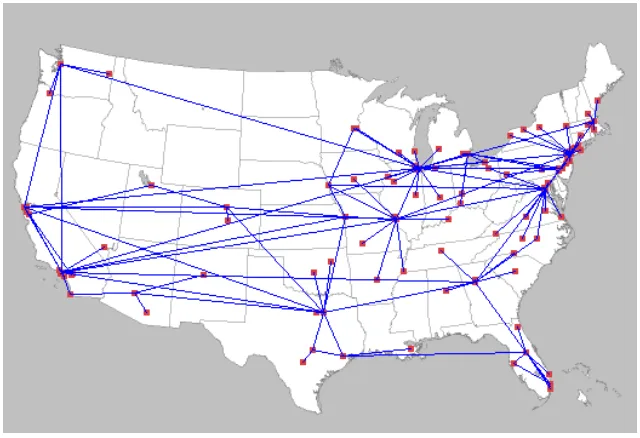
[image:46.612.146.466.298.517.2]To validate the tiered approach within an ISP, we used the Rocketfuel dataset [13]. This dataset has router-level connectivity information of ISPs. From the Rocketfuel dataset, we imported the AT&T router connectivity information using Cytoscape [62] that also helps to visualize AT&Ts router-level topology on the US map (this excludes Hawaii and Alaska). The dataset contains not only the connectivity information, but also the routers location (city) information. Thus, we were able to map each router and city in the visualization shown in Figure 4.2.
Figure 4.2: AT&T POP Level Network in the US
Figure 4.3: NY-POP Router-level network in AT&T
4.1.2
Tiered Structure among ISPs
[image:48.612.118.499.231.402.2]To validate the tiered approach among ISPs, we used the Cooperative Asso-ciation for Internet Data Analysis (CAIDA) dataset [63]. This dataset has AS-level connectivity information with inferred AS relationships. The dataset dated 01-20-2010 showed a total of 33,508 ASs and 75,002 AS links associated with provider-customer, peer-peer, and sibling relationships.
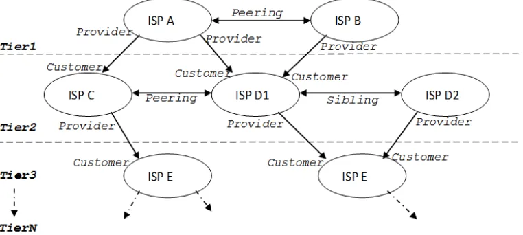
Figure 4.4: Business relationships between ISPs
Figure 4.4 depicts business relationships among ISPs. ISP A and ISP B have peering relationships. For example, ISP A is a provider of ISP C and ISP D1, ISP C is a provider of ISP E, ISP C is a customer of ISP A, ISP D1 and ISP D2 have sibling relationship that ISP D1 and D2 are same organization but having different AS numbers, and ISP D1 has more than one providers: called multi-homing.
The following strategy is applied to identify tiers among ASs: 1. Identify tier-1 AS
2. Identify tier-N AS
• An AS which has tier 1 AS are recognized as tier 2 AS. Then, continue the same approach till reach the last Tier-level. If an AS have multiple providers, multi-homing, (ex, tier 1 and 3 AS), the AS is recognized as lower Tier-level (ex, tier 2 AS)
• If an AS does not have any provider but has peer relationship with tier-N, the AS is recognized as tier-N AS
3. Categorize ASs into two groups (Provider and Access AS)
[image:49.612.198.413.370.554.2]• If a tier-N AS does not have any customer, the AS is categorized as tier-N stub AS
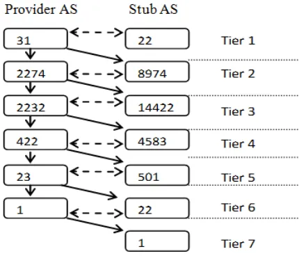
Figure 4.5: Worldwide Internet AS tiers
in the ISP topology, with a single AS in tier 7. The majority of ASs are in tiers 2 and 3, accounting for nearly 83.2% of the ASs in the world. At tier 1, there are a total of 53 AS, of which 31 support customers and 22 who do not support any customer AS. This is around 0.16% of the total number of AS recorded by CAIDA. The tier 1 ASs are Level 3, AT&T and Verizon to name a few.
4.1.3
Nesting, Decoupling, and Floating Properties
Defining network clouds such as the set of backbone or border routers inside an ISP or AS network cloud is called a nesting of clouds. The network clouds defined within the ISP network or AS can also be associated with tiers defined within the ISP network cloud or AS cloud. For example, ISP has several POPs in Figure 4.1. In a magnified view of the POP on the right side of Figure 4.1, the network cloud comprising backbone routers can be associated with tier 1, the network cloud comprising distribution routers can also be associated with tier 2 inside the ISP network, and the network cloud comprising access routers can be associated to tier 3. Thus, a fresh set of tiers is started within a network cloud. This constitutes a nesting of tiers.
CloudAddr once they have an agreement with the concerned service providers. The architecture is thus named the Floating Cloud Tiered (FCT) architecture.
4.2
Tiered Routing Address (TRA)
[image:51.612.133.482.493.636.2]To efficiently use the tiered structure for packet forwarding and internetwork-ing operations a tiered routinternetwork-ing address (TRA) was introduced. TRA allocation depends on the tier level in a network and carries the tier value explicitly as the first field. The tier levels can be assigned as described above. In an ISP, routers closer to a backbone or default gateway have lower tier value and routers near the network edge have higher tier value. TRA can be allocated to a network cloud (that comprises of a set of routers used for a specific purpose, such as backbone, distributions and so on) or a router. They are however not allocated to a network interface. Network interfaces are identified by port numbers. However, a router or end node can have multiple TRAs based on its connection to several upper tier routers or networks. This helps to support multi homing.
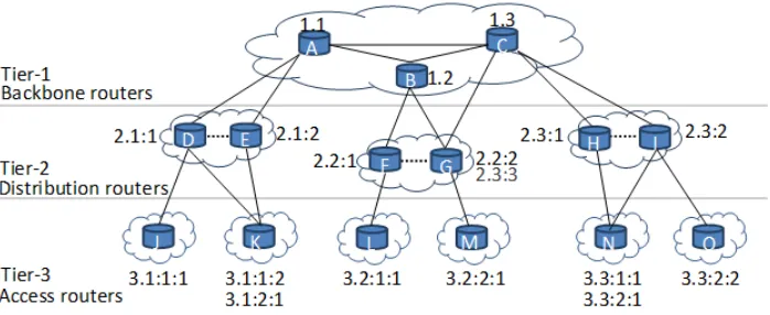
For example, three tiers are identified in the stub network of Figure 4.6, where each tier is allocated a TierValue (TV) from 1 to 3. TRA addresses are noted next to each router. TRA addresses start with a TierValue followed by : (colon) to separate the TreeAddress (TA). The . (dot) notation in the tiered address separates TierValue and TreeAddress. Address allocation starts from the routers at tier 1. Routers A, B, and C at tier 1 are allocated tier addresses
{1.1}, {1.2} and {1.3} respectively. Note that tiered address assignment in TRP isfor a router, andnot for each interface in the router. This has advan-tages such as, reduced number of addresses, reduced routing table size, and ease in addition and removal of routers in the network.
The TreeAddresses of routers at tier 2 are allocated based on the TAs of their directly connected parent network node. In this study, it was assumed that all distribution routers have a link to one or more backbone routers, which may not always be the case. Due to the parent-child relationship between Routers A and D, Router D’s TreeAddress is allocated by taking Router A’s TreeAddress and appending a unique identifier for Router D. Hence, tiered address of Router D following the format {TierValue.TreeAddress} is{2.1:1}, where the first field in the TreeAddress is A’s identifier and the second field is a unique identifier allocated to D by A. Likewise, Router E gets a unique identifier ’2’ from Router A and its tiered address is {2.1:2}. A link between routers which share a common parent is called a trunk-link. Links between Routers D-E, F-G, and H-I are trunk-links, and are represented with dotted lines in Figure 4.6.
has addresses{2.2:2 and 2:3:3}. When a router with multiple addresses has to allocate an address to a child router, it uses one of its addresses as a primary address and allocates an address to its child using the primary address. (This is an assumption made in this study, but can be relaxed or changed depending on the administrative policies within the AS) Thus, Router M that is a child of Router G has one TRA address {3.2:2:1}, where Router G decided to use its address{2.2:2}as the primary address. Decisions for selecting the primary address can be based on metrics of links associated with each address. Multiple addresses are useful for traffic engineering and for immediate recovery from link/node failure to reroute using the alternate address.
The logical view of tiered addressing in Figure 4.6 indicates a tree-like rela-tionship where a tree is rooted at a tier 1 router. Hence the packet forwarding paths do not have loops and the address always refers to the shortest path to tier 1 as configured in this topology.
4.2.1
Nested TRA
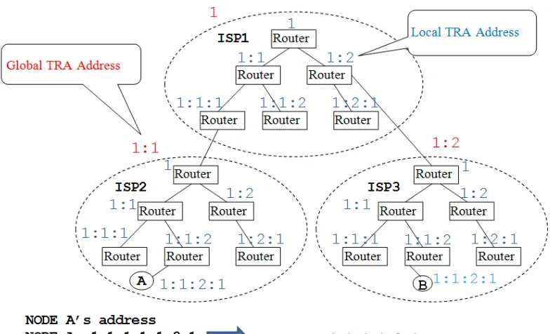
Figure 4.7: Example of Nested TRAs
not affect to any node in ISP2 and 3 because address and topology information are summarized in the global TRA address of ISP1, which is not changed.
4.2.2
TRA Address Format
Figure 4.8: Address Format in FCT Packet
4.3
Tiered Routing Protocol (TRP)
We proposed new routing protocol that uses the tiered routing address (TRA) and adopts tiered based packet forwarding is called Tiered Routing Protocol (TRP). Operations of the TRP include TRA allocation, populating routing tables, packet forwarding, link / node failure detection and recovery.
4.3.1
TRA Allocation Process
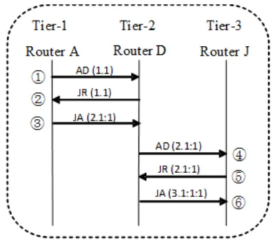
[image:56.612.204.402.443.618.2]TRP allows automatic address allocation by a direct upper tier cloud or node. Once tier 1 nodes acquire their TRAs (or have been assigned their TRAs, tier 2 nodes will get their TRA from the serving tier 1 node.
The process starts from the top tier i.e. tier 1. A tier 1 node advertises its TRA to all its direct neighbors. A node, which receives an advertisement, sends an address request and is allocated an address. For example in Figure 4.9, Router A with TRA 1.1 sends Advertisement (AD) packets to Routers B, C, D, and E. Routers D and E send Join Request (JR) to Router A because they do not have a TRA yet. Router B and C do not request address to Router A because they are at the same tier level. Router A allocates a new address (2.1:1) to Router D using a Join Acceptance (JA) packet. Another new address (2.1:2) is allocated to Router E. The last digit of the new address is maintained by the parent router i.e. Router A. Once Router D registers its TRA, it starts sending AD packets to all its direct neighbors and address assignment continues to the edge routers.
If a router has multiple parents, like Router G in Figure 4.6, it can get multiple addresses. A router with multiple addresses may decide to use one address as its primary address to allocate addresses to its children routers.
4.3.2
Populating Routing Tables
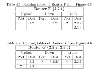
Router F has three different types of links to Routers B, G, and L on port numbers 1, 2, and 3 respectively. Advertisement from Router B is received at port 1 and compared with the tier level of Router B (which is 1) and its own tier level (which is 2). Since tier level of Router B is less than tier level of Router F, the link connected on port number 1 is recognized as up-link and the information is stored in the up-link table. Likewise information about Router G is stored in the trunk-link table, and information about Router L is stored in the down-link table.
Table 4.1: Routing tables of Router F from Figure 4.6
Router F {2.2:1}
Uplink Down Trunk Port Dest Port Dest Port Dest
1 1.2 3 3.2:2:1 2 2.2:2 2.3:3 Table 4.2: Routing tables of Router G from Figure 4.6
Router G {2.2:2, 2.3:3}
Uplink Down Trunk Port Dest Port Dest Port Dest
1 1.2 3 3.2:2:1 4 2.2:1 2 1.3
In Table 4.1 and 4.2, the port column shows the port number of the router and dest column shows the TRA of direct neighbor obtained from the adver-tisements. There are multiple entries against a single port in the trunk-link table of Router F because Router G has two TRAs. The routing table for Router G is also shown.
hence there is least delay in populating the routing tables. The initial con-vergence time in TRP is significantly lower as just one advertisement packet is required from a connected neighbor. Due to these features, the number of control packets exchanged for updating routing information is very low.
4.3.3
Packet Forwarding
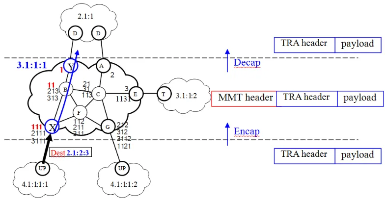
For a source node to send a packet to a destination node, the source node calculates a forwarding address. First, the TierValue of a common parent between itself and the destination node is calculated. For this purpose, the source node compares its tree address with the destination address. Assume that the source node is Router L and destination node is Router M in Fig-ure 4.6. Router L compares {3.2:1:1}with {3.2:2:1}, from left to right to find the TierValue of a common parent. The only common part in these addresses is the first field after the TierValue, thus the common parent is available only at tier 1, i.e. the TierValue of a common parent is {1}. The calculated Tier-Value will be the TierTier-Value in the forwarding address. Next, the TreeAddress in the forwarding address is the TreeAddress of the destination node from the point where the common value is obtained. Thus, the forwarding address is
{1.2:2:1}. As another example, a forwarding address between source Router J
{3.1:1:1}and the destination Router K{3.1:1:2}will be {2.1:2}because tier 1 and 2 of source and destination address are the same {1:1}, thus the TreeAd-dress of the forwarding adTreeAd-dress starts with tier 2 adTreeAd-dress of the destination
Algorithm 1Packet forwarding at router R and incoming packet P
if R.T ierV alue==P.T then
if R.T A.last tier == P.T A.1st tier then
if port=f ind(P.T A.2nd tier, downlink table) then
remove(P.T A.1st tier)
P.T V ←P.T V + 1
f orward(P, port)
returntrue
end if
else if R.T V == 1 then . at Tier 1
if port=f ind(P.T A.1st tier, uplink table) then
f orward(P, port)
returntrue
end if
else if R.T V −P.T V == 1 then
if R.T A.parent tier== P.T A.1st tier then
if port=f ind(P.T A.2nd tier, trunklink table)then
remove(P.T A.1st tier)
P.T V ←P.T V + 1
f orward(P, port)
return true
end if end if
else if R.T V < P.T V then
discard(P) . wrong packet
return f alse
end if end if
if port=f ind(uplink table) then
f orward(P, port)
return true
end if
discard(P) . no entry in routing tables
returnf alse
code for the forwarding process at a TRP router is provided in Algorithm 1. In Algorithm 1, R represents the router that processes the packet, P represents the incoming packet, TV and TA represent TierValue and TreeAddress in the tiered addresses that is associated to R and P. For example, a packet containing the forwarding address{1.2:2:1}from Router L is sent to Router F. At Router F, it compares TierValue of the forwarding address {1} and its own TierValue of {2}. Since the TierValue of the forwarding address is smaller than Router F’s value, a packet is forwarded upwards. A packet will be forwarded upwards until it reaches the same TierValue. In this case, a packet reaches Router B
{1.2}. Then, Router B increments TierValue of the forwarding packet by 1 and removes the first TierValue{2}. The forwarding address is now{2.2:1}. From this forwarding address, Router B knows which down link port to forward the packet (which is port{2}). Thus, the packet is forwarded to Router G{2.2:2}. Router G makes the same forwarding decision of comparing the TierValue, then incrementing by 1, removing the first TierValue of the forwarding packet, which results in {3.1}. Finally the packet is forwarded to Router M. The packet takes a path of Routers L-F-B-G-M. There is another option to take the path Routers L-F-G-M because Router F could be made aware of trunk-link connection from its routing table.
4.3.4
Failure Detection and Handling
times, the TRP router updates its routing table accordingly. However, in TRP packet forwarding on link/node failure a router does not have to wait for the 4 missing AD packets. An alternate path, if it exists, can be used immediately on the missing a single AD packet irrespective of the routing table update. With the current high speed and reliable technologies, it is highly improba-ble to miss AD packets and redirecting packets on missing one AD packet is justified. However for a fair comparison with OSPF we adopted the 4 missing hallo packets to indicate a link/node failure.
Up-link Failure
If a node detects an uplink failure and has a trunk link, it can use the trunk link, because trunk link exists between routers that have the same parent route, or it can use an uplink is one exists. In Figure 4.10, the sibling router connected to Router F derives its address from the same parent. So, Router F knows that the uplink router on Router G will be its parent Router B.
Figure 4.11: Failure handling with down-link
Figure 4.12: Trunk-link information sharing by the parent router
Down-link Failure
as described in Figure 4.12. Due to inheritances, routers can assume responsi-bilities to forward for to their directly connected neighbors as the TRAs carry relationship information.
Figure 4.13: Address changes in TRP
Address Changing
Figure 4.14: Primary address change
Primary Address Changing
If a node has multiple addresses and a link to a primary address failed, the node changes one of its secondary address to primary address and advertises the same. The child of the node also changes its address in the same manner as described in the case above and keeps the last digit. For example, Router G has two addresses and let 2.2:2 be the primary address in Figure 4.14. When a failure occurs between Routers B and G, Router G changes its primary address to 2.3:3 and then advertises it. As the result, Router M changes its address to 3.3:3:1.
4.4
Integration of Inter and Intra Domain
Routing
this section, we show possibility of integration between TRP and other rout-ing protocol that TRP as inter-domain and another as intra-domain routrout-ing protocol.
4.4.1
MMT Routing in a Cloud
As part of our research we also investigated a robust routing scheme to be used for intra-cloud routing called Multi-Meshed Tree (MMT) routing [64]. Within a cloud, if we can grow trees, whose branches can be meshed and rooted at nodes that are either connected to an uplink cloud or a sibling cloud we will be able to forward the packets across the clouds. The growth of the tree is meshed yet loop free because of the numbering scheme used to generate the virtual IDs (VIDs) assigned to the nodes. The VIDs carry the branch information and also the route information to and from the root node. The meshed trees are created using local computations, in a distributed fashion and has very low complexity and overhead, hence is very robust.
Figure 4.15: Example of MMT (Hop limit is 3)
this example. Since each node allows having multiple VIDs, nodes in the tree can have redundant routes to the CH. To avoid loops in trees, VIDs are not assigned if there is already a child-parent relationship with particular VID. For example, if a node has VID 121, and joining node already has VID 12, the joining node will not request to get VID 1211. This VID acceptance rule applies for direct parent-child as well as any grandparents or grand children.
Figure 4.16: 3-ways Handshake in MMT Joining Process
Figure 4.16 describes the 3-ways handshake for meshed tree creation. Node B advertise its VID (11) through AD (Advertisement) packet to Node C, then Node C wants to join and sends JR (Join Request) packet for the VID (11) to Node B, Node B assigns new VID (111) for Node C and sends JR to Cluster Head (CH), then Cluster Head makes decision and sends JA (Join Acceptance) to node B, node B sends JA to node C, and node C updates its VID list. Now node C joins Cluster Tree. In figure 6, the ID of each node represents how MMT works to assign VIDs for nodes in one tree. Children inherent VIDs from parents and get adjunctive ID assigned by parents.
Figure 4.17: Data Forwarding with MMT
4.5
TRP Code and Local Testbed
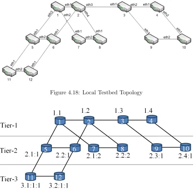
Figure 4.18: Local Testbed Topology
Figure 4.19: Local Testbed Topology with Example TRAs
Chapter 5
Evaluation of TRA and TRP
To evaluate the FCT architecture, we first validated tiered stricture in an ISP and among ISPs discussed in Chapter 4.1.1 and 4.1.2 by using realistic datasets of Internet topologies. Then we first evaluate TRA with router-level topology of an ISP and AS-level topology of the Internet. Next, to validate the operation of TRP, a Linux-based FCT router is implemented. With the FCT router, the performance of the TRP is compared with both intra- and inter-domain routing protocols.
5.1
Evaluation of TRP in Intra-domain
Rout-ing
5.1.1
Analyzing AT&T Network
Figure 5.1: US AT&T network in OPNET imported from Rocketfuel data With AT&T network data, we identified a total of 11,403 routers with 13,689 links interconnecting them (excluded Hawaii and Alaska). Figure 5.2 shows router-level topology of the entire AT&T network in the US. Figure 5.1 shows the topology imported into the OPNET network simulation tool [66] including the geographical locations of the different POPs (cities).
There were a total of 110 POPs in the AT&T network which can be seen as dots in the Figure 5.1. The numbers on the links represent the number of phys-ical connections between POPs. Figure 5.3 and 5.4 are enlarged views of New York area and San Francisco area from the AT&T network. As seen in those figures, topology between cities (POPs) are look like hub and spoke topology, but inside of each city (POP) is highly connected like meshed topology.
Figure 5.2: AT&T Router-Level Network Topology
Figure 5.3: AT&T Router-Level Network Topology (NY area)
Figure 5.4: AT&T Router-Level Network Topology (SF area)
The next step was in identifying tiers and clouds inside every POP in the AT&T network. BB routers are assigned to a tier 1 cloud in the POP. The DR routers were designated to be at tier 2, and AR routers at tier 3. After assigning such categorization to all 11,403 routers, the TRA address was allocated to every router in entire AT&T network as explained in Chapter 4.2. Figure 5.7 shows sorted distribution of routers in each POP and exact numbers are presented in Table 5.1. Only 10 % of AT&T POP has large number of routers and 90 % od them are less than 230 routers, which represents property of a hub-and-spoke topology. Those 10 % of large POPs can be recognized as a backbone of backbone in AT&T network and it can also be recognized as another tier in the network.
con-Table 5.1: Number of Routers at each POP in AT&T
CITY (POP) NUM CITY (POP) NUM CITY (POP) NUM 1 Chicago, IL 1010 41 Pittsburgh, PA 68 81 San Bernadino, CA 32 2 New York, NY 946 42 Harrisburg, PA 67 82 Des Moines, IA 31 3 Washington, DC 576 43 Wayne, PA 66 83 Dunwoody, GA 31 4 Atlanta, GA 499 44 Nashville, TN 66 84 San Antonio, TX 30 5 Dallas, TX 495 45 Hartford, CT 65 85 Ojus, FL 30 6 San Francisco, CA 485 46 Oklahoma City, OK 65 86 Bridgeport, CT 28 7 Seattle, WA 393 47 Rochelle Park, NJ 58 87 Portland, ME 27 8 Orlando, FL 368 48 Galva, IL 57 88 Fort Worth, TX 26 9 Cambridge, MA 368 49 Santa Clara, CA 57 89 Memphis, TN 26 10 Los Angeles, CA 337 50 Tampa, FL 56 90 Camden, NJ 26 11 Denver, CO 321 51 Omaha, NE 56 91 Madison, WI 25 12 St Louis, MO 226 52 Silver Springs, MD 55 92 Manchester, NH 25 13 Philadelphia, PA 205 53 Syracuse, NY 51 93 Rochester, NY 23 14 Phoenix, AZ 181 54 Cincinnati, OH 50 94 Norfolk, VA 23 15 Detroit, MI 178 55 Baltimore, MD 47 95 Dayton, OH 22 16 San Diego, CA 174 56 Birmingham, AL 44 96 Colorado Springs, CO 22 17 Houston, TX 159 57 Florissant, MO 44 97 Louisville, KY 19 18 Cleveland, OH 131 58 Tulsa, OK 43 98 Brookhaven, MI 18 19 Austin, TX 126 59 Spokane, WA 43 99 Freehold, NJ 16 20 New Brunswick, NJ 115 60 Richmond, VA 43 100 Akron, OH 16 21 White Plains, NY 107 61 Hamilton Square, NJ 42 101 Little Rock, AR 16 22 Salt Lake City, UT 106 62 Greensboro, NC 42 102 Madison Heights, VA 15 23 Anaheim, CA 100 63 Buffalo, NY 42 103 Worcester, MA 15 24 Arlington, VA 98 64 Plymouth, MI 40 104 Bridgeton, MO 14 25 San Jose, CA 94 65 Fort Lauderdale, FL 40 105 West Palm Beach, FL 10 26 Charlotte, NC 91 66 Oakland, CA 39 106 Abingdon, VA 5 27 Indianapolis, IN 85 67 Jacksonville, FL 39 107 Champaign, IL 2 28 Cedar Knolls, NJ 85 68 Providence, RI 39 108 Palo Alto, CA 1 29 Miami, FL 82 69 Albuquerque, NM 39 109 Newark, NJ 1 30 Riverside, CA 81 70 Columbia, SC 38 110 Tucson, AZ 1 31 Minneapolis, MN 81 71 Davenport, IA 38
[image:75.612.114.503.168.600.2]Figure 5.5: AT&T Router Degree Distribution
nectivity and address allocation study to the POP level within an ISP i.e. the AT&T ISP.
Figure 5.6: AT&T Router Shortest Path Length Distribution
cloud. If a DR router is on the path to different BB routers, then the DR router chooses the shorter hop to a BB router, and is considered to belong to the distribution cloud under that BB router.
5.1.2
Tiered Structure and TRA allocation
Figure 5.7: US AT&T POP Distribution
all BB routers thus belong to the cloud, which has TRA {1.7}. As per our study we used integers between 1 and 110 to uniquely identify each POP in the AT&T network and 7 is the Seattle POP ID assigned by us (one could use any other numbering strategy). At tier 2, there are 94 DR routers and 17 clouds as identified. Each block of dots (i.e. routers) at tier 2 in the figure represents a cloud. At tier 3, there are 293 AR routers and hence 293 clouds because each AR router is recognized as a cloud for reasons stated earlier, hence each dot is a cloud.
Figure 5.8: BB Routers Distribution of AT&T Network
largest BB cloud and the highest number of DR routers. The Dallas POP has the largest distribution cloud with 56 routers. The Seattle POP has the maximum number of AR routers which are connected to the same distribution cloud. These statistics are provided to show that they can be used to identify and optimize the proper size of a single cloud, help in nesting cloud decision.
5.1.3
Address Length and Numbers
Figure 5.9: Correlation between BB routers and POP size can be calculated by the following equation 5.1:
T RAlen=T Vlen+LFend+ T V
X
i=1
(LFlen+T Aleni) (5.1)
T Aleni=
4 (1< T A <16) 8 (16 < T A <256) 12 (256 < T A <4096)
where T V is tier value of a TRA address, T Alen is a length of TA filed at
the tier ilevel, T Vlenis a length of a TV field, which is fixed 6 bits, andLFlen
Figure 5.10: Seattle POP Topology of AT&T Network
Figure 5.11: Seattle POP Topology of AT&T with FCT model
Table 5.2: AT&T Network Statistics based on Tiered Routing Addresses Total number of routers 11,403
Total number of links 13,689 Total number of POPs 110 Total number of BB routers 389 Total number of DR routers 6,395 Total number of AR routers 4,619 Maximum TreeAddress at tier 1 110 POPs Maximum TreeAddress at tier 2 429 (New York) Maximum TreeAddress at tier 3 99 (Seattle)
Maximum POP size 1,010 (Chicago POP) Maximum BB cloud size 44 routers (New York POP) Maximum DR routers in a POP 542 routers (New York POP) Maximum distribution could size 56 routers (Dallas POP)
Figure 5.12: TRA Address Length distribution across AT&T network address per router similar to Network Service Access Point (NSAP) addresses in Intermediate System to Intermediate System (ISIS).
Figure 5.13: Total Size of TRA and IP Addresses
Figure 5.14: Total Number of Allocated TRA and IP Addresses
for all the routers in the AT&T using IP (v4 or v6) addresses and the tiered addresses. Both statistics shows that TRA address requires less number of address and size, which can also reduce traffics in the Internet.
5.1.4
HD Ratio for Address Allocation Efficiency
The tiered addressing scheme allows a maximum of 212n addresses at tier level
can be calculated using Equation 5.2.
AL = 14n+ 6 (5.2) where
• AL: Maximum address length
• n: Total number of the tiers in the network
In the current Internet, the efficiency of the IP address assignment was analyzed with the Hratio as given by Equation 5.2 [67].
Hratio =
log10(NAO)
NAB
(5.3) where
• NAO: Number of allocated objects
• NAB: Number of available bits
However, since Equation 5.3 did not count the multiplicative affect of the loss of efficiency at each level of a hierarchical plan, we decided to use the Host Density ratio (HDratio), which is adopted to analyze IPv6 address allocation
efficiency by IETF [67] and is given in Equation 5.4.
HDratio =
logx(NAO)
logx(M AX NAO)
(5.4) where
• x: Any integer value bigger than 0
In [68], a HDratio of 0.94 is identified as the utilization threshold for IPv6
address space allocations. Equation 5.4 can this be rewritten to actually find out theNAO as in Equation 5.5.
NAO = (M AX NAO) HDratio
(5.5) According to Equation 5.5, IPv6 reachesHDratio of 0.9 when 1.65931E+36
[image:85.612.116.499.324.555.2]addresses are allocated to the objects. At this, point new address space will be required for the new nodes.
Table 5.3: Number of Nodes in each Tier Level Tier
value
Max address length
Address capac-ity at the tier
Total capac-ity of network
Network capac-ity at HD:0.94 1 20 4096 4096 2486.671123 2 34 16777216 16781312 6184952.337 3 48 68719476736 68736258048 15379943237 4 62 2.81475E+14 2.81544E+14 3.82449E+13 5 76 1.15292E+18 1.15320E+18 9.51024E+16 6 90 4.72237E+21 4.72352E+21 2.36488E+20 7 104 1.93428E+25 1.93475E+25 5.88069E+23 8 118 7.92282E+28 7.92475E+28 1.46233E+27 9 132 3.24519E+32 3.24598E+32 3.63634E+30 10 146 1.32923E+36 1.32955E+36 9.04239E+33 11 160 5.44452E+39 5.44585E+39 2.24854E+37 12 174 2.23007E+43 2.23062E+43 5.59139E+40 13 188 9.13439E+46 9.13662E+46 1.39040E+44
address fields of 12 bits each. The total number of supported addresses, for a given TierValue including all of the addresses within the tiered hierarchy is given in the fourth column. Let us explain this with an example: at tier 2 we have a maximum address space given by 16,777,216 (=212n, wheren = 2).
However there are addresses supported in tier 1 under which we have tier 2. So the total number of addresses that can be supported in a system that has 2 tier levels will be given by 16,781,312, which is 4096 (at tier 1) + 16,777,216 at tier 2. So the values in column 4 are a cumulative count of addresses from all tiers above a given tier, including that tier. The total number of addresses that can be supported by the network till it reaches the HD ratio of 0.94 was calculated using Equation 5.5 and is given in the last column.
As it is seen in Table 5.3, the tiered routing addresses reach the IPv6 address allocation threshold capacity at tier 11 with 160 bits of address length at most. However, the threshold in the tiered address is not fixed as for IPv6; it is flexible and can be extended as needed by increasing the tier value. The only restricting factor could be the address length. As explained under the packet forwarding section and along with the nested concepts, the maximum address length that any router has to deal with is determined by the first address field in the tiered addresses, which knows how to direct or forward a packet.
of the tiered address would preclude MAC addresses and that all forwarding whether inter or intra-cloud can be supported by the tiered address.
In this TRA validation, the main goal was to support for future growth in an unrestricted manner, whether it is in terms of address space or net-works. We highlighted the efficient use of address space with the tiered address scheme. We provided some operational aspects of the internetworking model to explain the application of the tiered addresses. We also illustrated tier based address aggregation with examples and applied the same to the AT&T network in the US. Using this application and the HDratio we then analyzed
some performance characteristics of the tiered addressing scheme.
5.1.5
Routing Table Size Analysis of TRP
We now provide an example of applying the FCT model to a small network of 6 routers with 9 network segments. We provide the routing tables, when the network uses IP addresses and runs an IP routing protocol, and compare with the routing table sizes that can be expected if the network were running TRP.
Table 5.4: IP Routing Table of Router B in Figure 5.15
Destination Network Route Via
10.1.1.0 connected 10.1.2.0 connected 10.1.3.0 10.1.4.0, 10.1.1.0 10.1.4.0 connected 10.1.5.0 10.1.2.0, 10.1.4.0 10.1.6.0 10.1.4.0 10.1.7.0 10.1.4.0 10.1.8.0 10.1.2.0 10.1.9.0 10.1.2.0, 10.1.4.0
Figure 5.15: A Sample IP network Topology with 9 Subnets
routing table at any one of the routers will be similar to that shown for router B in Table 5.4. This table has 9 entries for the 9 segments, assuming that the tables are fully populated with all network segment addresses without depending on default forwarding addresses.
Without loss of generality, the routing tables for the above network was populated using Routing Information Protocol (RIP). Running OSPF or BGP, (as would be normally expected for inter-domain routing), would have resulted in routing tables of similar size. For the network as shown in Figure 5.15, and with routers having a minimal number of interfaces, requires a routing table with 9 entries.
only two entries. Routers E and F will have two and three entries respec-tively. That is irrespe