A comparison of iterative and DFT-based polynomial matrix eigenvalue decompositions

(1)

A Comparison of Iterative and DFT-Based

Polynomial Matrix Eigenvalue Decompositions

Fraser K. Coutts

∗

, Keith Thompson

∗

, Ian K. Proudler

∗,†

, Stephan Weiss

∗

∗ _{Department of Electronic & Electrical Engineering, University of Strathclyde, Glasgow, Scotland} † _{School of Electrical, Electronics & Systems Engineering, Loughborough Univ., Loughborough, UK}

{fraser.coutts,keith.thompson,ian.proudler,stephan.weiss}@strath.ac.uk

Abstract—A variety of algorithms have been developed to com-pute an approximate polynomial matrix eigenvalue decomposition (PEVD). As an extension of the ordinary EVD to polynomial matrices, the PEVD will generate paraunitary matrices that diagonalise a parahermitian matrix. This paper compares the decomposition accuracies of two fundamentally different meth-ods capable of computing an approximate PEVD. The first of these — sequential matrix diagonalisation (SMD) — iteratively decomposes a parahermitian matrix, while the second DFT-based algorithm computes a pointwise in frequency decomposition. We demonstrate through the use of examples that both algorithms can achieve varying levels of decomposition accuracy, and provide results that indicate the type of broadband multichannel problems that are better suited to each algorithm. It is shown that iterative methods, which generate paraunitary eigenvectors, are suited for general applications with a low number of sensors, while a DFT-based approach is useful for fixed, finite order decompositions with a small number of lags.

I. INTRODUCTION

Broadband multichannel problems can be expressed using polynomial matrix representations [1]. Such formulations can be used in a number of areas, including broadband angle of arrival estimation [2], [3], polyphase analysis and synthesis matrices for filter banks [4], and broadband beamforming [5], [6]. These problems typically involve parahermitian poly-nomial matrices, which are identical to their parahermitian conjugate, i.e.,R₍_z_{) =}R˜₍_z_{) =}RH₍₁_/z∗₎_{[4]. Such a matrix} R₍_z₎_{can arise as the}_z_{-transform of a space-time covariance}

matrix R[τ].

A polynomial matrix eigenvalue decomposition (PEVD), which is an extension of the eigenvalue decomposition to parahermitian matrices, has been defined in [7]. The PEVD uses finite impulse response (FIR) paraunitary matrices [8] to approximately diagonalise a space-time covariance matrix. Given an input parahermitian matrix R₍_z₎_∈CN×N_{, and its} associated coefficient matrixR[τ], PEVD algorithms generate an output diagonal matrixD₍_z₎_{containing eigenvalues, and a}

paraunitary matrix F₍_z₎_{containing eigenvectors, such that} D₍_z₎_≈F₍_z₎R₍_z₎F˜₍_z₎_. ₍₁₎

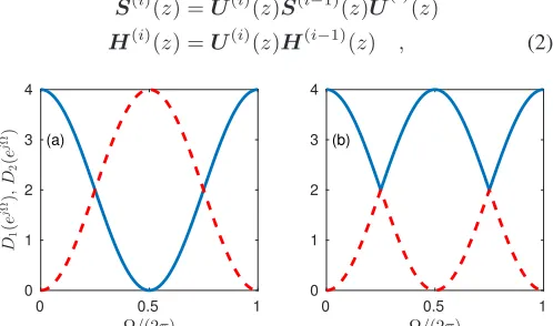
Equation (1) has only approximate equality, as the PEVD of a finite order polynomial matrix is generally not of finite order. Existing PEVD algorithms include sequential matrix di-agonalisation (SMD) [10], second-order sequential best ro-tation (SBR2) [7], and various evolutions of the algorithm families [11]–[13]. Each of these algorithms uses an iterative approach to approximately diagonalise a parahermitian matrix, and in many cases they encourage spectral majorisation [9], such that the resulting eigenvalues are ordered, as shown for the example of a 2×2matrix in Fig. 1.

A DFT-based PEVD formulation, which transforms the problem into a pointwise in frequency standard matrix

decom-position, is provided in [14]. The method can either return a spectrally majorised decomposition, akin to the example in Fig. 1(b), or attempt to compute smooth, ideally analytic, eigenvalues as shown in the example of Fig. 1(a). The inherent drawback of a lack of phase-coherence between independent frequency bins [15] is solved via a quadratic nonlinear min-imisation problem, which encourages phase alignment between adjacent bins.

As both iterative and DFT-based PEVD algorithms reach a solution to (1) through different methodologies, a comparison of their decomposition performance is of interest. Here, we compare the decompositions of SMD — as a representative of iterative PEVD algorithms — and the DFT-based approach in terms of algorithmic complexity, reconstruction error, eigen-vector paraunitarity and order, parahermitian matrix diagonali-sation, and spectral majorisation. Through this comparison, we obtain results that indicate the type of broadband multichannel problems that are better suited to each algorithm.

Below, Sec. II and Sec. III will provide a brief overview of the SMD and DFT-based algorithms from [10] and [14]. A comparison of the decomposition accuracies is presented in Sec. IV, with conclusions drawn in Sec. V.

II. SEQUENTIALMATRIXDIAGONALISATION A. Overview

The SMD algorithm approximates the PEVD using a series of elementary paraunitary operations to iteratively diagonalise a parahermitian matrix R₍_z₎_∈CN×N_.

Upon initialisation, the algorithm diagonalises the lag-zero coefficient matrix R[0] by means of its modal matrix Q(0); i.e.,S(0)₍_z_{) =}Q(0)R₍_z_)Q(0)H_{. The unitary}Q(0)— obtained from the EVD of the lag-zero slice R[0]— is applied to all coefficient matrices R[τ]∀τ, and initialisesH(0)₍_z_{) =}Q(0)_.

In theith step,i= 1,2, . . . I, the SMD algorithm computes

S(i)₍_z_{) =}U(i)₍_z₎S(i−1)₍_z₎U˜(i)₍_z₎

H(i)₍_z_{) =}U(i)₍_z₎H(i−1)₍_z₎ _, ₍₂₎

0 0.5 1

Ω/(2π)

0 1 2 3 4

D1

(

e

j

Ω), D2

(

e

j

Ω) (a)

0 0.5 1

Ω/(2π)

0 1 2 3 4

[image:1.612.322.571.564.711.2]

(b)

(2)

in which

U(i)₍_z_{) =}Q(i)Λ(i)(z). (3) The product in (3) consists of a paraunitary delay matrix

Λ(i)(z) = diag{1 . . . 1

| {z }

k(i)₋₁

z−τ(i) 1 . . . 1

| {z }

N−k(i)

} , (4)

and a unitary matrix Q(i)_{, with the result that} _U(i)₍_z₎

in (3) is paraunitary. For subsequent discussion, it is convenient to define intermediate variablesS(i)′₍_z₎_andH(i)′₍_z₎_where

S(i)′₍_z_{) =}Λ(i)(z)S(i−1)₍_z₎Λ˜(i)(z)

H(i)′₍_z_{) =}Λ(i)(z)H(i−1)₍_z₎ _, ₍₅₎

and

S(i)₍_z_{) =}Q(i)S(i)′₍_z_)Q(i)H _. ₍₆₎

Matrices Λ(i)(z) and Q(i) are selected based on the position of the dominant off-diagonal column in

S(i−1)₍_z₎_•_—_◦S(i−1)[τ], as identified by the parameter set {k(i), τ(i)}= arg max

k,τ kˆs

(i−1)

k [τ]k2 , (7)

where

kˆs(_ki−1)[τ]k2=

q PN

m=1,m6=k|s

(i−1)

m,k [τ]|2 (8)

and s(_m,ki−1)[τ] represents the element in the mth row and kth column of the coefficient matrix at lagτ,S(i−1)[τ].

The shifting process in (5) moves the dominant off-diagonal row and column into the zero lag coefficient matrix

S(i)′_[0]_{. The off-diagonal energy in the shifted row and column}

is then transferred onto the diagonal by the unitary matrixQ(i)

in (6), which diagonalises S(i)′[0] by means of an ordered EVD.

Iterations continue forI steps until S(I)₍_z₎_{is sufficiently}

diagonalised with dominant off-diagonal column norm

max

k,τ kˆs

(I)

k [τ]k2≤ǫ , (9)

where the value of ǫ is chosen to be arbitrarily small. On completion, SMD generates an approximate PEVD given by

D₍_z_{) =}S(I)₍_z_{) =}F₍_z₎R₍_z₎F˜₍_z₎_, ₍₁₀₎

whereF₍_z₎_{is a concatenation of the paraunitary matrices:} F₍_z_{) =}H(I)₍_z_{) =}U(I)₍_z₎_{· · ·}U(0)₍_z_{) =}

I

Y

i=0

U(I−i)₍_z₎_.

B. Algorithm Complexity

At theith iteration of SMD, every matrix-valued coefficient in S(i)′₍_z₎ _{must be left- and right-multiplied with unitary}

matrix Q(i); similarly H(i)′₍_z₎ _{is left-multiplied with} Q(i). A total of 2L(i) _and_L(i)

H matrix multiplications are therefore required to update S(i)′₍_z₎_andH(i)′₍_z₎_{, which have lengths}

L(i)_and_L(i)

H . Assuming that the complexity of the

multiplica-tion of twoN×N matrices is of orderO(N3₎_{; the complexity}

of one SMD iteration is of order O(N3₍₂_L(i) ₊_L(i) H)) ≈

O(N3_L₎_{, if it is assumed that} _L(i) _and_L(i)

H are proportional

to the length,L, of the input parahermitian matrix.

The update step dominates the complexity of SMD [10]; thus, the algorithm complexity is of orderO(N3_L₎_.

III. DFT-BASEDPEVD

A. Overview

The approach in [14] uses a decomposition of the form

R[k] =FH[k]D[k]F[k], k= 0,1, . . . , K−1, (11) where F[k]contains eigenvectors, D[k] contains eigenvalues, andR[k]is obtained from theK-point DFT ofR[τ],

R[k] =R₍_z₎_|_z₌_wk K =

Pτmax τminR[τ]w

kτ

K , k= 0,1, . . . , K−1, where wK = e−j2π/K. An approximate PEVD is therefore obtained via K EVDs that are pointwise in frequency.

The PEVD in (1) corresponds to linear convolution in the coefficients domain; however, the decomposition obtained in the DFT domain corresponds to the circular convolution

R[ ((τ))_K] =FH[ ((τ))_K]⊛D[ ((τ))_K]⊛F[ ((τ))_K], (12) where ⊛ _{is the circular convolution operator, and} ₍₍_τ₎₎

K denotes τ modulo K. For (12) to be equivalent to (1), the number of frequency bins must satisfy

K≥(2M+L−2), (13) whereL= (τmax−τmin+ 1)is the length of input

parahermi-tian matrixR₍_z₎_{, and}_M _{is the assumed length of the}

parau-nitary matrix that is non-zero. That is, F[τ] = 0forτ ≥M

and τ <0. Typically, choosingK = (2M +L−2) is valid, as decomposition accuracy does not increase significantly for largerK[14], but algorithmic computational complexity does. At each frequency bin, eigenvalues are typically arranged in descending order; this results in approximate spectral majori-sation of the polynomial eigenvalues. Sec. III-B discusses the rearrangement of eigenvalues to form a smooth decomposition. Each eigenvector in a conventional EVD may be influenced by an arbitrary scalar phase angle and still be valid. This ambi-guity in phase of each eigenvector can lead to discontinuities in phase between adjacent frequency bins. For a short paraunitary matrix F₍_z₎_{, these discontinuities must be smoothed. This}

is achieved through the use of a phase alignment function, described in Sec. III-C, which uses the Dogleg algorithm [16] to solve an unconstrained optimisation problem.

Following phase alignment,F[τ] is computed as

F[τ] =PK_k₌₀−1F[k]w−kτ

K , τ = 0,1, . . . , M−1, (14) and D₍_z₎ _{is the diagonal elements of} F₍_z₎R₍_z₎F˜₍_z₎_{. Any}

energy in lagsτ =M . . . K−1 ofF[τ] is ignored.

B. Smooth Decomposition

If strong decorrelation is required for an application, but spectral majorisation is not, then a smooth decomposition may be preferable. In such a decomposition, the eigenvalues — and their eigenvectors — are arranged such that discontinuities be-tween adjacent frequency bins are minimised. Discontinuities occur when the eigenvalues intersect at some frequencies.

For a smooth decomposition, the eigenvectors in adjacent frequency bins are rearranged using the inner product

cij[k] =fi[k−1]fjH[k], (15) where,fi[k]is theith row ofF[k]. For each eigenvectorfi[k−

1],i= 1. . . N, a subsequent eigenvectorfi′[k]is chosen from

an initial set S={1. . . N}of the rows ofF[k] such that

i′= arg max

j∈S{|cij[k]|}, (16) Oncei′_{is identified, it is removed from the set:}_S₌_S_{− {}_i′_}_,

(3)

The selected eigenvectors are combined in a rearranged matrix F′_[_k_{] = [}_fT

1′[k]. . .fNT′[k]]T, and F[k] is set equal to F′[k]. Thus, the eigenvector discontinuity between F[k−1]

andF[k]has been reduced. This process is completed fork= 1. . . K−1.

C. Phase Alignment

Phase alignment of eigenvectors in adjacent frequency bins is vital for a compact order decomposition. Thus, if a compact order is sought (e.g., here it is desired that only lags

τ = 0. . . M −1 are non-zero), then phase alignment can be achieved by finding the phase changes required for each eigenvector fi[k]∀i, kto enforce this low order.

The phase of the ith eigenvector at frequency bin k can be adjusted by an angleθi[k]according toˆfi[k] =ejθi[k]fi[k]. For the ith polynomial eigenvectorfi[τ] to be compact, it is required to find angles ~θi= [θi[1]. . . θi[K−1]]T, that satisfy

f

i

[

τ

] =

_K1

P

Kk=0−1

f

i

[

k

]

e

jθi[k]

w

−Kkτ

=

0 ,

(17) forτ =M, . . . , K−1. Without loss of generality, letθi[0] = 0. These(K−M)-folded equations can be expressed as

FM(fi)x(~θi) +fM(fi) =0, (18) where x(~θi) = [ejθi[1], ejθi[2], . . . , ejθi[K−1]]T, fM(fi) =

[fi[0],fi[0], . . . ,fi[0]]Tis aN(K−M)×1 vector, and FM(fi) =



    

fT

i[1]w−KM fiT[2]wK−2M . . . fiT[K−1]w−

(K−1)M K

fT

i[1]w−

(M+1)

K fiT[2]w−

2(M+1)

K . . . fiT[K−1]w−

(K−1)(M+1)

K ..

. ... . .. ...

fT

i[1]w−

(K−1)

K fiT[2]w−

2(K−1)

K . . . fiT[K−1]w−

(K−1)2 K



    

is aN(K−M)×(K−1) matrix.

In general, there may exist no phase vector~θi which satis-fies (18). However, by minimising the energy in the coefficients forτ =M, . . . , K−1, some~θi can be obtained. The energy in these coefficients is therefore used as the objective of the unconstrained minimisation problem

J(~θi) =kFM(fi)x(~θi) +fM(fi)k2, i= 1. . . N . (19) Thus,~θi is obtained by solving~θi= arg minJ(~θi). In [14], it was found that the Dogleg method [16] was able to satisfac-torily minimise J(~θi)fori= 1. . . N.

D. Algorithm Complexity

The complexity of each of the N instantiations of the Dogleg method is O(K3) due to matrix inversion [14]; thus, the total complexity of the phase alignment step is of order O(N K3₎_{. Given that} _K _{is bounded from below by}_L_{in (13)}

for constant M, O(N K3₎ _{can be expressed as} _O₍_{N L}3₎_.

The computation of the frequency domain representation of

R[τ] ∀ τ, the execution of K EVDs, and the smoothing of eigenvalues are of lower complexity than this step; thus, the total complexity of the algorithm is approximatelyO(N L3).

IV. ALGORITHMCOMPARISON A. Metrics

Denote the mean-squared reconstruction error for an ap-proximate PEVD as

MSE = _N21_L′ P

τkER[τ]k2F, (20)

where ER[τ] =R[ˆ τ]−R[τ] ∀ τ, Rˆ(z) = F˜(z)D(z)F(z),

L′ _{is the length of} E_R₍_z₎_{, and} _{k · k}_F _{denotes the Frobenius}

norm. Furthermore, define the paraunitarity (PU) error as

η

=

_N1

P

_τ

kE

F

[

τ

]

−

I

N

k

2F

,

(21)

where E_F₍_z_{) =} F₍_z₎F˜₍_z₎_{, and} IN is an N ×N identity

matrix. Finally, define diagonalisation as the ratio of off-diagonal energy in D₍_z₎_{to the total energy:}

E

diag

=

P

τkD¯[τ]k

2 F

P

τkD[τ]k2F

,

(22)

where D[¯ τ] is equal to D[τ] but with its diagonal elements set to zero. The output paraunitary matrix F₍_z₎ _{can be used}

in signal processing applications. A useful metric for gauging the implementation cost of this matrix is its length,LF.

B. Approximation of Eigenvalues

The SMD algorithm iteratively diagonalises a parahermi-tian matrix R₍_z₎_{; thus, the approximation of the polynomial}

eigenvalues becomes better with each algorithm iteration. Almost exact diagonalisation ofR₍_z₎_{typically requires a large}

number of iterations; this can be problematic, as the paraher-mitian matrix grows in order at each iteration of SMD [10]. Truncation of the outer lags of the matrix containing lower en-ergy can help mitigate this growth. The polynomial eigenvalues produced by SMD are approximately spectrally majorised [10], and cannot be reordered.

MatrixD₍_z₎_{is set to be exactly diagonal in the final step}

of the DFT-based approach, therefore Ediag = 0 for all

in-stances of the algorithm. However, directly setting off-diagonal elements equal to zero in this way negatively impacts the decomposition MSE. The eigenvalue approximation ultimately depends upon the accuracy of the eigenvectors, which increases for increasing M. Note,M is not known a priori.

The DFT-based algorithm naturally produces an approxi-mately spectrally majorised decomposition, but as described in Sec. III-B, the eigenvalues can be reordered to achieve a smooth decomposition. The latter avoids discontinuities at the intersection of eigenvalues in the frequency domain, and typically leads to a more compact (lower order) decomposition.

C. Paraunitarity of Polynomial Eigenvectors

The eigenvectors F₍_z₎ _{generated by SMD are strictly}

paraunitary, as they are created as the product of a series of elementary paraunitary matrices. While this is advantageous for some applications, some loss of paraunitarity may be acceptable if other performance gains are made. For example, truncation of the paraunitary matrices within the SMD update step introduces a trade-off between η and Ediag for a given

paraunitary filter length; i.e., a larger truncation value, µ, sacrifices paraunitarity to reduce the paraunitary filter order required to achieve a certain diagonalisation. Truncation of the paraunitary matrices in SMD is based on a threshold µ, whereby the maximum and minimum lags of H(i)₍_z₎ _are

reduced fromτmax andτmin toτ˜max andτ˜minsuch that

τmax_P

τ=˜τmax+1

kH(i)[τ]k2 F<

µPτkH (i)_[_τ_]

k2 F

2 > ˜

τmin_P−1

τ=τmin

kH(i)[τ]k2 F.

The eigenvectors generated by the DFT-based PEVD are only approximately paraunitary [14]. For increasing M, the approximation improves; thus, to achieve a desired level of paraunitarity in an application, an adequate value of M must be determined through experimentation. The required value of

(4)

TABLE I. MSE, PUERROR,DIAGONALISATION,AND FILTER LENGTH COMPARISON FOR FINITE ORDER EXAMPLE.

Method MSE η Ediag LF

DFT smooth 7.1×10−9 _4.9_×₁₀−9 ₀ ₃ DFT maj. 8.8×10−7 _2.4_×₁₀−3 ₀ ₁₆₅ SMD,µ1 2.6×10−25 1.2×10−16 1×10−6 689 SMD,µ2 1.7×10−10 4.8×10−8 1×10−6 165

polynomial coefficients may corrupt the extracted coefficients from lags 0. . . M−1.

D. Finite Order Example

Consider the parahermitian matrix

R₍_z_{) =}

.5z2_{+ 3 +}_.₅_z−2 ₋_.₅_z2₊_.₅_z−2

.5z2₋_.₅_z−2 ₋_.₅_z2_{+ 1}₋_.₅_z−2

, (23) which has an exact finite order smooth decomposition with

F(z) =1

2

z+ 1 −z+ 1

−z+ 1 z+ 1

D(z) =

z+ 2 +z−1 ₀

0 −z+ 2−z−1

where F₍_z₎ _{contains eigenvectors on its rows, and} D₍_z₎

contains analytic eigenvalues on its diagonal, which on the unit circle match the power spectral densities given in Fig. 1(a).

The metrics of Sec. IV-A were calculated for the de-composition of (23) by the DFT-based and SMD algorithms, and can be seen in Tab. I. For the former, both majorised and smooth decompositions were generated to approximate the solutions given in Fig. 1(b) and (a), respectively. SMD truncation parameters of µ1 = 10−16 and µ2 = 10−8 were

used to demonstrate the trade-off between paraunitarity and diagonalisation for the algorithm. Both instances of SMD were run until Ediag = 10−6. For the majorised DFT-based

decomposition, M was set equal to 165 (K = 333) to allow comparison with SMD when utilising µ2.

Given its ability to produce a smooth decomposition, the DFT-based approach is able to almost perfectly approximate the finite orderF₍_z₎_andD₍_z₎_for_M _{= 3}_,_K_{= 9}_{. In contrast,}

the SMD algorithm is able to produce a spectrally majorised approximately diagonalD₍_z₎_{, but the eigenvector matrices are}

of significantly higher order for bothµ1andµ2. The spectrally

majorised DFT-based decomposition has significantly higher MSE andη for the sameLF as SMD withµ2. By utilising a

higher truncation within SMD, it can be seen that MSE and η

have increased, but LF has decreased.

E. Non-Finite Order Example

As a second example, consider the parahermitian matrix

R₍_z_{) =}

2 z−1+ 1

z+ 1 2

. (24) The eigenvectors

˜ F_{(z) =}_√1

2

(z−1_{+ 1)(z}−1_{+ 2 +}_z)−1/2 _z−1

1 −(z−1_{+ 1)(z}−1_{+ 2 +}_z)−1/2

and eigenvalues

D₍_z_{) =}

2 + (z−1_{+ 2 +}_z₎1/2 ₀

0 2−(z−1_{+ 2 +}_z₎1/2

ofR₍_z₎_{are neither of finite order nor rational; thus, to}

decom-poseR₍_z₎_{via a PEVD would require polynomial matrices of}

infinite length for both smooth and majorised decompositions. The metrics of Sec. IV-A were calculated for the decom-position of (24) by the DFT-based and SMD algorithms, and can be seen in Tab. II. Again, SMD truncation parameters of

TABLE II. MSE, PUERROR,DIAGONALISATION,AND FILTER LENGTH COMPARISON FOR NON-FINITE ORDER EXAMPLE.

Method MSE η Ediag LF

DFT smooth 2.1×10−5 _2.3_×₁₀−3 ₀ ₈₃ DFT maj. 1.4×10−6 _2.2_×₁₀−3 ₀ ₈₃ SMD,µ1 4.4×10−25 2.5×10−16 1×10−6 345 SMD,µ2 2.9×10−10 9.5×10−8 1×10−6 83

µ1 = 10−16 and µ2 = 10−8 were used, and both instances

of SMD were run until Ediag = 10−6. For both DFT-based

decompositions, M was set equal to 83 (K = 167) to allow comparison with SMD when utilising µ2.

The values of MSE andη for both DFT-based PEVDs are significantly higher for this example, while the eigenvectors generated by SMD are of lower order than in Tab. I. This indicates that the DFT-based approach may suffer for similarly complex problems, while SMD is relatively unaffected. For this example, there is actually a slight disadvantage to using a smooth decomposition. Using a higher truncation within SMD has again increased MSE and η, butLF has decreased.

V. CONCLUSION

In this paper, we have compared the decomposition ac-curacies of two recent PEVD algorithms. The iterative SMD algorithm has been shown to exhibit significantly lower mean-squared reconstruction error and paraunitarity error than a DFT-based approach; however, SMD does not achieve exact diagonalisation, and its enforcement of spectral majorisation can lead to high polynomial eigenvector orders unless trun-cation is employed. The ability of the DFT-based method to produce a smooth decomposition can produce extremely compact eigenvectors, but the algorithm’s reliance on a fixed eigenvector order can introduce significant paraunitarity error for decompositions where the ground truth is of infinite order. From an analysis of both algorithms’ complexities, it can be determined that SMD becomes significantly more complex for increasing spatial dimension N, while the DFT-based approach becomes significantly more complex for increasing parahermitian matrix length L. Typically, L > N for a parahermitian matrix input to a PEVD algorithm; thus, SMD is likely to offer a lower complexity solution.

When designing PEVD implementations for real applica-tions, both of the algorithms described in this paper could be extremely useful. As a relatively stable algorithm, with typically low reconstruction error, paraunitary eigenvectors, and customisable diagonalisation and eigenvector length, SMD can be deployed in any scenario with reasonably low N. For problems of fixed, finite order, or situations in which a smooth decomposition is preferable or paraunitarity is not required, the DFT-based approach can be used to great effect, provided that

L is not too large. However,M not being known a priori is a disadvantage of this method for applications purposes.

ACKNOWLEDGEMENT

Fraser Coutts is the recipient of a Caledonian Scholarship; we would like to thank the Carnegie Trust for their support.

(5)

REFERENCES

[1] I. Gohberg, P. Lancaster, and L. Rodman. Matrix Polynomials. Aca-demic Press, New York, 1982.

[2] M. Alrmah, S. Weiss, and S. Lambotharan. An extension of the music algorithm to broadband scenarios using polynomial eigenvalue decom-position. In19th European Signal Processing Conference, pp. 629–633, Barcelona, Spain, Aug. 2011.

[3] S. Weiss, M. Alrmah, S. Lambotharan, J. McWhirter, and M. Kaveh. Broadband angle of arrival estimation methods in a polynomial matrix decomposition framework. InIEEE 5th Int. Workshop Comp. Advances in Multi-Sensor Adaptive Proc., St. Martin, pp. 109–112, Dec. 2013. [4] P. P. Vaidyanathan. Multirate Systems and Filter Banks. Prentice Hall,

Englewood Cliffs, 1993.

[5] S. Weiss, S. Bendoukha, A. Alzin, F. Coutts, I. Proudler, and J. Cham-bers. MVDR broadband beamforming using polynomial matrix tech-niques. InEUSIPCO, pp. 839–843, Nice, France, Sep. 2015. [6] A. Alzin, F. Coutts, J. Corr, S. Weiss, I. K. Proudler, and J. A. Chambers.

Adaptive broadband beamforming with arbitrary array geometry. In IET/EURASIP ISP, London, UK, Dec. 2015.

[7] J. G. McWhirter, P. D. Baxter, T. Cooper, S. Redif, and J. Foster. An EVD Algorithm for Para-Hermitian Polynomial Matrices. IEEE TSP, 55(5):2158–2169, May 2007.

[8] S. Icart, P. Comon. Some properties of Laurent polynomial matrices. InIMA Int. Conf. Math. Signal Proc., Birmingham, UK, Dec. 2012.

[9] P. Vaidyanathan. Theory of optimal orthonormal subband coders.IEEE TSP, 46(6):1528–1543, June 1998.

[10] S. Redif, S. Weiss, and J. McWhirter. Sequential matrix diagonalization algorithms for polynomial EVD of parahermitian matrices. IEEE TSP, 63(1):81–89, Jan. 2015.

[11] J. Corr, K. Thompson, S. Weiss, J. McWhirter, S. Redif, and I. Proudler. Multiple shift maximum element sequential matrix diagonalisation for parahermitian matrices. In IEEE Workshop on Statistical Signal Processing, pp. 312–315, Gold Coast, Australia, June 2014.

[12] Z. Wang, J. G. McWhirter, J. Corr, and S. Weiss. Multiple shift second order sequential best rotation algorithm for polynomial matrix EVD. In EUSIPCO, pp. 844–848, Nice, France, Sep. 2015.

[13] J. Corr, K. Thompson, S. Weiss, J. G. McWhirter, and I. K. Proudler. Causality-Constrained multiple shift sequential matrix diagonalisation for parahermitian matrices. In EUSIPCO, pp. 1277–1281, Lisbon, Portugal, Sep. 2014.

[14] M. Tohidian, H. Amindavar, and A. M. Reza. A DFT-based approximate eigenvalue and singular value decomposition of polynomial matrices. EURASIP J. Adv. Signal Process., 2013:93, December 2013. [15] R. Klemm. Space-time Adaptive Processing Principles and

Applica-tions. IEE Radar, Sonar, Navigation Avionics, London, UK, 1998. [16] M. J. D. Powell. A new algorithm for unconstrained optimization.