On feed-through terms in the lms algorithm
T.J.M
OIRInstitute of Information & Mathematical Sciences Massey University at Albany, Auckland, New Zealand
The well known least mean squares (LMS) algorithm is studied as a control system. When applied in a noise canceller a block diagram approach is used to show that the step size has two upper limits. One is the conventional limit beyond which instability results. The second limit shows that if the step size is chosen to be too large then feed-through terms consisting of signal times noise will result in an additive term at the noise canceller output. This second limit is smaller than the first and will cause distortion at the noise canceller
output.
1 Introduction
Noise cancellation based on the least mean squares (LMS) algorithm has been in existence for some time
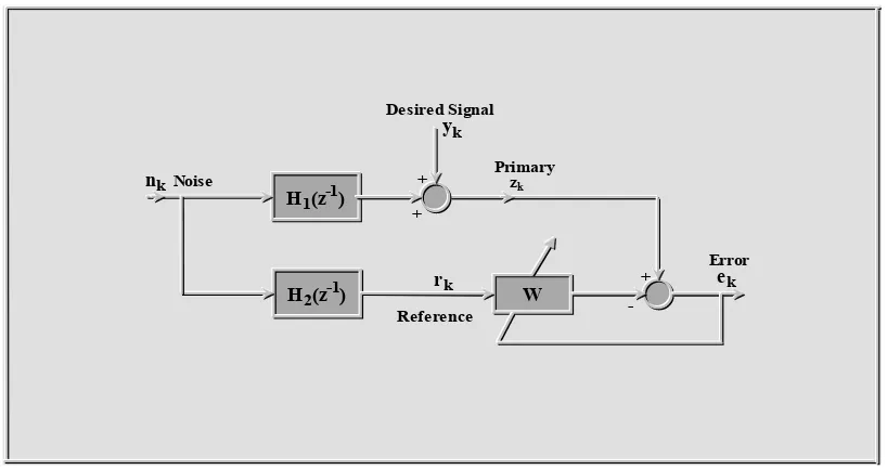
[1]. This approach illustrated in figure 1 uses two inputs, a primary input and a reference input.
+
W - ek
H1(z-1)
H2(z-1)
+
+
Primary
Reference
nkNoise
Error
yk
Desired Signal
zk
[image:1.595.132.541.398.615.2]rk
Figure 1 : Adaptive Noise Canceller
where the noise nk reaches both the primary and reference inputs via different acoustic transfer
functions H1(z-1) and H2(z-1) respectively. Here it is assumed that the desired signal is only
received at the primary input.
Although in practice this may not be the case, it is not central to the arguments in this paper. This noise cancelling method has been studied extensively and most of the properties are known
in the literature [2]. For example, the step size in the LMS algorithm µ must be chosen in such a
way that convergence (and hence tracking) is fast whilst at the same time ensuring that stability is maintained. This is particularly a problem when the noise data is non-stationary as an over
select µ as large as possible consistent with stability. The paper will show that even if µ is chosen to be well within the bounds of stability (for example, one tenth of its theoretical maximum) then a second problem occurs. Cross modulation terms of signal x noise are fed
through and appear as distortion on the final noise cancelled error output ek.
2 The LMS Algorithm
Consider the ordinary LMS algorithm applied to the noise cancellation problem of Figure 1.
e
ky
kX W
kT k 1=
−
− (1)W
k=
W
k 1−+
2 X e
µ
k k (2)where the weight vector
W
k=
[w w
o 1w ]
n T and Xk is the vector of regressors of rk givenby
X
k=
[r r
k k 1−r
k n−]
T, n is the order of the adaptive filter with (n+1) weights.Define the variance of rk as E[rk2] = σr2 where E[rk] = 0. Also define the correlation matrix R =
E[XkXTk]. Then the two well established formulae for convergence become [2].
Convergence in the mean:
µ
λ
≺
1
max(3)
where
λ
max is the largest eigenvalue of the correlation matrix R.Convergence is the mean square
(
)
µ
σ
≺
1
1
2n
+
r (4)By choosing the step size parameter µ to satisfy (4) convergence in the mean (equation (3)) is
automatically satisfied [2]. If equation (4) is used as an equality, the LMS algorithm will be
unstable. Usually µ is chosen to be at least one third of
1
1
2(
n
+
)
σ
r or even smaller values[3, 4]
Control System Approach
Kwong [5, 6] has used modern control theory to explain some important properties of LMS,
namely the effect of gradient noise and the optimum step size. Similarly, Dabis and Moir [7]
have examined the LMS algorithm using classical control theory. This work is extended in [8]
to give an expression for
µ
in terms of bandwidth.It has been shown that
(
)
µ
θ
σ
=
−
+
1
2
1
2cos
Br
n
(5)and phase margin ϕm
φ
π θ
θ
θ
m B B
B
= −
−
−
−tan
sin
cos
11
(6)where θB is the normalised bandwidth frequency in radians.
In [7, 8] the step size is analogous to a constant gain in a servo mechanism whilst φm defines the
stability. For example, for a maximum bandwidth
θ
B=
π
radians;
µ
=
1
(
n
+
1
)
σ
2r and
the phase margin is zero degrees indicating instability as expected. For a more conservative
72o, well within acceptable limits. The problem is further compounded by the fact that the gain within the closed loop system of the LMS algorithm is time varying. This is best illustrated with a block diagram. Suppose for simplicity that only one parameter is to be estimated.
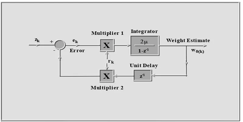
The block diagram for such a problem is shown in Figure 2.
+
- 1-z-1
z-1
Integrator
Unit Delay
w0(k)
Weight Estimate Multiplier 1
Multiplier 2
X
X
ek Error
2µ
rk
[image:3.595.144.543.169.369.2]zk
Figure 2 : Block diagram of LMS for one parameter
It can be seen that the block diagram consists of negative feedback around a discrete integrator
with gain µ. Two multipliers within the loop imply that the overall gain will vary from each
sampling instant. Since all signals and noise are zero mean, µ will define an average bandwidth
via equation (5). The unit delay z-1 in the feedback path ensures physical reliability of the
algorithm as a closed-loop discrete control system cannot respond instantaneously. If the discrete integrator and unit delay are replaced with a continuous time integrator, then the closed loop system can theoretically never be unstable. This property that the gain for continuous time
LMS has no upper bound has been noted by Karni and Zeng [9]. Both continuous and discrete
versions of LMS have the same limitations on bandwidth which is born out with the following simple examples.
3 Illustrative Examples
The following examples show that a much smaller value of step size is required than is
predicted by stability considerations. Whilst the algorithm will be stable, an unacceptable amount of distortion will be present.
Example 1
Consider a periodic signal with periodic noise. Define H1(z-1) = m (a constant) and H2(z-1) = 1.
Then rk = cos(θrk), yk = cos (θyk), zk = cos (θyk) + m cos (θrk)) where θr= 2πfr/fs and θy= 2πfy/fs
The frequencies fy, fr,fs are respectively the signal, noise and sampling frequencies.
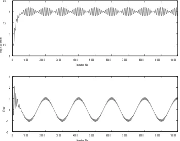
Taking m = 2, fs = 10kHz, fy = 5Hz, fr = 100Hz the LMS algorithm is examined with different µ
values.
The single weight to be estimated is wo = 2. Figures 3, 4 and 5 show this weight estimate and
the error output for three µ values obtained from equation (5). The three bandwidths chosen are
respectively as 1kHz, 100Hz and 10Hz.
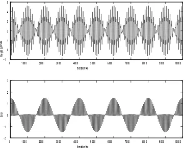
In Figure 3 it can be seen that the mean weight estimate is 2 but it fluctuates around this value.
To get an expression for the weight vector it is necessary to look at the input to the integrator uk
through unfiltered. For high bandwidth ek = cos (θyk) + m cos (θrk) and rk = cos (θrk). The
integrator input µk = ekrk which becomes
(
)
(
)
(
)
u
k
k
m
k
k
k
m
k
k y r r
y r r y
r
=
+
=
+
+
−
+
+
cos (
) cos (
)
cos (
)
cos (
)
cos (
)
cos
θ
θ
θ
θ
θ
θ θ
θ
21
2
1
2
2
1
2
(7)
Equation (7) describes a double sideband suppressed carrier waveform (DSSC), a DC term m/2
and a term at twice the reference frequency (200Hz). The DSSC spectrum is centred at 100Hz
with side bands at
±
5Hz. For a bandwidth of 1kHz (one tenth sampling frequency) all thefrequencies in (7) will pass unfiltered and this is what appears in Figure 3.
0 1000 2000 3000 4000 5000 6000 7000 8000 9000 10000 -1 0 1 2 3 4 5 Iteration No W eig ht Es tim ate
[image:4.595.94.457.313.607.2]0 1000 2000 3000 4000 5000 6000 7000 8000 9000 10000 -2 -1 0 1 2 3 Iteration No Er ro r
0 1000 2000 3000 4000 5000 6000 7000 8000 9000 10000 0
1 2 3 4
Iteration No
W
eig
ht
Es
tim
ate
0 1000 2000 3000 4000 5000 6000 7000 8000 9000 10000 -2
-1 0 1 2 3
Iteration No
Er
ro
[image:5.595.159.482.146.411.2]r
0 1000 2000 3000 4000 5000 6000 7000 8000 9000 10000 0
0.5 1 1.5
2 2.5
Iteration No
W
eig
ht
E
sti
m
at
e
0 1000 2000 3000 4000 5000 6000 7000 8000 9000 10000 -2
-1 0 1 2 3
Iteration No
Er
ro
r
Figure 5 Weight Estimate for 10Hz Bandwidth
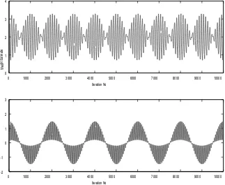
In Figure 4, the bandwidth drops to 100Hz and the term at 200Hz becomes filtered leaving DSSC as the weight estimate with a DC level. The error signal (signal estimate) is still severely distorted. Finally in Figure 5 when the bandwidth is 10Hz the error becomes the 5Hz signal and the weight becomes closer to 2. Since the bandwidth has been reduced by a decade the feed-through term has also been reduced by 20dB (single integrator dynamics). If the bandwidth is reduced further the noise can be almost entirely removed at the expense of slow adaptation. For this example the DSSC waveform will have a spectrum with upper sideband at 105Hz and lower sideband at 95Hz. Therefore by choosing the bandwidth of the LMS algorithm via (5) to be an order of magnitude less than 95Hz the DSSC is attenuated sufficiently. In phaselock loops
(PLL’s) a related problem exists where 2fc (fc is the carrier frequency) terms permeate onto the
demodulated baseband signal. In PLL’s the bandwidth is usually chosen to be (2fc/10). For
LMS by analogy it must be fL/10 where fL is the lowest sideband in the product of primary x
[image:6.595.94.449.148.426.2]Example 2
Consider a periodic signal at a frequency of 100 Hz with sampling frequency
10kHz. The noise is narrowband with bandwidth 40Hz centred also at 100Hz. The noise is generated by passing zero-mean white Guassian noise with unit variance through a fourth order discrete IIR Butterworth filter. The set-up is as shown in Figure 1 with the filter
( ) ( ) ( )
( )
H z
1B z
A z
H z
1 1 1
2 1
1
−
=
−/
−and
−=
. The polynomialsB(z-1) and A(z-1) were generated using MATLAB and are respectively
( )
( )
(
)
A z
z
z
z
z
z
z
z
z
B z
z
z
z
z
− − − − − − − − −
− − − − − −
= −
+
−
+
−
−
−
+
=
−
+
−
+
1 1 2 3 4 5 6 7 8
1 6 2 4 6 8
1 8
27 45
54 4
67 4
535
26 6
7 5
0 94
10
0 024 0 096
0145
0 096
0 024
.
.
.
.
.
.
.
.
.
.
.
.
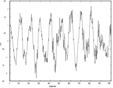
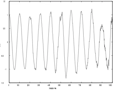
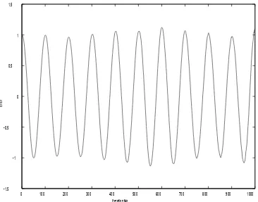
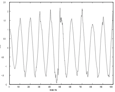
The adaptive filter was chosen to be order n = 20. Figures 6,7 and 8 show the error (the signal estimate) for bandwidths of 1kHz, 100Hz and 10Hz respectively.
0 100 200 300 400 500 600 700 800 900 1000 -2.5
-2 -1.5
-1 -0.5
0 0.5
1 1.5
2 2.5
Iteration No
Er
ro
[image:7.595.151.520.340.628.2]r
0 100 200 300 400 500 600 700 800 900 1000 -1.5
-1 -0.5
0 0.5
1 1.5
Iteration No
Er
ro
[image:8.595.97.459.146.435.2]r
0 100 200 300 400 500 600 700 800 900 1000 -1.5
-1 -0.5
0 0.5
1 1.5
Iteration No
Er
ro
[image:9.595.152.518.144.431.2]r
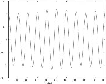
Figure 8 Signal Estimate for 10Hz Bandwidth
As expected the signal to noise ratio improves with a reduction in µ. In example 1, the
bandwidth of the LMS algorithm is reduced so as to significantly reduce the lowest sideband in the spectrum of the product of the primary x reference signals. Since in this case the reference signal is white noise, the product will have power across the spectrum. Only the DC content of this product is required by the integration of the LMS algorithm. By reducing the bandwidth sufficiently some feedthrough terms are attenuated at the expense of poor tracking. In order to achieve good cancellation (reduction in feedthrough terms) and high bandwidth a modification is
required. If the reference signal rk is filtered by a high pass filter up to say 2kHz, then there will
0 100 200 300 400 500 600 700 800 900 1000 -2
-1.5 -1 -0.5
0 0.5
1 1.5
2 2.5
Iteration No
Er
ro
[image:10.595.96.463.143.436.2]r
0 100 200 300 400 500 600 700 800 900 1000 -1.5
-1 -0.5
0 0.5
1 1.5
Iteration No
Er
ro
[image:11.595.154.517.146.433.2]r
Figure 10 Signal Bandwidth for 100Hz Bandwidth
Comparing Figures 6 and 9 show the improvement in highpass filtering the reference signal before applying it to the LMS algorithm. Figures 10 illustrates the near perfect recovery of the original waveform except for minor amplitude modulation.
5 Conclusions
It has been shown that there is advantage in considering the LMS algorithm as a control system as applied to noise cancellation.
If the spectrum of the primary and reference signals are known, a priori, (a practical proposition)
then the best strategy can be used to obtain maximum tracking ability and good filtering action.
It has been shown that cross modulation terms will feedthrough and cause distortion if µ is
chosen to be too large. Conversely, it is well established that for small µ the convergence will
be slow. To obtain the best value for µ the lowest sideband frequency in the spectrum of the
product primary x reference must be sufficiently attenuated. This sideband frequency defines the
nominal bandwidth of the LMS algorithm and hence µ via equation (5). When the reference is
wideband, it is possible to highpass filter it to attenuate frequencies below a defined bandwidth. The bandwidth will be as high as possible consistent with closed-loop stability. These methods give fast convergence and hence good tracking whilst maintaining good filtering action.
The results apply equally to continuous time LMS where stability is less of a problem than the
6 References
[1]B. Widrow and S.D. Stearns (1985) : Adaptive signal processing, Prentice Hall, Englewood
Cliffs, NJ.
[2] S. Haykin (1986) : Adaptive Filter Theory, Prentice Hall, Englewood Cliffs, NJ.
[3] A. Feuer and E. Weinstein, E. (1985) : Convergence Analysis of LMS filters with uncorrelated Guassian data, IEEE Trans. ASSP, Vol. 33, No. 1, pp 222-229.
[4]L.L. Horowitz and K. Senne, (1981) : Performance Advantage of Complex LMS for
Controlling Narrow-band Adaptive Arrays, IEEE Trans. ASSP, Vol. 29, No.3, pp 722 - 736.
[5]C.P. Kwong (1990) : Control-theoretic design of the LMS and the sign algorithm in
Nonstationary environments, IEEE Trans. ASSP, Vol. 38, No. 2, pp 253-259.
[6]C.P. Kwong (1993), Further results on the control-theoretic analysis of the LMS algorithm,
IEEE Trans, ASSP, Vol. 41, No.2, pp 943-946.
[7]H.S. Dabis and T.J. Moir (1991) : Least mean squares as a control system, Int. Jour Control,
Vol. 54, No.2, pp 321-335.
[8]T.J. Moir (1994 ) : The Application of servo theory to the LMS algorithm, Proc. EUSIPCO
‘94, Sept. 13-16, Edinburgh, Scotland, pp 1277-1280.
[9]S. Kami and G. Zeng (1989) : The Analysis of the Continuous-Time LMS algorithm, IEEE
Trans. ASSP, Vol. 37, No.4, pp 595-597