Parallel in space time, adaptive finite element framework for non linear parabolic equations

PARALLEL-IN-SPACE-TIME, ADAPTIVE FINITE ELEMENT

FRAMEWORK FOR NONLINEAR PARABOLIC EQUATIONS

∗

ROBERT DYJA†, BASKAR GANAPATHYSUBRAMANIAN‡, AND KRISTOFFER G. VAN DER ZEE§

Abstract. We present an adaptive methodology for the solution of (linear and) nonlinear time dependent problems that is especially tailored for massively parallel computations. The basic concept is to solve for large blocks of space-time unknowns instead of marching sequentially in time. The methodology is a combination of a computationally efficient implementation of a parallel-in-space-time finite element solver coupled with a posteriori space-parallel-in-space-time error estimates and a parallel mesh generator. While we focus on spatial adaptivity in this work, the methodology enables simultaneous adaptivity in both space and time domains. We explore this basic concept in the context of a variety of time steppers including Θ-schemes and backward difference formulas. We specifically illustrate this framework with applications involving time dependent linear, quasi-linear, and semilinear diffusion equations. We focus on investigating how the coupled space-time refinement indicators for this class of problems affect spatial adaptivity. Finally, we show good scaling behavior up to 150,000 proces-sors on the NCSA Blue Waters machine. This conceptually simple methodology enables scaling on next generation multicore machines by simultaneously solving for a large number of timesteps, and reducing computational overhead by locally refining spatial blocks that can track localized features. This methodology also opens up the possibility of efficiently incorporating adjoint equations for er-ror estimators and inverse design problems, since blocks of space-time are simultaneously solved and stored in memory.

Key words. parabolic problems, parallel-in-time, finite element method, adaptive mesh refine-ment

AMS subject classifications. 65M22, 65Y05

DOI. 10.1137/16M108985X

1. Introduction.

We describe the methodology and application examples of

space-time block adaptive solutions to parabolic partial differential equations. This

approach is primarily motivated by the necessity of designing computational

method-ologies that can scale to leverage the availability of very large computing clusters

(exascale and beyond). For evolution problems, the standard approach of

decom-posing the spatial domain is a powerful paradigm of parallelization. However, for

a fixed spatial discretization, the efficiency of purely spatial domain decomposition

degrades substantially beyond a threshold—usually tens of thousands of processors—

which make this approach unsuitable on larger machines.

1

_{To overcome this barrier,}

∗_{Submitted to the journal’s Software and High-Performance Computing section August 17, 2016;}

accepted for publication (in revised form) November 27, 2017; published electronically May 1, 2018. http://www.siam.org/journals/sisc/40-3/M108985.html

Funding: The work of the first and second authors was supported by NSF 1435587, NSF XSEDE resources at TACC, as well as an exploratory account on NCSA Blue Waters (with thanks to Brett Bode). The work of the third author was supported by the Engineering and Physical Sciences Research Council (EPSRC) under grant EP/I036427/1.

†_{Czestochowa University of Technology, 42-201 Czestochowa, Poland ([email protected]).} ‡_{Corresponding author. Iowa State University, Ames, IA 50011 ([email protected]).}

§_{School of Mathematical Sciences, University of Nottingham, University Park, Nottingham NG7}

2RD, UK ([email protected]).

1_{There are a few approaches that scale reasonably well even on very large number of processors;}

see, for instance, Dendro [29]. However, there is still a case to be made for space-time approaches; for example, moderate spatial problems that have to be solved over a long time horizon.

a natural approach is to consider the time domain as an additional dimension and

simultaneously solve for blocks of time, instead of the standard approach of sequential

time stepping [12].

This concept of solving for blocks of space-time has resulted in several promising

approaches to time parallel integration that have been developed over the past century,

but which are gaining increasing attention due to that availability of appropriate

com-puting resources. Broadly

2

one can consider three types of parallelization approaches

to solving a space-time problem. The first type of methods explicitly parallelizes only

over time, and leaves spatial parallelism (and spatial adaptivity) undefined [21, 12].

These methods may also be considered as shooting methods [15]. The second type

of methods explicitly parallelizes over space, and leaves temporal parallelism (and

temporal adaptivity) undefined. These methods include wave form relaxation

meth-ods that attempt to reconcile the solution at spatial boundaries between space-time

blocks [15]. The third type of methods explicitly targets parallelism (and adaptivity)

in space and time. The current work seeks to advance type three methods. In the

more narrow context of finite element methods, early work on type three methods

was considered by Hughes and coworkers [19, 18], Tezduyar et al. [30], and Potanza

and Reddy [26], while variations on this theme have recently been explored by several

groups [6, 8, 22, 23, 27, 34].

The concept of solving for blocks of time simultaneously has recently gained a lot

of attention to enable effective usage of exascale computing resources.

3

In addition to

this obvious advantage, solving for space-time blocks also allows natural incorporation

of a posteriori error estimates for mesh adaptivity, and enables the solution of inverse

problems involving adjoints [14, 13]. This has several additional tangible benefits

in the context of computational overhead. For evolution problems—including wave

equations, and problems involving moving interfaces like bubbles and shocks—that

exhibit localized behavior in space and time, solving in blocks of space-time that

are locally refined to match the local behavior provides substantial computational

gain [8]. Similarly, the availability of error estimates across a block of time allows

optimal choices of space and time adaptivity.

Motivated by these considerations, this paper presents a methodology for the

so-lution of time dependent linear, quasi-linear, and semi-linear diffusion equations in

three dimensions. We discuss the development of a parallel adaptive framework for

the solution of large blocks of space-time. We detail the development of the block

space-time framework for two classes of time steppers (

θ

-schemes, backward

differ-ence formula (BDF)). We subsequently define

a posteriori space-time error indicators

to identify spatial regions for mesh adaption. We show representative results

us-ing problems with analytical solutions and illustrate scalus-ing behavior up to 150,000

processors. Finally, we demonstrate that for sufficiently large problems the block

space-time approach enjoys a substantial speedup over sequential time stepping.

The outline of the rest of the paper is as follows: sections 2 and 3 detail the block

space-time framework for linear and nonlinear evolution equations, respectively.

Sec-tion 4 discusses the space-time error estimates for these classes of problems. In secSec-tion

5, we discuss implementation details. Section 6 illustrates several numerical

exam-ples of the framework and shows scaling performance and analysis. We conclude in

section 7.

2_{We thank the anonymous reviewer for suggesting this classification.}

3_{See, for instance, the U.S. DOE’s Exascale Mathematics Working Group [17].}

2. Basic space-time formulation: linear and nonlinear versions.

2.1. Space-time framework for a linear problem.

Given a bounded domain

Ω

∈

R

3

, and a finite time domain [0

, T

], consider the parabolic equation that solves,

for

u

: Ω

×

[0

, T

]

→

R

,

(1)

(

∂

t

u

(x

, t

)

− ∇ ·

κ

∇

u

(x

, t

) =

f

(x

, t

)

in Ω

×

[0

, T

]

,

u

(x

,

0) =

u

0

,

where

f

: Ω×[0

, T

]

→

R

is a smooth source function, and

κ >

0. We consider, without

loss of generality, that Dirichlet boundary conditions are imposed on the boundary Γ,

unless otherwise specified. Considering a tessellation,

T ≡ {Ω

1

_{, . . . ,}

_Ω

e

_{, . . .}

_{}, of the}

domain Ω into elements with average size

h

, the weak form of this equation is given

as

(2)

(

find

u

h

_(·

_{, t}

₎

_{∈ U}

h

_:

(

w

h

_{, ∂}

t

u

h

(·

, t

)) + (∇

w

h

, κ

∇

u

h

(·

, t

)) = (

w

h

, f

)

∀

w

h

∈ V

h

,

where (

. , .

) is the

L

2

inner product on Ω and

(3)

U

h

_:=

u

h

|

u

h

∈

H

1

(Ω)

,

u

h

∈

P

(Ω

e

)

∀

e

,

V

h

:=

w

h

|

w

h

∈

H

1

(Ω)

,

w

h

∈

P

(Ω

e

)

∀

e

with

P

(Ω

e

_{) being the space of the standard polynomial finite element shape}

func-tions on element Ω

e

_{. To obtain a fully discretized form, we employ a time-stepping}

technique on the above semidiscrete equation. While any time-stepping method can

be used, as an example, consider the Euler backward formula that is defined on a

discretization

{0

, t

1

, t

2

, . . . , T

}

of the time domain:

(4)

w

h

,

u

h n+1

−

u

hn

∆

t

+

∇

w

h

, κ

∇

u

h_n+1

=

w

h

, f

n+1

for

n

= 0

,

1

, . . . ,

where the subscript denotes evaluation at that discrete time, and ∆

t

=

t

n+1

−

t

n

is

the time step.

Following standard FEM practice, with the tessellation of the domain resulting

in

k

nodal values that describe spatial variation of the field

u

, (4) can be expressed

in terms of matrix-vector products as

(5)

Mu

n+1

+ ∆

t

Ku

n+1

=

Mu

n

+ ∆

t

f

n+1

for

n

= 0

,

1

, . . . ,

where

M

and

K

are the global mass and stiffness matrices, respectively.

4

_u

n+1

and

u

n

are vectors containing the nodal values of the field

u

at time step

n

+ 1 and

n

,

respectively. Equation (5) represents the system of equations solved to get the solution

for time step

n

+ 1. The size of vector

u

is equal to the number of nodal unknowns,

k

. Similarly matrices

K,

M

are sparse matrices of size

k

×

k

.

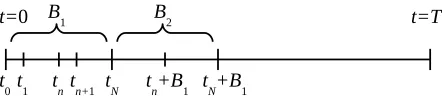
Consider a blockwise division of the total time domain. Each block,

B

i

, consists

of multiple time steps. This is schematically represented in Figure 1. Instead of

sequentially solving for each time step (as in (5)), consider solving for the field variable

in a complete time block,

B

, consisting of

N

time steps simultaneously, i.e., solve for

u

i

, i

= 1

, . . . , N

, simultaneously.

4_{With some abuse of notation, the elements of matrixMare equal toM}

ij= (whi, whj) and matrix

Kare equal toKij= (∇whi, κ∇wjh).

B

₁

B

₂

t=

0

t

_n

t

_n+1

t

_N

t

_N

+B

₁

t=T

t

₀

t

₁

t

_n

+B

₁

Fig. 1. Indexing of time steps per block(B). Number of time steps per block is equal to N.

This results in a block diagonal matrix of size (

N

×

k

)-by-(

N

×

k

) given by

(6)















I

−M

M

+ ∆

t

K

−M

M

+ ∆

t

K

. .

_.

−M

M

+ ∆

t

K





























u

0

u

1

u

2

..

.

u

N















=















IC

∆

t

f

1

∆

t

f

2

..

.

∆

t

f

N















,

where

I

is an identity matrix (of size

k

) and the IC are the imposed initial conditions.

This system solves for

N

time steps at once with a total number of unknowns equal

to

N

×

k

.

Remark

1. Essentially, we convert the problem of sequentially solving for N time

steps into a problem of solving for N unknowns simultaneously. By treating the

un-known nodal values at different time steps as multiple degrees of freedom (DOFs)

associated with each spatial node, we can leverage standard algorithmic approaches

(assembly, memory usage) tailored for multiple DOFs problems. Note that by framing

the temporal unknowns as multiple DOFs at each spatial point, the load distribution of

the problem across processors is still based on a distribution of the spatial mesh across

P

processors. However, each processor now has

N

times more unknowns than the

sequential case (5). This allows

P

to be much larger than for the sequential case while

allowing for efficient parallel performance.

5

_{Many approaches in uncertainty}

quantifi-cation (polynomial chaos representation, spectral stochastic methods) leverage such

an approach of representing field variation along additional dimensions (stochastic

dimensions) as simply an additional DOF at each spatial location [25, 33, 10, 28].

2.2. Space-time framework for nonlinear problems.

Extending the

ap-proach to certain nonlinear problems is straightforward. Consider the case where

κ

is a function of the dependent variable,

u

. We assume that

κ

(

u

) satisfies

appropri-ate smoothness and boundedness assumptions to ensure existence and uniqueness,

0

< κ

≤

κ

(

u

)

≤

κ <

∞. In this case the weak form for a block

B

is

(7)

w

h

,

u

h n+1

−

u

hn

∆

t

+

∇

w

h

, κ

(

u

h_n+1

)∇

u

h_n+1

=

w

h

, f

n+1

for

n

= 0

,

1

, . . . , N .

The solutions to such nonlinear equations are usually via (quasi-)Newton schemes.

The methodology involves construction of the Jacobian and residual, which are used

to compute updates. This is represented in matrix-vector terms as

J

_ui n+1

δ

u

i+1

n+1

=

F

ui n+1

,

u

i+1

n+1

=

u

i

n+1

+

δ

u

i+1

n+1

(8)

for

i

= 1

, . . . ,

until convergence and for

n

= 0

,

1

, . . . ,

5_{This is specifically illustrated in the results which show scalability for a range of differentN=}

1,10,50,100,200,500,1000.

[image:4.612.146.367.94.144.2]

where

J

_ui

n+1

is the Jacobian (or linearized form), and

F

uin+1

is the residual of the above

equation, both computed using

u

i

n+1

. More specifically, for the nonlinear diffusion

equations defined by (7), the residual,

F

_ui

n+1

, is given by

(9)

F

_ui n+1

=

1

∆

t

Mu

i n+1

−

1

∆

t

Mu

n

−

K(u

i n+1

)u

i

n+1

−

f

n+1

,

where

K(u

i

n+1

) denotes the solution dependent stiffness matrix. The Jacobian is given

as

(10)

J

ui n+1

=

1

∆

t

M

+

K(u

in+1

) +

dK(u

i

n+1

)

d

u

.

Instead of sequentially solving for each time step (as in (9)), consider solving for

the field variable in a complete time block,

B

, consisting of

N

time steps

simultane-ously. That is,

(11)











J

ui

1

−

1

∆t

M

J

ui

2

. .

_.

−

1

∆t

M

J

ui

N





















δ

u

i₁+1

δ

u

i₂+1

..

.

δ

u

i_N+1











=











F

ui

1

F

ui

2

..

.

F

_ui

N











and











u

i₁+1

u

i₂+1

..

.

u

i_N+1











=











u

i1

u

i2

..

.

u

i N











+











δ

u

i₁+1

δ

u

i₂+1

..

.

δ

u

i_N+1











.

Remark

2. One can alternatively ignore the off-diagonal entries of the block

Ja-cobian to construct an approximate diagonal JaJa-cobian.

The propagation of time

information is then limited to the residual on the right-hand side. We tried both

approaches, with the latter approach taking more iterations to convergence, while

providing substantial ease of implementation. Unless otherwise stated, all our results

are based on the latter approach.

3. Space-time formulation: Higher-order time schemes.

We next look at

extending the space-time strategy to incorporate two families of higher-order

time-steppers: Θ-scheme and BDF. We consider linear and nonlinear diffusion and,

more-over, we also consider the treatment of the Allen–Cahn equation, which is a parabolic

PDE with a lower-order nonlinearity, whose solution has evolving layers and for which

adaptivity is particularly useful.

3.1. Θ-scheme: Linear equation.

The semidiscrete form of the Θ-scheme—

which is a generalization of the Euler backward scheme—is as follows:

(12)

(

w, u

n+1

)

−

(

w, u

n

) + ∆

t

[(1

−

Θ) (∇

w, κ

∇

u

n

) + Θ (∇

w, κ

∇

u

n+1

)]

= ∆

t

[(1

−

Θ) (

w, f

n

) + Θ (

w, f

n+1

)] for

n

= 0

,

1

, . . . .

The fully discrete matrix-vector representation is given by

(13)

Mu

n+1

−

Mu

n

+ ∆

t

(1

−

Θ)

Ku

n

+ ∆

t

ΘKu

n+1

= ∆

t

(1

−

Θ)

f

n

+ ∆

t

Θf

n+1

for

n

= 0

,

1

, . . . .

Again, it is straightforward to group and simultaneously solve for

N

time steps

to-gether. The corresponding matrix form is expressed as

(14)















I

−M

+ ∆

t

(1

−

Θ)K

M

+ ∆

t

ΘK

−M

+ ∆

t

(1

−

Θ)K

M

+ ∆

t

ΘK

. .

_.

−M

+ ∆

t

(1

−

Θ)K

M

+ ∆

t

ΘK





























u

0

u

1

u

2

..

.

u

N















=















IC

∆

t

[(1

−

Θ)f

0

+ Θf

1

]

∆

t

[(1

−

Θ)f

1

+ Θf

2

]

..

.

∆

t

[(1

−

Θ)f

N−1

+ Θf

N

]















.

Again, the global space-time matrix (15) has a block structure.

3.2. Θ-scheme: Nonlinear diffusion with variable coefficient.

The

corre-sponding weak form for this case is given as

(15)

w

h

,

u

h n+1

−

u

hn

∆

t

+ (1

−

Θ)

∇

w

h

, κ

(

u

h_n

)∇

u

h_n

+ Θ

∇

w

h

, κ

(

u

h_n+1

)∇

u

h_n+1

= (1

−

Θ)

w

h

, f

n

+ Θ

w

h

, f

n+1

for

n

= 0

,

1

, . . . .

The Jacobian is

(16)

J

_ui

n+1

=

M

+ ∆

t

Θ

K(u

i_n+1

) +

dK(u

i n+1

)

d

u

,

while the residual is given by

(17)

F

ui

n+1

=

Mu

i

n+1

−Mu

n

+ ∆

t

Θ

K(u

in+1

)u

i

n+1

−

f

n+1

+ ∆

t

(1

−

Θ) (K(u

n

)u

n

−

f

n

)

.

Again, it is straightforward to group and simultaneously solve for

N

time steps

to-gether. Define diagonal blocks equal to

(18)

D

k

=

M

+ ∆

t

Θ

K(u

ik

) +

d

K(u

i

k

)

du

with the the upper index denoting, as before, Newton–Raphson iteration. The

corre-sponding (diagonal) block Jacobian (see Remark 2) is given by

(19)











D

1

D

2

. .

_.

D

N











.

3.3. Θ-scheme: Allen–Cahn equation.

The Allen–Cahn equation is a

semi-linear diffusion equation with a nonsemi-linear reaction term:

(20)

∂

t

u

(x

, t

)

−

∆

u

(x

, t

) +

−2

f

(

u

) = 0

,

where

f

(

u

) is a nonlinear function of

u

, usually

f

(

u

) =

u u

2

₋

₁

. The initial

condi-tion is

u

(x

,

0) =

u

0

along with zero flux conditions in the boundaries.

The corresponding semidiscrete form is given as

(21)

w

h

, ∂

t

u

h

+

∇

w

h

,

∇

u

h

+

−2

w

h

, f

(

u

h

)

= 0

.

Using the Θ-scheme results in the fully discrete form

(22)

w

h

, u

hn+1

+ ∆

t

Θ

∇

w

h

,

∇

u

hn+1

+

−2

w

h

, f

(

u

hn+1

)

=

w

h

, u

h_n

−

∆

t

(1

−

Θ)

∇

w

h

,

∇

u

h_n

+

−2

w

h

, f

(

u

h_n

)

.

Again, it is straightforward to group and simultaneously solve for

N

time steps

to-gether. The corresponding (diagonal) block Jacobian is given as

(23)

















M

+ ∆

t

Θ

K(u

i

1

) +

−2 d

f(ui₁)

du

M

+ ∆

t

Θ

K(u

i

2

) +

−2 d

f(ui

2)

du

. .

_.

M

+ ∆

t

Θ

K(u

i_N

) +

−2 df(uiN)

du

















.

Alternative schemes for the Allen–Cahn equation and other phase-field models are

described in, e.g., [16].

3.4. BDF-based time steppers.

BDF-based time steppers of order

s

utilize

the solution at

s

previous time steps to construct the solution at the next time step.

A general

s

order BDF scheme is given as

(24)

s

X

k=0

α

k

u

n+k

= ∆

tβg

n+s

,

where the left-hand side is the BDF scheme representation of the time derivative,

∂u_∂t

,

in terms of the solution

u

i

at time point

i

, and the right-hand side collects all other

terms. Here,

α

and

β

are known BDF coefficients [7]. A first-order (

s

= 1) BDF

scheme is identical to the Euler backward scheme described earlier. The simplest

multistep scheme is for

s

= 2 and for the linear diffusion equation it is given as

(25)

w

h

, u

h_n+2

−

4

3

w

h

_{, u}

h n+1

+

1

3

w

h

_{, u}

h n

+

2

3

∆

t

∇

w

h

_{, κ}

_∇

_u

h n+2

=

2

3

∆

t w

h

_{, f}

n+2

.

Again, it is straightforward to group and simultaneously solve for

N

time steps

to-gether.

6

_{The corresponding space-time block equations are as follows:}

(26)















I

−M

M

+ ∆

t

K

1

3

M

−

4

3

M

M

+

2

3

∆

t

K

. .

_.

1

3

M

−

4

3

M

M

+

2

3

∆

t

K





























u

0

u

1

u

2

..

.

u

N















=















IC

∆

t

f

1 2

3

∆

t

f

2

..

.

2

3

∆

t

f

N















.

As expected, higher-order multistep methods produce block matrices that have a

larger bandwidth. It is clear that nonlinear problems can be treated similarly.

6_{Note that the first time step is approximated using a backward Euler time stepper as the}

second-order BDF scheme requires knowledge of the solution at two previous time steps.

4. Adaptive meshing for the block space-time method: Residual-based

error estimator.

A central idea of this work is to develop a block space-time

method-ology that can be integrated with mesh adaptivity. This will enable targeted

refine-ment of regions that exhibit variations in the corresponding block of time. Mesh

adaptivity requires the definition of an indicator function that determines which

re-gions of the space require refinement/coarsening. In this work, we build on prior work

and utilize standard residual-based error indicators (see, e.g., [4, 32, 31]) and construct

space-time analogues by averaging or taking the maximum across the time block.

Al-ternative duality-based indicators for nonlinear parabolic problems are described in,

e.g., [8, 9, 11].

Residual-based error indicators

η

e

are constructed for each spatial element, Ω

e

,

and consist of two terms—an interior residual,

r

int

and a jump residual,

r

jump

[32]:

(27)

η

_e2

=

h

2_e

k

r

h_int

k

2

L2_(Ω

e)

+

h

e

k

r

h jump

k

2

L2_(∂Ω

e)

,

where

h

e

is the size of element, Ω

e

. For example, for the linear and quasi-linear

diffusion equation, the detailed derivation of the interior and jump residual is available

in the work of Verf¨

urth [32]. We refer the interested reader to that work and only

show the key results here. Basically, the two terms are constructed (as the name

suggests) from the definition of the residual:

(28)

R

h

₍

_w

_{) = (}

_{w, f}

₎

₋

_{w, ∂}

t

u

h

− ∇

w, κ

(

u

h

)∇

u

h

.

This residual is decomposed into elementwise terms as

(29)

R

h

(

w

) =

X

e

Z

Ωe

wr

_inth

dΩ +

Z

Γe

wr

h_jump

dΓ

,

where

(30)

r

h_int

=

f

−

∂

t

u

h

+

∇ ·

κ

(

u

h

)∇

u

h

and

(31)

r

jumph

=

0

on

∂

Ω

e

∩

Γ

h

,

κ

(

u

h

)∇

u

h+

·

n

+

+

κ

(

u

h

)∇

u

h−

·

n

−

on

∂

Ω

e

\

Γ

h

,

where Γ

h

is that part of the boundary with Dirichlet conditions imposed.

The interior and jump residuals for the Allen–Cahn equations are similarly defined

as

(32)

r

h_int

=

−2

f

(

u

h

)

−

∂

t

u

h

+ ∆

u

h

and

(33)

r

h_jump

=

0

on

∂

Ω

e

∩

Γ

h

,

∇

u

h

+

·

n

+

+

∇

u

h−

·

n

−

on

∂

Ω

e

\

Γ

h

.

Recall that we are using error indicators defined over a block of time. We extend

the concept of error indicator defined at one time step to the notion of an error

indi-cator defined over a block of time steps. There are several choices of error indiindi-cators

with two of them being the average value of the error indicator across the block of

time for an element

e

,

(34)

η

e,avg

=

N

X

n=1

η

e,n

N

,

and the maximum value in the block of time for an element

e

,

(35)

η

e,max

=

max

n=1,2,...,N

η

e,n

.

The former approach is advantageous for slow variations in the block and avoids

frequent migrating of elements between processors, which can negatively affect

scal-ability. The latter approach is advantageous when there are rapid changes across a

few time steps. In this case the error estimator is not “diffused” by time steps where

the solution is changing slowly.

Remark

3. In this work, we approximate the semidiscrete term,

∂u

∂t

, in terms of

its finite difference representation (Θ or BDF scheme). An implicit assumption is that

the time steps are small enough that this approximation is valid. Ideally, one would

choose a consistent representation in both space and time, i.e., using a finite element

representation for time variations [26, 19]. This provides several advantages in terms

of mathematical elegance. We defer this development to a subsequent paper.

5. Implementation details.

We utilize our in-house scalable, parallel finite

ele-ment method (FEM) framework that is optimized for distributed memory computing.

The FEM software library is implemented in C++ and uses object oriented software

principles. Linear algebra, parallel matrix, and vector storage are all performed by

the PETSc library [5]. PETSc modules (KSP, SNES) are used to solve (non)linear

equations. Specifically, we use the hierarchical GMRES solvers as part of the PETSc

software suite (KSP construct) for solving the linear system. These solvers have been

shown to scale exceptionally well to hundreds of thousands of processors [24]. We use

the block Jacobi preconditioner in conjunction with the GMRES routine. The FEM

library is dynamically linked to the parallel hierarchical grid (PHG) library [2] which

is a three dimensional (3D) parallel mesh refinement framework with inbuilt load

bal-ancing. PHG uses a bisection-type algorithm [35], specifically newest vertex bisection

to refine/coarsen elements.

7

_{PHG operates on simplex elements and produces}

con-forming meshes after refinement. We remind the reader that we are able to utilize

parallel tools for 3D mesh adaptivity due to formulating our space-time problem as

a spatial problem with

N

DOFs. Additional implementation details are provided in

the appendix.

We perform scaling studies on two machines. Preliminary scaling was performed

on the TACC Stampede [3]. Stampede consists of 6400 compute nodes each equipped

with two Intel E5-2680 8-core processors. We also performed scaling on NCSA Blue

Waters [1]. Blue Waters consists of 22,640 nodes, each consisting of two AMD 6276

Interlagos processors for a total of 362,240 computing cores.

6. Numerical examples.

In this section we illustrate our adaptive

parallel-in-space-time framework on a variety of linear and nonlinear diffusion equations. We

show how the framework scales with increasing DOFs as well as increasing the size of

the time-blocks, i.e., increasing

N

.

6.1. Problem A: Linear diffusion.

We first consider the linear case.

We

set

κ

= 1 in (1), and consider a time horizon of

T

= 1. We use the method of

manufactured solutions to construct the forcing term in (1) to ensure an analytical

solution,

u

:

(36)

u

(

x, y, z, t

) = exp (−

α

(

x, y, z, t

))

,

7_{In the newest vertex bisection, the edge that lies opposite to the newest node is divided.}

where

α

(

x, y, z, t

) is equal to

(37)

α

(

x, y, z, t

) =

(

x

−

x

0

(

t

))

2

+ (

y

−

y

0

(

t

))

2

+ (

z

−

z

0

(

t

))

2

d

2

and

x

0

(

t

) =

a

cos(

ωt

) +

b ,

y

0

(

t

) =

a

sin(

ωt

) +

b ,

z

0

(

t

) =

b

with

a

= 0

.

2,

b

= 0

.

5,

ω

= 2

π

,

d

= 0

.

1. Thus,

u

is a rotating exponential hill centered

at the midplane and rotating on a circle with a radius of 0.2 and with an angular

speed of 2

π

(and hence a period of 1). This manufactured solution is constructed by

the following forcing term

(38)

f

(x

, t

) =

−

₄₍₍

_x

₋

_x

0

)

2

+ (

y

−

y

0

)

2

+ (

z

−

z

0

)

2

)

d

4

−

6

d

2

−

2

aω

cos(

tω

)(

y

−

y

0

)

−

sin(

tω

)(

x

−

x

0

)

d

2

exp (−

α

(

x, y, z, t

))

.

The equation is solved in the unit cube [0

,

1]

×

[0

,

1]

×

[0

,

1]. Every boundary face of

the region has an essential boundary condition with prescribed value of

u

equal to the

value computed from (36).

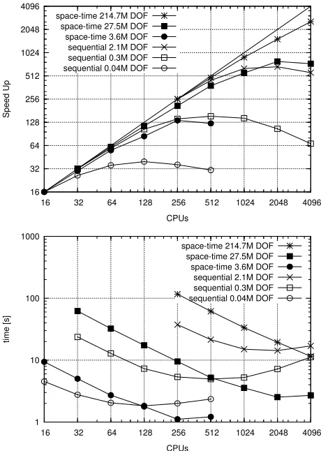
We first investigate the comparative scaling performance of the space-time

ap-proach with a sequential apap-proach. We use a time step of 0.01 and solve for a block

of 100 time steps. The space-time approach solves for this block of 100 time steps

simultaneously, while the sequential approach steps through the time steps, solving

for one time step at a time. Figure 2(top) shows scaling

8

_{on TACC Stampede for}

three sets of spatial discretization, 32

3

_{, 64}

3

_{, and 128}

3

_{trilinear elements. While this}

corresponds to 0

.

04

M,

0

.

3

M,

and 2

.

1

M

DOFs for the sequential approach (that is

then solved 100 times), the space-time approach corresponds to 3

.

6

M,

27

.

5

M

, and

214

.

7

M

DOFs (since they solve for all 100 time steps simultaneously). We can clearly

see that the space-time approach exhibits better scalability over a larger range of

processor counts, with the sequential approach tapering off at a much lower processor

count. For instance, for the 128

3

discretization, the space-time approach shows good

scaling behavior across the full range of processors investigated, while the sequential

approach exhibits its best performance at 1024 processors.

We next look at the

total time to solve

for the full time horizon [0

, T

]. We plot

this in Figure 2(bottom). As anticipated from the scaling studies, the space-time

approach gives consistent performance improvements for a larger range of processor

counts. This translates into consistent reduction of total time to solve with increasing

processor count. While the sequential approach has lower total time to solve for

smaller processor counts, beyond a certain processor count threshold the space-time

approach outperforms the sequential approach.

9

_{This is about 2048 processors for the}

largest spatial discretization (128

3

_{) considered. This bodes well for making a total}

8_{The minimum number of processors used for any problem in this work was 16. Thus all scaling}

results are compared with the 16 processor result.

9_{One of the reviewers pointed out that Figures 2(bottom) and 5(bottom) that explore strong}

scaling are similar to those produced by the parareal [21] (Lions, Maday, and Turinici) and multigrid reduction in time [12] (Falgout et al.) methods. It is interesting to see qualitatively similar results using different approaches to parallel-in-time.

16 32 64 128 256 512 1024 2048 4096

16 32 64 128 256 512 1024 2048 4096

Speed Up

CPUs space-time 214.7M DOF

space-time 27.5M DOF space-time 3.6M DOF sequential 2.1M DOF sequential 0.3M DOF sequential 0.04M DOF

1 10 100 1000

16 32 64 128 256 512 1024 2048 4096

time [s]

CPUs

space-time 214.7M DOF space-time 27.5M DOF space-time 3.6M DOF sequential 2.1M DOF sequential 0.3M DOF sequential 0.04M DOF

Fig. 2. Scaling studies on TACC Stampede. Comparison between sequential time stepping and the space-time approach. The equation being solved is the linear diffusion equation withN= 100time steps in a time block and discretized using the Euler backward scheme. The spatial discretizations used are323_,643_{, and128}3_{. Top plot shows speedup comparisons while bottom plot shows time to} solution.

time to solve argument when using large processor counts (especially, as will be shown

later in this section, using

∼

100,000 processors on the NCSA Blue Waters machine).

Furthermore, the total time to solve metric for the space-time approach will become

even more competitive for more complex problems involving complex geometries and

multiple remeshing that will require I/O.

Remark

4. In some sense, by solving problems in space-time instead of marching

forward in time, we are essentially making a computationally cheaper problem (of

solving a spatial problem at one time step) more expensive. However, as we make the

case,

10

_{there are several mitigating factors that warrant this approach. These factors}

include (a) hitting the limits of scaling when using purely sequential approaches, (b)

the ability to store and solve the full time horizon with significant implications to

solving adjoint problems, (c) the ability to only perform spatial adaptivity in blocks

greatly simplifying storage, and, finally, (d) as a first step to simultaneous adaptivity

in space and in time [19], which would prove very significant.

10_{Several other researchers have also made this case [12, 6, 20].}

[image:11.612.141.371.99.422.2]

32 64 128 256 512 1024 2048

32 64 128 256 512 1024 2048

Speed Up

CPUs sequential time stepper

10 time steps in block 50 time steps in block 100 time steps in block 200 time steps in block 500 time steps in block 1000 time steps in block

1 10 100 1000 10000

32 64 128 256 512 1024 2048

time [s]

CPUs

sequential time stepper 10 time steps in block 50 time steps in block 100 time steps in block 200 time steps in block 500 time steps in block 1000 time steps in block

Fig. 3. Speedup results on TACC Stampede for different sizes ofN. The equation being solved is the linear diffusion equation withN= 1,10,50,100,200,500,1000time steps in a time block and discretized using the Euler backward scheme. The spatial discretization is643_.

We next look at how increasing the number of time steps,

N

, in a time block

impacts performance of the space-time approach. Increasing

N

essentially increases

the DOFs per spatial node in the space-time framework. We again consider the time

interval [0

, T

= 1]. We investigate scaling behavior for a wide range of

N

ranging from

N

= 1 (the sequential case) to

N

= 1000. Figure 3(top) plots the scaling results on

TACC Stampede using up to 2048 processors. Notice that as

N

increases the curves

tend towards the ideal scaling line. This is consistent with earlier results in Figure

2 that show that increasing total DOFs results in better scaling performance. This

is especially encouraging as it indicates that utilizing larger blocks of time (which

translates to large total DOFs) results in lower total time to solve compared to a

sequential approach. This is clearly seen in Figure 3(bottom) which plots the total

time to solve over the full horizon [0

, T

]. The processor count at which the space-time

approach beats the sequential approach shows an increasing trend with increasing

N

,

with

N

= 10 taking less time than the sequential approach beyond just 256 processors,

and the

N

≥

200 potentially required more than 4096 processors to take less time

than the sequential approach.

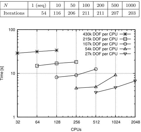
We next explore the number of GMRES iterations required to reach a relative

tolerance (−

ksp rtol

) of 10

−8

_{as a function of increasing}

_N

_{. Table 1 lists the number}

of iterations of the GMRES solver taken for various

N

’s with a spatial discretization

into 64

3

_{trilinear elements when run on 64 processors. Interestingly, the number of}

iterations saturates around 200 for

N

≥

50. We emphasize that we have not tried to

[image:13.612.138.378.131.356.2]

Table 1

Number of GMRES iterations needed to solve one space-time block of given size. In all cases the block Jacobi preconditioner was used. The spatial discretization is643_.

N 1 (seq) 10 50 100 200 500 1000

Iterations 54 116 206 211 211 207 203

1 10 100

32 64 128 256 512 1024 2048

Time [s]

CPUs

430k DOF per CPU 215k DOF per CPU 107k DOF per CPU 54k DOF per CPU 27k DOF per CPU

Fig. 4. Weak scalability results on TACC Stampede for different numbers of DOFs per CPU.

The same DOFs per CPU was achieved by using different numbers of time steps per block.

optimize the linear algebra portion (solver + preconditioner) of the method, relying

completely on PETSc modules. We expect that performance improvement may be

achieved by carefully choosing the solver and preconditioners as well as including the

full Jacobian (see Remark 2). An alternative question that we were unable to explore

in this work was to understand how the number of GMRES iterations changes as the

space-time system (and not just the time block,

N

) is refined.

While Figures 2 and 3 illustrate the

strong scalability

of the space-time approach,

we also test the

weak scalability

of the space-time framework. We consider five

dif-ferent starting problem sizes (i.e., a starting spatial discretization and

N

), which are

represented in terms of different DOFs per processor (

DOF s_proc

= 27

K,

54

K,

107

K,

215

K,

430

K

). For each starting problem size, we consider two doublings of the total DOFs

while keeping the DOFs per processor fixed (i.e., double the total problem size, but

also double the number of processors the problem is solved on). Figure 4 plots these

weak scalability results. Ideal weak scalability is said to be exhibited when the

to-tal time to solution remains unchanged with increasing toto-tal problem size. Here,

we see that for low DOFs per processor (27

K

, and 54

K

DOFs per processor) weak

scaling is quite poor, but improves significantly for higher DOFs per processor

sce-narios.

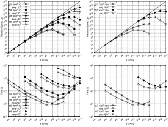
Having established that the space-time approach is well suited for deploying on

larger numbers of processors, we next look at scaling performance on the NCSA Blue

Waters machine. The NCSA Blue Waters machine allowed us to test the space-time

framework for a wide range of processor counts ranging from 2

4

_{= 32 processors up}

to 2

17

_{= 131}

_,

_{072 processors. We evaluate strong scaling under two campaigns of}

simulations. The first campaign considers

N

= 10, and four spatial discretizations

24

25

26

27

28

29

210

211

212

213

214

215

216

217

24 ₂5 ₂6 ₂7 ₂8 ₂9 ₂10 ₂11 ₂12 ₂13 ₂14 ₂15 ₂16 ₂17

Relative Speed Up

# CPUs ST 1003_*10

seq 1003

ST 2003_*10

seq 2003

HT 4003_*10

seq 4003

HT 8003_*10

seq 8003

24

25

26

27

28

29

210

211

212

213

214

215

216

217

24 ₂5 ₂6 ₂7 ₂8 ₂9 ₂10 ₂11 ₂12 ₂13 ₂14 ₂15 ₂16 ₂17

Relative Speed Up

# CPUs

ST 1003_*100

seq 1003

HT 4003_*100

seq 4003

10-1

100

101

102

103

24 ₂5 ₂6 ₂7 ₂8 ₂9 ₂10 ₂11 ₂12 ₂13 ₂14 ₂15 ₂16 ₂17

Time [s]

# CPUs

ST 1003_*10

seq 1003

ST 2003_*10

seq 2003

HT 4003_*10

seq 4003

HT 8003_*10

seq 8003

100

101

102

103

104

24 ₂5 ₂6 ₂7 ₂8 ₂9 ₂10 ₂11 ₂12 ₂13 ₂14 ₂15 ₂16 ₂17

Time [s]

# CPUs ST 1003_*100

seq 1003

HT 4003_*100

seq 4003

Fig. 5. Speedup on NCSA Blue Waters for linear diffusion equation with time blockN = 10

on the left andN= 100 on the right.

of the domain into 100

3

_{, 200}

3

_{, 400}

3

_{, and 800}

3

_{trilinear elements. The results of the}

scaling studies are plotted in Figure 5(left top). The space-time approach produces

consistent performance across a wide range of processors, with some degradation of

performance at very high processor counts. Figure 5(left bottom) plots the total

time to solve of the full time horizon [0

, T

] for this set of simulations. This plot

clearly shows that there is a processor count (especially for the larger problems 200

3

_,

400

3

_{, and 800}

3

_{) beyond which the space-time approach outperforms the sequential}

approach. These trends in scalability as well as the time to solve are even more

apparent in the second campaign that considers a larger time block of

N

= 100 (i.e.,

more DOFs per processor) and spatial discretizations of the domain into 100

3

_and

400

3

trilinear elements. The scalability results are plotted in Figure 5(right top), and

total time to solve results are plotted in Figure 5(right bottom).

We next look at the effect of adaptive meshing on the solution. Note that the

analytical solution to the PDE is a rotating exponential hill centered at the midplane.

We deploy the space-time approach with a residual-based error estimator considering a

time horizon of [0

, T

= 1] using a time step of 0.01. We consider a time block consisting

of

N

= 100, which is one full rotation of the exponential hill in the midplane. Figure 6

shows part of the refined spatial mesh after 20 refinement iterations. We remind the

reader that each iteration consists of solving the space-time problem, constructing the

time-averaged elemental refinement indicators using (34), and then refining the 3D

mesh according to the indicators. Given that this is a moving source problem, this

refinement is clearly around the location where the peak of the hill passes (centered

0.2 away from the midpoint with a thickness of 0.1).

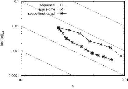
We finally compare spatial convergence rates for three implementations: (a)

se-quential time stepping with no spatial adaptivity, (b) space-time implementation with

[image:14.612.90.421.99.349.2]

Fig. 6.Refined mesh: view from top (left) and front (right).

0.0001 0.001 0.01 0.1

[image:15.612.143.382.99.211.2] [image:15.612.151.361.250.397.2]

0.01 0.1

last ||e||

L2

h sequential space-time space-time, adapt

Fig. 7.Spatial convergence for linear diffusion equation with time-step0.01. Error isku−uhk2 at the last time-step plotted as a function of the average element size¯h.

no spatial adaptivity, and (c) space-time implementation with spatial adaptivity. We

plot convergence in Figure 7, where the error is

k

u

−

u

h

k

2

. The first two

implementa-tions (obviously) overlap, with the adaptive mesh implementation showing a reduced

error. All three curves show a slope of 2, which is to be expected. Figure 8 shows

time-step convergence, with expected slopes of 1 and 2 for backward Euler and BDFs,

respectively.

6.2. Problem B: Nonlinear diffusion.

For the nonlinear case, we set the

coefficient

κ

(

u

) = 1 + 10

u

2

_{and we choose an exact solution such that}

_|

_u

_{| ≤}

_{1, thus}

bounding

κ

. As before, we choose our analytical solution to be given by (36). The

forcing term,

f

, is consequently

(39)

f

(x

, t

)

=

80

u

d

4

(

x

−

x

0

)

2

+ (

y

−

y

0

)

2

+ (

z

−

z

0

)

2

exp (−2

α

(

x, y, z, t

))

+ 1 + 10

u

2





4

(

x

−

x

0

)

2

+ (

y

−

y

0

)

2

+ (

z

−

z

0

)

2

d

4

−

6

d

2





exp (−

α

(

x, y, z, t

))

−

2

aω

cos(

tω

) (

y

−

y

0

)

−

sin(

tω

) (

x

−

x

0

)

d

2

exp (−

α

(

x, y, z, t

))

.

1e-05 0.0001 0.001 0.01

0.001 0.01

[image:16.612.150.362.100.246.2] [image:16.612.152.359.295.442.2]

0.1 1

last ||e||

L2

dt

EB BDF2

Fig. 8.Time convergence for linear diffusion equation. Error isku−uhk2at the last time step plotted versus time step.

24

25

26

27

28

29

210

211

212

213

214

215

216

217

24 ₂5 ₂6 ₂7 ₂8 ₂9 ₂10 ₂11 ₂12 ₂13 ₂14 ₂15 ₂16 ₂17

Relative Spe

ed Up

# CPUs

1003_*10

2003_*10

4003_*10

5503_*10

Fig. 9.Speedup on NCSA Blue Waters for the nonlinear diffusion equation.

The spatial and temporal domain over which the problem is solved remain

un-changed from the linear case. Similarly to the linear case, we investigate scaling

performance of the space-time approach. We however limit scaling studies to the

NCSA Blue Waters machine, which provides a larger range of processor counts. We

set

N

= 10, and consider four different spatial discretizations, 100

3

, 200

3

, 400

3

, and

550

3

. Figure 9 plots the scaling behavior of these problems across a wide range of

processor counts.

11

As before, the space-time approach exhibits very promising and

consistent scaling. While we do not show total time to solve analysis, our results

in-dicate that comparison with the sequential time-stepping approach will show similar

trends here as was shown for the case of the linear problem in Figure 5(left bottom).

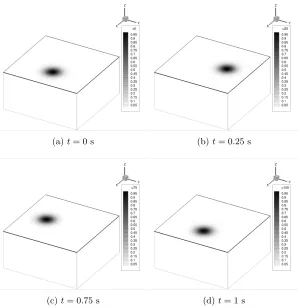
We next look at the effect of adaptive meshing on the solution. We deploy the

space-time approach with residual based error estimator for a time horizon of [0

, T

= 1]

using a time step of 0.01. We consider a time block consisting of

N

= 100, which

is one full rotation of the exponential hill in the midplane. Figure 10 plots several

time snapshots of the moving nonlinear source problem, with the solution accurately

11_{We use the PETSc SNES construct with a line search option. We set−ksp rtoland−snes rtol}

to 10−8_{for all runs.}

(a)t= 0 s (b)t= 0.25 s

[image:17.612.108.406.97.405.2]

(c)t= 0.75 s (d)t= 1 s

Fig. 10.Snapshots of the solution at different time points on the midplane.

0.0001 0.001 0.01 0.1

[image:17.612.151.360.456.601.2]

0.01 0.1

last ||e||

L2

h

sequential space-time, adapt space-time

Fig. 11.Spatial convergence for nonlinear heat equation with timestep0.01. Error isku−uhk2 at the last time step plotted as a function of the average element size¯h.

tracking the moving source. In Figure 11, we plot spatial convergence for three

im-plementations: (a) sequential time stepping with no spatial adaptivity, (b) space-time

implementation with no spatial adaptivity, and (c) space-time implementation with

24

25

26

27

28

29

210

211

212

213

214

215

216

217

24 ₂5 ₂6 ₂7 ₂8 ₂9 ₂10 ₂11 ₂12 ₂13 ₂14 ₂15 ₂16 ₂17

Relative Spe

ed Up

# CPUs

1003_*10

2003_*10

4003_*10

5503_*10

Fig. 12.Speedup on NCSA Blue Waters for Allen–Cahn problem.

spatial adaptivity (plotted with the average element size). Convergence rates follow

along expected lines with a slope of 2.

6.3. Problem C: Allen–Cahn.

In this final example, we solve the modified

Allen–Cahn problem. The key physics which is described by this nonlinear equation

essentially occurs in a highly localized region of the domain on a surface of codimension

1 which is evolving in time, thus representing a moving interface. Adaptive refinement

and coarsening has been a very effective approach to accurately resolve this localized

region, and a space-time approach with spatial adaptivity represents a very interesting

approach to solving this problem. The equation is given as

∂u_∂t

=

−

D f

(

u

)

−

C

n2

∇

2

u

,

where

(40)

f

(

u

) = 2

Au

1

−

3

u

+ 2

u

2

−

k

and

D

= 1,

C

n

= 0

.

1,

A

= 16,

k

= 0

.

1. The initial conditions are

(41)

u

(

x

) = 0

.

5 + 0

.

5 tanh





r

−

0

.

5

q

2

A

C

n





,

r

=

p

x

2

₊

_y

2

₊

_z

2

_,

with zero flux conditions on all boundaries. This represents an initial solid of radius,

r

= 0

.

5, that is melting. Using symmetry arguments, we consider a single octant of

the space [0 : 1]

×

[0 : 1]

×

[0 : 1]. Similarly to the previous cases, we investigate

scaling performance of the space-time approach. We again limit scaling studies to

the NCSA Blue Waters machine, which provides a larger range of processor counts.

We set

N

= 10 and use a time step of

δt

= 0

.

02, and consider four different spatial

discretizations of 100

3

_{, 200}

3

_{, 400}

3

_{, and 550}

3

_{trilinear elements. Figure 12 plots the}

scaling behavior of these problems across a wide range of processor counts. As before,

the space-time approach exhibits very promising and consistent scaling.

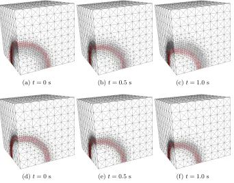
As a final result, we compare the adaptive mesh generated by the space-time

framework with the adaptive mesh generated by the sequential approach. We consider

the time domain [0

,

1] during which the initial sphere shrinks to about 70% of its

original volume. We choose a time step of

δt

= 0

.

02 and consider

N

= 50. We remind

the reader that each iteration consists of solving the space-time problem, constructing

the time-averaged elemental refinement indicators using (34), and then refining the

(a)t= 0 s (b)t= 0.5 s (c)t= 1.0 s

[image:19.612.89.431.96.363.2]

(d)t= 0 s (e)t= 0.5 s (f)t= 1.0 s

Fig. 13. Mesh after20refinement iterations with superimposed solution at times 0 s, 0.5s,

1s using the space-time adaptive approach (top). For comparison, view of adaptive mesh from the sequential solution (bottom).

3D mesh according to the indicators. In contrast, the sequential problem consists of

solving for each time step, constructing the refinement indicators, and then refining

the 3D mesh according to the indicators at each time step.

12

_{Figure 13 illustrates}

the adaptive mesh refinement across the time block with the top row representing

the space-time approach mesh and solution, and the bottom row representing the

sequential approach mesh and solution. Notice that in the sequential approach the

band of refined elements is moving with the moving front across the snapshots plotted.

In contrast, the refinement of the space-time mesh is more “smeared” across the region

that the moving front traverses in this time block. This results in an interplay between

a slightly increased number of degrees of freedom that are being solved for, versus the

computational overhead involved in repeated remeshing.

7. Conclusion.

We present formulation, implementation details, and

represen-tative examples of a parallel-in-space-time-based adaptive methodology for the

solu-tion of (linear and) nonlinear time dependent problems. This is based on the simple

concept of solving for large blocks of space-time unknowns instead of marching

se-quentially in time, which results in a block lower triangular system. This is analogous

to recent approaches like parareal and MGRIT that solve for large space-time blocks.

For the nonlinear problems, MGRIT (and parareal) use full approximation storage

multigrid methods; in contrast, the approach taken here linearizes the entire

space-time block and solves the linearization inside of a global space-space-time Newton solve.

12_{For computational efficiency, this is usually done every few time steps.}