Predictive frequency based sequence estimator for control of grid tied converters under highly distorted conditions

Predictive frequency-based sequence estimator for

control of grid-tied converters under highly

distorted conditions

Cristian Blanco

, Pablo García

, Ángel Navarro-Rodríguez

, and Mark Sumner

_{University of Oviedo. Dept.of Elec., Computer & System Engineering}

Gijón, 33204, Spain

e-mail: [email protected], [email protected], [email protected]

_{The University of Nottingham. Department of Electrical and Electronic Engineering}

University Park, Nottingham. NG7 2RD, UK

e-mail: [email protected]

Abstract—This paper proposes a novel frequency-based predic-tive sequence estimator that allows for the isolation of voltages and currents harmonic components needed for the control of grid-tied converters. The proposed method relays on an enhanced Sliding Goertzel Transformation (SGT) by adding a predictive estimator with a prediction horizon equal to the SGT processing window. The performance of the proposed method is compared with the well-established DSOGI alternative, proving a higher estimation bandwidth as well as improved immunity to changes in the magnitude, frequency and phase of the tracked signals. Additionally, the close-loop performance in a current-controlled grid-tied inverter using the proposed sequence extractor is analyzed. The presented results allow to quantitatively measure the estimator impact over the power converter performance in a real application.

I. INTRODUCTION

Distributed power generation (DPG) is expected to play an important role in the short and medium term design of the electricity generation, transmission and distribution systems. This is due to the increasing penetration of renewable gen-eration units at distribution level which must also provide ancillary services such as harmonic compensation [1] and magnitude and frequency restoration [2]. DPG systems based on renewable generation can help to decrease CO2 emissions since the DPG units are placed near to where the power is consumed. On the other hand, the use of DPG increases the complexity of the whole system due to the coexistence of several systems with different characteristics (nominal power, output impedance, duty cycle, transient response. . . )

DPG units are usually connected to the utility grid by using electronic power converters (mainly PWM voltage source inverters, (VSI) [3], [4]). VSI control strategies are mainly composed of an inner current control loop, an outer voltage

The present work has been partially supported by the predoctoral grants program Severo Ochoa for the formation in research and university teaching of Principado de Asturias PCTI-FICYT under the grant ID BP14-135. This work also was supported in part by the Research, Technological Development and Innovation Program Oriented to the Society Challenges of the Spanish Ministry of Economy and Competitiveness under grant ENE2016-77919-R and by the European Union through ERFD Structural Funds (FEDER).

control loop and an external power control loop [5] usually based on integral (PI [3], [4]) or proportional-resonant (PRES [5]) controllers. To perform an accurate con-trol of the fundamental component of the current, voltage or power, the use of PI and PRES controllers requires the estimation of the magnitude, frequency and phase of the fundamental component of the utility grid. Furthermore, if harmonic content is present in the grid voltage or current, the estimation of frequency, phase and magnitude for these additional harmonics is a desirable feature. This, combined with suitable synchronization methods, has been the focus of much research over recent years. In this regard, the utility grid voltage may be polluted with harmonic components (due to the use of nonlinear loads) or unbalanced conditions (due to single-phase loads) and therefore the utility grid magnitude and frequency may vary between values defined in the grid codes as load conditions change. Phase jumps may also occur and also grid voltage measurements may be incorrect, especially with respect to the DC components, due to the used voltage sensors [6]. The VSI control is required to be fast and accurate under all of these polluted conditions, being the synchronization technique a key feature of the DPG control.

Synchronization techniques can be divided into two cat-egories: open-loop [7], [8] or closed-loop [9]–[14]. Open-loop methods estimate the PCC voltage magnitude, frequency and phase without any feedback while closed-loop methods are based on locking one characteristic of the input signal, e.g. the frequency (frequency-locked-loop, FLL [9]) or phase (phase-locked-loop, PLL [11]). Closed-loop techniques are preferred as they tend to have better performance. However, most techniques are challenged by grid disturbances (mainly additional harmonics), which can affect parameter estimation. One possible solution is to reduce the closed-loop controller bandwidth. However, this is at the price of a degradation in transient response, which is not an acceptable solution in most applications. Alternatively, a filtering stage can be implemented – pre-filter and filter in the loop techniques are the most acceptable solutions [12].

filtered version of the grid voltage that contains only the fundamental component. DSOGI-FLL [9], MCCF-PLL [13], DSOGI-PLL [10], or CCCF-PLL [14] are examples of pre-filter stage methods. Filter in the loop techniques, [12], [15], remove the unwanted effects of harmonics and unbalances within the closed loop. In both cases, filters can be imple-mented by using second-order generalized integrators [9], [10], notch filters [12], complex-coefficient filters [13], [14], lead compensator [15] or moving average filters [16].

When using filtering stages, some aspects must be carefully considered: filters introduce phase delays that must be esti-mated and compensated in real time [17]; transient response is impaired [6]; filters need to adapt their central frequency during frequency deviations [13] and magnitude and phase jumps affect the estimation of frequency, magnitude and phase [12]. In order to deal with these drawbacks, this paper proposes the use of an sliding method in frequency domain, known as the sliding Goertzel transform (SGT) [18]–[20], to estimate the fundamental and harmonic components of the utility grid. This paper expands on the work presented in [21] to include 1) a more detailed theoretical derivation, 2) an im-proved signal processing algorithm and 3) more extensive experimental results to validate the proposed technologies. Predictive techniques are proposed to boost the SGT transient response while a wide frequency resolution is used to compute the algorithm, increasing the system robustness to frequency variations. Experimental verification is provided to test the proposed method performance for different grid disturbances, including magnitude changes, frequency deviations, the pres-ence of harmonic components and phase jumps. The paper is organized as follows: in section II, the mathematical approach based on the SGT algorithm is explained. Following, in section III, the proposed predictive algorithm is introduced, including simulation results to demonstrate its effectiveness. In III-A, the use of a fusion method for an estimation based both on the sliding implementation and on the predictive proposal is included. Section III-B describes the proposed method for the frequency estimation and the impact of frequency variation on the estimation of the voltage magnitude and phase. In section IV, the evaluation of the method using a programmable voltage supply is included. Finally, in V, the experimental results with a grid-tied converter are included, thus validating the approach of the proposed method.

II. GOERTZEL ALGORITHM ANALYSIS

The basics of the proposed method rely on an efficient implementation of the Discrete Fourier Transform (DFT) by using the sliding Goertzel implementation [22], suitable for the extraction of harmonic components in real-time applications. The implementation has a lower computational burden when compared with traditional FFT-based approach for a low num-ber of harmonics. Specifically, for calculating M harmonics from an input data vector of length N, the associated cost of the Goertzel algorithm can be expressed as O(N, M), whereas for the FFT is O(N,log2N). Obviously, when the number of calculated harmonics meetsM ≤log2N, then the Goertzel approximation is the preferred choice. In this paper,

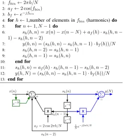
Algorithm 1 Goertzel andSGT algorithm implementation.

1: fbin←2πh/N 2: af ←2 cos(fbin) 3: bf ←e−jfbin

4: forh←1,number of elements infbin (harmonics) do 5: forn←1, N−1 do

6: sh(h, n) =x(n)−x(n−N) +af(h)·sh(h, n− 1)−sh(h, n−2)

7: y(h, n) = (sh(h, n)−sh(h, n−1)·bf(h))/N 8: sh(h, n−2) =sh(h, n−1)

9: sh(h, n−1) =sh(h, n)

10: end for

11: sh(h, n) =af(h)·sh(h, n−1)−sh(h, n−2) 12: y(h, N) = (sh(h, n)−sh(h, n−1)·bf(h))/N 13: end for

x x

Fig. 1. IIR implementation of the Goertzel algorithm for a single harmonic h. Black traces are the operations computed at each sample. For the standard Goertzel, blue traces represent the operations to be done at the last step (n= N), corresponding to lines11and12in Algorithm 1. Green lines represent the additional operations for theSGTimplementation. It has to be remarked, that for the case of theSGT, the output equation needs to be calculated at each sample (line7in Algorithm 1) _.

one fundamental cycle, assuming a 50Hz nominal frequency, is considered at10kHz sample rate, leading to a time window of 20ms and 200samples. With the proposed parameters, the calculations using the Goertzel approach are faster than the FFT alternative when the calculated number of harmonics is

M ≤ 8. The algorithm description in pseudo-code and the block diagram for the implementation are shown in Algorithm 1 and Fig. 1 respectively. At the implementation, thehinput variable contains the harmonic order of the sequences being analyzed.

In order to fully understand the SGT, it is useful to compare its dynamic response with respect to the standard Goertzel algorithm. The transfer function of the Goertzel algorithm in the z domain is given by (1), where ωh = 2πh/N, being h the harmonic order. The corresponding frequency response is shown in Fig. 2. As it can be seen from the frequency response, the Goertzel algorithm works as a resonator at the specified

ωh frequencies.

H_{g h}= 1−e

−jωh_z−1

1−2 cos(ωh)z−1_+z−2 (1)

[dB] -100

-50 0

freq [Hz]

-350 -150 50 250

[deg]

-180 -90 0 90 180

Fig. 2. Goertzel algorithm frequency response for a complex signal with harmonicsh= [1,−3,5,−7]. In blue the overall response is shown, in gray the response when the algorithm is tuned only forh= 1.

to H_{g h} and the second one to z−NH_{g h}. The corresponding frequency response is shown in Fig. 3.

H_{sg h}= 1−e

−jωh_z−1 _1−z−N

1−2 cos(ωh)z−1_+z−2 =Hg h 1−z

−N

(2)

[dB]

-100 -50 0

freq [Hz]

-350 -150 50 250

[deg]

-180 -90 0 90 180

Fig. 3. Sliding Goertzel algorithm frequency response for a complex signal with harmonicsh= [1,−3,5,−7]. In blue the overall response is shown, in gray the response when the algorithm is tuned only forh= 1.

III. SEQUENCE EXTRACTOR IMPLEMENTATION

Use of Goertzel-based techniques for sequence extraction requires to measure the grid phase voltages (van, vbn, vcn), and to transform them to the stationary reference frame (vαβ). From there, the real and the imaginary part vαβ =vα+jvβ are used as inputs to the Goerzel algorithm. A comparison for the impulse response and the poles and zeros map for both the standard Goertzel implementation and sliding approach is shown in Fig. 4. As it has been discussed, the differences are related to the duration of the impulse response. For the case of the standard Goertzel approach, the impulse response is a pure resonator at the frequency of the tracked harmonics. For the case of the sliding Goertzel, the impulse response duration is limited to the duration of the processing window (N samples), in the shown case corresponding to20ms.

For the validation of the system, the harmonics detailed in Table I are used. A comparison between the estimation given by the standard Goertzel and the SGT with respect to the

-1 0 1

-1 0 1

-1 0 1

time [s]

0 0.02 0.04 0.06 0.08

-1 0 1

-1 0 1

-1 0 1

Fig. 4. Impulse response and pole/zero map for the Goertzel method (top) and the Sliding Goertzel modification (bottom).N= 20,h= 1for a simpler representation.

TABLE I CONSIDERED HARMONICS.

Harmonic Order Mag (p.u.)

1 1

-5 0.2

7 0.2

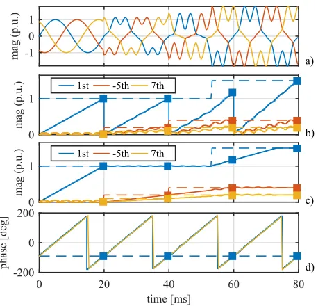
actual harmonic magnitudes and phases is shown in Fig. 5. As it can be seen, when the input signal is at steady state

a)

b)

c)

d)

mag (p.u.) -1 0 1

mag (p.u.)

0 1

1st -5th 7th

time [ms] -200

0 200

0 20 40 60 80

phase [deg]

mag (p.u.)

0 1

1st -5th 7th

Fig. 5. Sliding Goertzel estimation for a three phase system with the harmonic contents shown in Table I. The dotted lines correspond to the real value of each of the harmonics. The square dots represent the estimated value at the end of each block. a) waveforms, b) Goertzel and c) SGT estimation, d) phase.

discontinuous, being the current harmonic value only reached at the end of the current processing window and restarted at the beginning of the next one. Obviously, this invalidates the method to be directly used in converter real-time control ap-plications, as the one proposed in this paper. Alternatively, the

SGT approach represented in Fig. 5c) allows for a continuous estimation. This is the selected choice for our investigations. 2) The estimated magnitude needs the total number of samples and time,N = 200,t= 20ms, to converge to the correct value. This would raise an unacceptable delay when the estimation is used as a feedback signal. However, it can be also seen that the evolution of the fundamental component (1st harmonic) estimation is linear during the estimation window and barely affected by the harmonic content.

In order to overcome 2), this paper proposes to incorpo-rate a predictive SGT implementation, namely P −SGT, that improves the convergence speed and, at the same time, avoids the extra calculations derived from the overlapping. The predictive behavior is implemented by a two-step algorithm. Firstly, a linear sliding least squares estimation (LSE) is run over the output of each SGT sample. This will lead to a linear representation of the corresponding datapoints. It must be remarked that being the output values of the

SGT complex, two different least squares estimation can be obtained: one for the module and another one for the phase. Even considering this linear condition both for the magnitude and the phase estimation, at this paper the phase estimation is directly obtained from the SGT algorithm due to the fact that an accurate phase estimation can be obtained before each window is completed. Secondly, the module value at the end of the estimation window is predicted. This last step is implemented at each step by again considering the linear evolution expressed in (3)

b

y[N] =y[n] +mle[n]·[N−n] (3)

, where mle[n] is the moving average slope estimated by the

LSE approach,N the window size andn the actual sample. A graphical description for the algorithm is shown in Fig. 6.

N 2N [n]

prediction horizon n=N-n

[n]

least squares estimation

prediction

Fig. 6. Graphical representation of the proposed predictive algorithm. The slope at each of the points is filtered by a moving average filter for reducing the derivative noise.

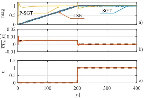
The simulation results for the proposed methods are shown in Fig. 7. As it can be seen, the results obtained by the

P −SGT approximation notably improve the convergence estimation speed. However, even with the averaged slope cal-culation, a transient can be observed at the beginning of each processing window. This behavior is inherent to the involved derivative process. By comparing the smooth transitions given by theSGT, it can be deduced that both estimations can work

mag

0 0.5 1

-0.01 0 0.01 0.02

[n]

0 100 200 300 400

n

0 0.5 1 1.5

a)

b)

c)

P-SGT _LSE SGT

Fig. 7. ProposedP−SGT implementation. a) evolution of the magnitude. SGT in blue,LSE in red andP −SGT in yellow.. b) evolution of the predicted slope, c) evolution of the predicted offset. A window ofN= 200 has been used for demonstration purposes.

in a complementary approach. The combined estimation will be based on the rate of change in the SGT estimation. As previously discussed, during the SGT convergence time, the estimation will exhibit a mostly linear change. On the contrary, once the estimation has reached the final value, it will have a mostly zero variation. Based on that, the P −SGT will be favored during the transients, whereas the classical SGT

will be mostly used at the steady state. This idea will be mathematically developed and numerically evaluated during the next section.

A. CombinedSGT andP−SGT estimation

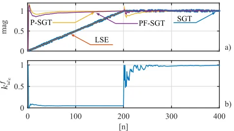
Considering the performance of both theSGT and theP− SGT strategies shown in Fig. 7, it is proposed to combine both methods, leading to the so calledP F−SGT, for getting an enhanced estimation. For the fusion rule, (4) is proposed.

X_hωpf−sgt

e =X

p−sgt

hωe ·(1−k

f

hωe) +X

sgt hωe·(k

f

hωe) (4)

The value of the fusion gain,kf_hω

e, in (4) is given by (5).

kf_hω

e =exp

−abs mavg(4X

sgt hωe) max(4Xsgt

hωe)

!! ·ghωe

(5)

Variables in (4), (5) are defined as follows:

• X_hωsgt

e. SGT estimation of harmonic component h at

fundamental frequency ωe for variableX. • X_hωp−sgt

e .P−SGT estimation of harmonic componenth

at fundamental frequency ωe for variableX. • X_hωpf−sgt

e . P F −SGT estimation of the harmonic

com-ponenthat fundamental frequencyωefor variable X. • 4X_hωsgt

e is the rate of change of the module of the

estimated harmonic components by the SGT algorithm. It is calculated as the difference between the module of the actual sample minus the previous one.

• mavg. Moving average function. A window of N sam-ples is used for the calculation.

• ghωe. Gain of the exponential function used for tuning

the fusion system.

Evolution of the estimation and the adaptive gain is shown in Fig. 8. As clearly shown, the fusion helps on removing the transient at the beginning of each of the processing windows. Time constant for the fusion estimation depending on the value of the fusion gainghωeis shown in 9, where a parameter sweep

of ghωe (between 1 and 6) is performed. As it can be seen,

for the selected magnitude steps, values larger thanghωe >4

do not contribute to an improved transient response.

mag

0 0.5 1

[n]

0 100 200 300 400

0 0.5 1

a)

b) P-SGT

LSE

SGT PF-SGT

Fig. 8. Proposed fusion mechanism. a) evolution of the module. b) evolution of the gain.ghωe= 5,max(4X

sgt

hωe) = 5.5e−3

time [s]

0.75 0.8 0.85 0.9 0.95 1 1.05

mag [p.u.]

0.7 0.8 0.9 1

g

hω

e

1 1.5 2 2.5 3 3.5 4 4.5 5 6

τ

[ms]

0 5 10

step t=0.8 step t=0.9

𝑔_{hω𝑒 =1}

𝑔_hω𝑒= 6

Fig. 9. Variation of the fusion time constant with respect to the fusion gain. On top, the response of the proposed fusion mechanism to two different step changes is shown, on bottom the calculated time constant.

B. Frequency estimation

When the proposed P F−SGT method is applied for the estimation of grid voltages and currents, frequency changes must be considered. As known, frequency domain methods based on the DFT assume the periodicity of the signal and are affected by the discrete resolution. However, when used for the analysis of signals coming from a real-time application, this assumption is not longer valid. The effect of the signal being not periodic, together with the discrete resolution, will

cause spectral leakage, affecting both the phase and magnitude of the estimated components. Often, windowing techniques (both in time and frequency domain) are applied in order to reduce the impact. Unfortunately, this procedure also affects the magnitude and the phase of the extracted components and often additional compensation is needed. A different approach, is to optimize the number of samples needed for the calculation (200 by default in our implementation) depending on the fundamental frequency, so an integer number of cycles is acquired at each processing window. For this paper, and con-sidering that only the harmonics of the fundamental frequency needs to be isolated, an even simpler approach has been used. By selecting a coarse spectral resolution of 50Hz, spectral leakage is avoided when deviations from the fundamental frequency appears. The drawbacks of this procedure are that, as commented in Section V-B, a bounded steady state error for the phase will appear and that any other disturbance signal falling within the band of [25−75]Hz will be affecting the estimation. Additionally, also in Section V-B, an adaptive fre-quency method is considered for those applications requiring a zero-steady-state phase error.

C. Magnitude estimation errors due to theLSE algorithm

The magnitude estimation using the proposedLSE method over a N-length window depends on the sample where the disturbance occurs (0 < n < N −1). This is due to the slope averaging define in (3). The average leads to magnitude estimation errors if any change in the signal magnitude oc-curs during the LSE calculation period. Fig. 10 shows the magnitude estimation for two different cases. In the first one (blue trace), the disturbances occur at t = [0,60]ms, which correspond in both cases to n = 0 sample at processing windows1and4. Under that conditions, the predicted slope,m

and offset,n, are correctly estimated. In the second case (red trace), the magnitude steps are commanded at t= [0,50]ms, corresponding to n = [0, N/2] samples respectively. As shown, for the t = 50ms step, the slope prediction starts to react at the step time but, because of the average calculation, the value by the end of the processing window, t = 60ms, is half of the expected value. After that, during the next processing window starting att= 60ms, the slope is correctly adapted untilt= 70ms, time at which the average calculation makes the prediction to decrease, reaching half of the expected value at t = 80ms. Similar explanations can be given to the offset calculation. The two explained cases, cover the minimum and maximum estimation errors. The maximum error will happen when an step change happens at half the processing window and will be equal to half the correct value.

p-sgt mag [p.u.] 0 1 2

m [x10

-3 ]

0 2 4 6

time [ms]

0 20 40 60 80

n

0 1 2

Fig. 10. Prediction errors due to the averaging window problem. a) SG estimated magnitude for two different cases. Blue: magnitude changes aligned with samplen= 0at each window. Red: magnitude change att= 50ms at samplen=N/2. b) and c) estimated slopes and offsets for the two cases.

the value of the fundamental component from 1p.u to1.5p.u is commanded at t = 50ms, corresponding to n=N/2. As shown in Fig. 11b), the output of a slope change detector instantaneously reacts to the change. This fact will be used as a trigger mechanism for resetting the estimation window. The trigger signal is based on the absolute value of the derivative of the slope given by the SGT, and it is shown in Fig. 11b) depicted in blue. By comparing with a trigger level, represented by the red slashed line, the processing window can be reset. The results for the predicted slope and offset are depicted in red in Figs. 11c) and 11d) respectively. Finally, the estimated output is shown in Fig. 11e). Clearly the estimation tracks the correct values in around5ms, which is an excellent response time. As a comparison, the tracked slope and offset using the standard approach is shown in blue.

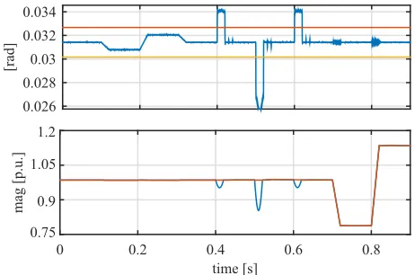
D. Phase-jump detection and magnitude correction

An adverse effect that noticeably affects to the magnitude and frequency estimation is the occurrence of a phase jump. This subsection shows a simple technique that detects a phase jump and corrects its effects in the estimated magnitude. The main underpinning idea is to check if the phase difference between the actual phase angle estimation and the previous one falls within the grid code limits. An acceptable frequency deviation from the nominal value has been selected to be

ωerr = 2·2πrad/s. According to that, the phase difference between the actual phase estimation and the previous one should fall within the phase limits defined by (6), whereTsis the sample time and Psthe phase difference.

(ωe−ωerr)·Ts< Ps<(ωe+ωerr)·Ts (6)

Thus, if a phase jump is detected, the magnitude estimation at the previous sample is used. Alternatively, a low-pass version of the voltage complex vector could be used, but this solution requires more computational effort at no extra advantage. Fig. 12 shows the proposed correction mechanism

mag [p.u.]-1 0 1

M th

[x10

-3 ]

0 5

m [x10

-3 ]

0 2 4 6

n

0 1 2

time [ms]

0 20 40 60 80

mag [p.u.] 0 1

a)

b)

c)

d)

e)

Fig. 11. Correction of window averaging errors. a) voltage to neutral waveforms, b) slope change detector, c) LSE slope, d) LSE offset, e) estimated output. In c) and d) blue and red represents the slope and offset obtained by theLSEwithout and with the proposed modification respectively.

[rad]

0.026 0.028 0.03 0.032 0.034

time [s]

0 0.2 0.4 0.6 0.8

mag [p.u.]

1.2

0.9 1.05

0.75

Fig. 12. Compensation of magnitude estimation during three phase-jumps. On top, the phase-jumps are represented in blue and the limits given by (6) in red and yellow. Phase-jumps occur at t = [0.4,0.5,0.6] s. On bottom, the estimated magnitude before (blue) and after (red) the correction is implemented.

compared to the magnitude variation before the compensation.

E. Digital signal processing

The digital signal processing needed for the implementation of the proposedP F−SGT method as well as its use for the current control of a grid-tied converter is explained in Fig. 13. On the left-side, the input to the algorithm is thevαβ voltage complex vector measured at the point of common coupling. The output of the method are the complex components of the estimated harmonics v_{αβ h}

1···hn as well as the phase of the

main harmonic, _∠v_{αβ h}

1. In the case an adaptive frequency

Fusion

current control PF

SGT

LSE SGT

Fig. 13. Digital signal processing. Left-side, estimation of voltage harmonics. Right-side. Use of the estimated voltages in the internal current-loop control.

the use of the estimated components for the current control implementation is shown. The estimated phase is used as the rotation angle for theαβ−→dqtransformation. The estimated grid voltage harmonic components can be used as a feed-forward added at the output of the current control.

The computation burden of the proposed method can be calculated by computing the needed floating point operations and the memory needs. The number of floating point opera-tions considering four harmonics is around2200. Considering the number of cycles for each floating point operation based on a T M S320F28335 controller with a 150MHz clock, it leads to a computational time lower than 60µs. Regarding the memory needs, a buffer of N+ 1 samples is needed for the calculation of the SGT plus some additional room for the scalar variables. Considering together the processing and memory needs, it is concluded that the proposed method has a moderate computational burden for modern digital signal controllers.

IV. OFF-LINESYSTEM EVALUATION

The initial evaluation of the proposed sequence estimator has been done using a programmable voltage source (2210 TC-ACS-50-480-400 from Regatron) to create the different grid conditions. Different steps at the magnitude, phase and frequency of the signal are considered as well as the behavior with and without additional harmonic content. The data is acquired at 1Ms/s sample rate by an scope and later down-sampled to 10kHz. The down-sampled signal is processed in Matlab/Simulink using the same code implementation later to be used during the on-line test.

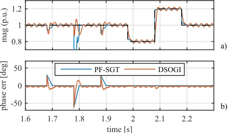
The results for the tracked grid voltage’s magnitude and phase using the P F −SGT are shown in Fig 14 and 15. The different events at the source signal are repeated twice. During the first interval (t = 0−1.2 s), no harmonics were included. At the second one, the harmonics indicated at Table I are considered. Moreover, starting att= 1.5s, a dc offset is added at the output of the voltage sensors. Dc-offset values are

Vu= 10V,Vv = 5V,Vw=−5V. The events are scheduled as follows: 1)Magnitude. Att= 0.8 s andt= 0.9s it changes to0.8and1.2p.u. The same change is observed att= 1.98s andt= 2.08s. 2)Frequency. Att= 0.2s andt= 0.3s, the rated50Hz frequency is changed to49and51Hz respectively. Same pattern is reproduced at t = 1.38 s and t = 1.48 s. 3) Phase. At t = 0.5, t = 0.6, t = 0.7 s phase jumps of 30,−60,30deg. are induced. Same pattern is observed att= 1.68,1.78,1.88 s. At the graph, the behavior of the proposed method is tested compared to the DSOGI implementation. The

tuning of the DSOGI has been done according to the optimal parameters indicated by its authors [9]. As it can be seen, the proposed method shows a better immunity to harmonics and faster response to the considered changes with the exception of the phase change att= 0.6 and1.78 s. This is due to the correction explained in (6) not being considered for the initial evaluation. It is specially remarkable the improvement of the proposed method when DC components are considered.

a)

b) mag (p.u.) -1

0 1

time [s] mag (p.u.) 0.8

1 1.2

PFSGT DSOGI 1st

2 1.5

1 0.5

0

1.15 time [s] 1.2 -1

0 1

Fig. 14. Off-line system evaluation. Comparison of theP F−SGT method with respect to the ideal1st _{harmonic and the DSOGI implementation. a)}

time domain waveforms, b) module estimation.

a)

b) mag (p.u.) 0.8

1 1.2

time [s]

1.6 1.7 1.8 1.9 2 2.1 2.2

phase err [deg] -50 0

50 PF-SGT DSOGI

Fig. 15. Off-line system evaluation. Detail on the comparison of the P F−SGT method with respect to the ideal1st_{harmonic and the DSOGI}

implementation. a) module, b) phase error_.

A. Performance under unbalanced conditions

Fig. 16 shows the performance of the proposed technique and the DSOGI method under unbalanced conditions. Att= 0.2 s, phase b of the input three-phase voltage falls to 0.7 p.u. (Fig. 16). The same disturbances as the previous tests are aplied under unbalanced conditions: frequency deviation test is performed between t = 0.4 s and t = 0.6 s, phase jump test is performed between t= 0.7 s andt= 0.9 s and finally magnitude deviations test is performed betweent= 1.0s and

t = 1.2 s. As it can be observed, the obtained results match with that retrieved in the previous tests. In this regard, the proposed method shows a better tracking capabilities under all tested disturbances.

B. Closed-loop behavior

mag [p.u.] -1 0 1

mag [p.u.] 0.8 1

time [s]

0.2 0.4 0.6 0.8 1 1.2

phase err [deg] -10 0 10

PF-SGT DSOGI

mag [p.u.] -1 0 1

mag [p.u.] 0.8 1

time [s]

0.2 0.4 0.6 0.8 1 1.2

phase err [deg] -10 0 10

PF-SGT DSOGI

mag [p.u.] -1 0 1

mag [p.u.] 0.8 1

time [s]

0.2 0.4 0.6 0.8 1 1.2

phase err [deg] -10 0 10

PF-SGT DSOGI

Fig. 16. Off-line system evaluation. Comparison between the DSOGI and the proposedP F −SGT method under unbalanced conditions. From top to bottom: a) grid voltages, b) grid voltage magnitude, c) grid voltage phase error.

TABLE II

APPROXIMATION PARAMETERS.

Method fn(Hz) ξ

DSOGI 60.5 √

(2)·3 2 PF-SGT 8600 p(2)·8

PI controller is used while the plant has been modeled as a RL circuit. Since both the DSOGI and the PF-SGT methods involve nonlinear systems, their transfer functions have been approximated by 2nd _{order systems as shown in Fig. 17. The} results of the approximation procedure are shown in Table II, whereωn andξare the natural frequency and damping factor of each method respectively.

0.96 0.98 1 1.02 1.04

mag [p.u.] 1 1.25 1.5

DSOGI aprox

time [s]

0.995 0.9975 1 1.0025 1.005

mag [p.u.] 1 1.25 1.5

PF-SGT aprox

Fig. 17. Aproximation of a) DSOGI and b) PF-SGT methods

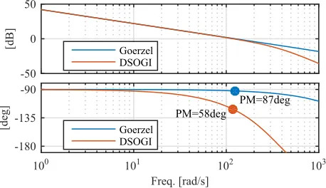
For both techniques, the current control loop is tunned by using a zero-pole cancellation technique, its bandwidth being set to (20 Hz). The phase margin of the system is used as a figure of merit to analyze the stability of the current control loop. In this regard, a limit of 60 deg will be considered to assure stability.

Fig. 18 shows theG(s)H(s)Bode plots for a bandwidth in the current control loop of20Hz. It can be observed that the

[dB]

-50 0 50

Goerzel DSOGI

Freq. [rad/s]

100 101 102 103

[d

eg]

-180 -135 -90

Goerzel DSOGI

PM=87deg PM=58deg

Fig. 18. G(s)H(s)Bode Plot for DSOGI and proposed methods. Current Control BandwidthBWI= 20Hz

phase margin of the system including the DSOGI method is 58deg, while it is≈87degwhen the PF-SGT method is used under the same bandwidth (see Fig. 18). This clearly shows the bandwidth limit of the current control loop when a DSOGI method is used.

The closed-loop current control relevant signals are shown in Fig. 19. Reference tracking capabilities in the synchronous reference frame has been tested. The grid voltage was ac-quired as previously explained and the down-sampled voltage data was used in a real-time Simulink simulation. The same sequence than for the open-loop results shown in Fig. 14 has been used. The relevant parameters for the setup are: filter values: L = 5mH, R = 0.2Ω, switching frequency fsw = 10kHz, current control bandwidth 20Hz. As clearly shown, the proposed method shows a better transient response and harmonic rejection capabilities than the DSOGI alternative. Moreover, the bandwidth was set to such a low value in order to keep stable the DSOGI-based current control.

[V]

-500 0 500

[A]

-50 0 50

time [s]

0 0.5 1 1.5 2

kf

0 0.5 1

a)

b)

c)

Fig. 19. Off-line system evaluation

. Close loop comparison between the DSOGI and the proposedP F−SGT methods. a) grid voltages, b) grid currents, c) adaptive fusion gain for the P F−SGT method.

V. ON-LINESYSTEM EVALUATION

in Fig. 20. The setup is composed by two Triphase power modules PM15F42C and PM90F60C and a set of passive loads. The PM90F60C module is used as a grid voltage emulator for creating the different grid scenarios, modifying the magnitude, phase, frequency and harmonic content of the voltage signal. The PM15F42C module is integrated in the system operating as a constant power controlled battery energy storage system. The proposed algorithms are processed online in the PM15F42C control unit using the voltage measurements at the point of common coupling (PCC). The experimental results use the DSOGI algorithm as the base case for the comparison.

Fig. 20. Setup used for the experimental validation. Two converters are coupled together, PM90F60C unit is used to create the varying grid conditions and PM15F42C runs the proposed estimation method.

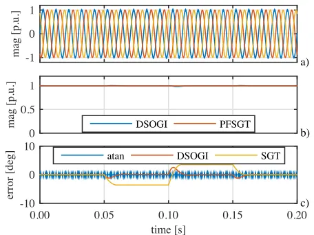
A. Variation of grid voltage magnitude

Variations of the grid voltage magnitude from 1 to 0.8 p.u. at t = 0.1 s and from 0.8 to 1.15 p.u. at t = 0.2 are considered. Results both without and with the h5 = 5%, h7= 5%additional harmonics are shown in Fig. 21 and Fig. 22 respectively. As shown, the proposed method has a faster dynamic response as well as a higher harmonic robustness, both for the magnitude and the phase estimation.

B. Variation of grid voltage frequency

Variations of grid voltage frequency from 50 to 49 Hz at t = 0.1 s and from 49 to 51 Hz at t = 0.2 are considered. Results both without and with the h5 = 5%, h7 = 5% additional harmonics are shown in Fig. 24 and Fig. 25 respectively. As shown, the proposed method has a better magnitude response but a worse phase as there is an steady state error in the phase estimation. The reason is the considered frequency resolution. As explained before, a coarse frequency resolution of 50Hz. has been selected for this work. This implies that any deviation smaller than 50Hz can not be measured and the difference between the real grid frequency and the fundamental harmonic is directly coupled to a phase and a magnitude error. The maximum errors have been numerically evaluated as shown in Fig. 23. As it can be seen, both the error in magnitude and phase are small for variations between [46,54]Hz. The maximum phase error can

mag [p.u.] -1 0

a)

mag [p.u.]

0 0.5 1

DSOGI PFSGT

b)

time [s]

0.00 0.05 0.10 0.15 0.20

error [deg]

-10 0 10

atan DSOGI SGT

c) mag [p.u.] -1

0 1

a)

mag [p.u.]

0 0.5 1

DSOGI PFSGT

b)

time [s]

0.00 0.05 0.10 0.15 0.20

error [deg]

-10 0 10

atan DSOGI SGT

c) mag [p.u.] -1

0 1

a)

mag [p.u.]

0 0.5 1

DSOGI PFSGT

b)

time [s]

0.00 0.05 0.10 0.15 0.20

error [deg]

-10 0 10

atan DSOGI SGT

c)

Fig. 21. On-line system evaluation. Comparison between the DSOGI and the proposedP F−SGTmethod for a magnitude step change. No harmonics are injected. From top to bottom: a) grid voltages, b) grid voltage magnitude, c) grid voltage phase error. Note thatatanrefers to the inverse-tangent function.

mag [p.u.] -1

0 1

a)

mag [p.u.]

0 0.5 1

DSOGI PFSGT

b)

time [s]

0.00 0.05 0.10 0.15 0.20 0.25 0.30

error [deg]

-10 0 10

atan DSOGI SGT

c)

Fig. 22. On-line system evaluation. Comparison between the DSOGI and the proposedP F−SGT method for a magnitude step change. Harmonics as listed in Table I are injected. From top to bottom: a) grid voltages, b) grid voltage magnitude, c) grid voltage phase error.

be approximated by the linear expression shown in (7), where max (ωerr)is the maximum frequency error in rad/s and fe the grid frequency in Hz.

maxθerr=

max (ωerr)·180 fe·2π

(7)

mag err [p.u.] -0.05

0 0.05

freq [Hz]

46 48 50 52 54

phase err [deg] -20

0 20

num eval eq (7)

Fig. 23. Effect of grid frequency variation over the estimated magntitude (top) and phase (bottom). Phase error is compared against the linear approximation in (7).

mag [p.u.] -1 0 1

a)

mag [p.u.]

0 0.5 1

DSOGI PFSGT

b)

time [s]

0.00 0.05 0.10 0.15 0.20

error [deg]

-10 0 10

atan DSOGI SGT

c) mag [p.u.] -1

0 1

a)

mag [p.u.]

0 0.5 1

DSOGI PFSGT

b)

time [s]

0.00 0.05 0.10 0.15 0.20

error [deg]

-10 0 10

atan DSOGI SGT

c) mag [p.u.] -1

0 1

a)

mag [p.u.]

0 0.5 1

DSOGI PFSGT

b)

time [s]

0.00 0.05 0.10 0.15 0.20

error [deg]

-10 0 10

atan DSOGI SGT

c)

Fig. 24. On-line system evaluation

. Comparison between the DSOGI and the proposed

P F −SGT method for a frequency step change. No harmonics are injected. From top to bottom: a) grid voltages,

b) grid voltage magnitude, c) grid voltage phase error.

the coefficients for the Goertzel algorithm have to be updated in real time. The experimental results when the adaptation mechanism is used are shown in Fig. 27. Comparing the phase error with respect to Fig. 25, the phase jump is corrected, achieving a zero phase error in steady state.

N =round _2π

ωe·Ts

(8)

C. Variation of grid voltage phase

Variations of grid voltage phase from 0 to 30 deg. at

t= 0.05 s, from30 to−30 deg att= 0.1 and from−30to 0 deg att= 0.15s are considered. Results both without and with the h5= 5%,h7 = 5%additional harmonics are shown in Fig. 28 and Fig. 29 respectively. The proposed method has similar results compared to DSOGI when no additional harmonics are considered and an improved response under harmonic conditions.

mag [p.u.] -1

0 1

a)

mag [p.u.]

0 0.5 1

DSOGI PFSGT

b)

time [s]

0.00 0.05 0.10 0.15 0.20

error [deg]

-10 0 10

atan DSOGI SGT

c) mag [p.u.] -1

0 1

a)

mag [p.u.]

0 0.5 1

DSOGI PFSGT

b)

time [s]

0.00 0.05 0.10 0.15 0.20

error [deg]

-10 0 10

atan DSOGI SGT

c) mag [p.u.] -1

0

a)

mag [p.u.]

0 0.5 1

DSOGI PFSGT

b)

time [s]

0.00 0.05 0.10 0.15 0.20

error [deg]

-10 0 10

atan DSOGI SGT

c)

Fig. 25. On-line system evaluation. Comparison between the DSOGI and the proposedP F−SGT method for a frequency step change. Harmonics as listed in Table I are injected. From top to bottom: a) grid voltages, b) grid voltage magnitude, c) grid voltage phase error.

mag [pu]

0.5 1

time [s]

0 0.2 0.4 0.6 0.8 1 1.2 1.4

error [deg] -20

0 20

1.25 1.26 1.27

Fig. 26. On-line system evaluation. Effect of grid frequency variation over the magnitude (top) and phase (bottom). Goertzel algorithm is tuned for50Hz and three different cases are represented:50Hz (blue),49Hz (yellow),51Hz (red). Theoretical limits for the phase according to expression (7) are marked dotted.

VI. CONCLUSION

This paper has introduced a new predictive estimation technique for grid-tied converters based on a frequency-based method. To the author’s best knowledge, the proposed method using a modification of the Sliding Goertzel Transformation has not been used before for grid phase tracking in power con-verters. The proposedP F−SGT method has been evaluated with respect to a consolidated alternative, the DSOGI, showing a superior performance in terms of dynamic response and disturbance rejection. It is particular remarkable the immunity to DC offsets as well as to changes at the grid frequency. The proposed algorithm has been validated by both simulation and experimental results. The impact of the phase estimation and harmonic decoupling in a closed-loop current control implementation has also been evaluated, being the proposed

mag [p.u.] -1 0 1 a) mag [p.u.] 0 0.5 1 DSOGI PFSGT b) time [s]

0.00 0.10 0.20 0.30 0.40

error [deg]

-10 0 10

atan DSOGI SGT

c) a)

b)

c)

mag [p.u.] -1

0 1 a) mag [p.u.] 0 0.5 1 DSOGI PFSGT b) time [s]

0.00 0.10 0.20 0.30 0.40

error [deg]

-10 0 10

atan DSOGI SGT

c) a)

b)

c)

mag [p.u.] -1

0 a) mag [p.u.] 0 0.5 1 DSOGI PFSGT b) time [s]

0.00 0.10 0.20 0.30 0.40

error [deg]

-10 0 10

atan DSOGI SGT

c) a) b) c) a) b) c)

Fig. 27. On-line system evaluation. Comparison between the DSOGI and the proposedP F−SGTmethod for a frequency step change when an adaptive frequency is used. Harmonics as listed in Table I are injected. From top to bottom: a) grid voltages, b) grid voltage magnitude, c) grid voltage phase error.

mag [p.u.] -1 0 1 a) mag [p.u.] 0 0.5 1 DSOGI PFSGT b) time [s]

0.00 0.05 0.10 0.15 0.20

error [deg]

-10 0 10

atan DSOGI SGT

c)

mag [p.u.] -1 0 1 a) mag [p.u.] 0 0.5 1 DSOGI PFSGT b) time [s]

0.00 0.05 0.10 0.15 0.20

error [deg]

-10 0 10

atan DSOGI SGT

c)

mag [p.u.] -1 0 1 a) mag [p.u.] 0 0.5 1 DSOGI PFSGT b) time [s]

0.00 0.05 0.10 0.15 0.20

error [deg]

-10 0 10

atan DSOGI SGT

c)

Fig. 28. On-line system evaluation. Comparison between the DSOGI and the proposedP F −SGT method for a phase step change. No harmonics are injected. From top to bottom: a) grid voltages, b) grid voltage magnitude, c) grid voltage phase error.

REFERENCES

[1] C. Blanco, D. Reigosa, J. C. Vasquez, J. M. Guerrero, and F. Briz, “Virtual admittance loop for voltage harmonic compensation in micro-grids,”IEEE Transactions on Industry Applications, vol. 52, no. 4, pp. 3348–3356, July 2016.

[2] J. W. Simpson-Porco, Q. Shafiee, F. Dörfler, J. C. Vasquez, J. M. Guerrero, and F. Bullo, “Secondary frequency and voltage control of islanded microgrids via distributed averaging,” IEEE Transactions on Industrial Electronics, vol. 62, no. 11, pp. 7025–7038, Nov 2015. [3] E. Twining and D. G. Holmes, “Grid current regulation of a three-phase

voltage source inverter with an lcl input filter,”IEEE Transactions on Power Electronics, vol. 18, no. 3, pp. 888–895, May 2003.

[4] S. Yang, Q. Lei, F. Z. Peng, and Z. Qian, “A robust control scheme for grid-connected voltage-source inverters,” IEEE Transactions on Industrial Electronics, vol. 58, no. 1, pp. 202–212, Jan 2011. [5] J. C. Vasquez, J. M. Guerrero, M. Savaghebi, J. Eloy-Garcia, and

R. Teodorescu, “Modeling, analysis, and design of stationary-reference-frame droop-controlled parallel three-phase voltage source inverters,” IEEE Transactions on Industrial Electronics, vol. 60, no. 4, pp. 1271– 1280, April 2013.

[6] S. Golestan, J. M. Guerrero, and J. C. Vasquez, “Three-phase plls: A review of recent advances,”IEEE Transactions on Power Electronics, vol. 32, no. 3, pp. 1894–1907, March 2017.

mag [p.u.] -1 0 1 a) mag [p.u.] 0 0.5 1 DSOGI PFSGT b) time [s]

0.00 0.05 0.10 0.15 0.20

error [deg]

-10 0 10

atan DSOGI SGT

c) mag [p.u.] -1

0 1 a) mag [p.u.] 0 0.5 1 DSOGI PFSGT b) time [s]

0.00 0.05 0.10 0.15 0.20

error [deg]

-10 0 10

atan DSOGI SGT

c) mag [p.u.] -1

0 a) mag [p.u.] 0 0.5 1 DSOGI PFSGT b) time [s]

0.00 0.05 0.10 0.15 0.20

error [deg]

-10 0 10

atan DSOGI SGT

c)

Fig. 29. On-line system evaluation. Comparison between the DSOGI and the proposedP F−SGT method for a phase step change. Harmonics as listed in Table I are injected. From top to bottom: a) grid voltages, b) grid voltage magnitude, c) grid voltage phase error.

[7] F. D. Freijedo, J. Doval-Gandoy, O. Lopez, and E. Acha, “A generic open-loop algorithm for three-phase grid voltage/current synchronization with particular reference to phase, frequency, and amplitude estimation,” IEEE Transactions on Power Electronics, vol. 24, no. 1, pp. 94–107, Jan 2009.

[8] S. Golestan, A. Vidal, A. G. Yepes, J. M. Guerrero, J. C. Vasquez, and J. Doval-Gandoy, “A true open-loop synchronization technique,”IEEE Transactions on Industrial Informatics, vol. 12, no. 3, pp. 1093–1103, June 2016.

[9] P. Rodriguez, A. Luna, M. Ciobotaru, R. Teodorescu, and F. Blaabjerg, “Advanced grid synchronization system for power converters under unbalanced and distorted operating conditions,” inIECON 2006 - 32nd Annual Conference on IEEE Industrial Electronics, Nov 2006, pp. 5173– 5178.

[10] P. Rodriguez, R. Teodorescu, I. Candela, A. Timbus, M. Liserre, and F. Blaabjerg, “New positive-sequence voltage detector for grid synchro-nization of power converters under faulty grid conditions,” in2006 37th IEEE Power Electronics Specialists Conference, June 2006, pp. 1–7. [11] A. M. Gole and V. K. Sood, “A static compensator model for use with

electromagnetic transients simulation programs,”IEEE Transactions on Power Delivery, vol. 5, no. 3, pp. 1398–1407, Jul 1990.

[12] C. Blanco, D. Reigosa, F. Briz, and J. M. Guerrero, “Synchronization in highly distorted three-phase grids using selective notch filters,” in 2013 IEEE Energy Conversion Congress and Exposition, Sept 2013, pp. 2641–2648.

[13] X. Guo, W. Wu, and Z. Chen, “Multiple-complex coefficient-filter-based phase-locked loop and synchronization technique for three-phase grid-interfaced converters in distributed utility networks,” Industrial Electronics, IEEE Transactions on, vol. 58, no. 4, pp. 1194–1204, April 2011.

[14] C. Blanco, D. Reigosa, F. Briz, J. M. Guerrero, and P. Garcia, “Grid synchronization of three-phase converters using cascaded complex vec-tor filter pll,” in2012 IEEE Energy Conversion Congress and Exposition (ECCE), Sept 2012, pp. 196–203.

[15] F. D. Freijedo, A. G. Yepes, O. Lopez, A. Vidal, and J. Doval-Gandoy, “Three-phase plls with fast postfault retracking and steady-state rejection of voltage unbalance and harmonics by means of lead compensation,” IEEE Transactions on Power Electronics, vol. 26, no. 1, pp. 85–97, Jan 2011.

[16] S. Golestan, J. M. Guerrero, A. Vidal, A. G. Yepes, and J. Doval-Gandoy, “Pll with maf-based prefiltering stage: Small-signal modeling and perfor-mance enhancement,”IEEE Transactions on Power Electronics, vol. 31, no. 6, pp. 4013–4019, June 2016.

[17] C. Blanco, D. Reigosa, F. Briz, and J. M. Guerrero, “Quadrature signal generator based on all-pass filter for single-phase synchronization,” in 2014 IEEE Energy Conversion Congress and Exposition (ECCE), Sept 2014, pp. 2655–2662.

[19] E. Jacobsen and R. Lyons, “The sliding dft,”IEEE Signal Processing Magazine, vol. 20, no. 2, pp. 74–80, Mar 2003.

[20] ——, “An update to the sliding dft,”IEEE Signal Processing Magazine, vol. 21, no. 1, pp. 110–111, Jan 2004.

[21] C. Blanco, P. García, A. Navarro-Rodríguez, and M. Sumner, “Predictive frequency-based sequence estimator for control of grid-tied converters under highly distorted conditions,” in 2017 IEEE Energy Conversion Congress and Exposition (ECCE), Oct 2017, pp. 2940–2947. [22] G. Goertzel, “An Algorithm for the Evaluation of Finite Trigonometric