Application of Advanced Stated Preference Design Methodology

(1)

White Rose Research Online URL for this paper:

http://eprints.whiterose.ac.uk/2109/

Monograph:

Clark, S.D. and Toner, J.P. (1997) Application of Advanced Stated Preference Design

Methodology. Working Paper. Institute of Transport Studies, University of Leeds , Leeds,

UK.

Working Paper 485

[email protected]

Reuse

Unless indicated otherwise, fulltext items are protected by copyright with all rights reserved. The copyright exception in section 29 of the Copyright, Designs and Patents Act 1988 allows the making of a single copy solely for the purpose of non-commercial research or private study within the limits of fair dealing. The publisher or other rights-holder may allow further reproduction and re-use of this version - refer to the White Rose Research Online record for this item. Where records identify the publisher as the copyright holder, users can verify any specific terms of use on the publisher’s website.

Takedown

If you consider content in White Rose Research Online to be in breach of UK law, please notify us by

(2)

White Rose Research Online

http://eprints.whiterose.ac.uk/

Institute of Transport Studies

University of Leeds

This is an ITS Working Paper produced and published by the University of

Leeds. ITS Working Papers are intended to provide information and encourage

discussion on a topic in advance of formal publication. They represent only the

views of the authors, and do not necessarily reflect the views or approval of the

sponsors.

White Rose Repository URL for this paper:

http://eprints.whiterose.ac.uk/

2109

Published paper

Stephen Clark and Jeremy Toner (1997)

Application of Advanced Stated

Preference Design Methodology.

Institute of Transport Studies, University of

Leeds, Working Paper 485

(3)

EPSRC Research Working Paper

APPLICATION OF ADVANCED STATED PREFERENCE DESIGN

METHODOLOGY

Stephen Clark and Jeremy Toner

Document Control Information

Title

: APPLICATION OF ADVANCED STATED PREFERENCE DESIGN

METHODOLOGY

Authors

:

Stephen Clark and Jeremy Toner

Reference Number

:

9612/01

Version

:

1.0 Date

: 14

February

1997

Distribution

:

SDC, JPT

Availability

:

Unrestricted

File

:

E:\HOME\SP\WP485.WP6

Authorised by

:

Stephen Clark

(4)

ITS Working Paper 485

ISSN 0142-8942

December 1996

APPLICATION OF ADVANCED STATED PREFERENCE

DESIGN METHODOLOGY

SD Clark

JP Toner

This work was undertaken on a project sponsored by the Engineering and Physical Sciences

esearch Council (Grant Ref: GR/J81242)

R

(5)

ABSTRACT... 1

1 BACKGROUND ... 1

2 MODELLING ... 3

3 NEW DESIGN METHODOLOGY ... 4

4 TWO

VARIABLES... 5

4.1 PRODUCING THE DESIGN ... 5

4.2 TESTING THE DESIGN... 9

4.2.1 What's happening in the neighbourhood?... 10

4.2.2 Divide and conquer... 11

4.2.3 The wider picture... 13

5 THREE

VARIABLES... 13

6 FOUR

VARIABLES ... 16

7 TWO VARIABLES PLUS ASC ... 18

8 CONSTRAINTS... 20

9 CONCLUSIONS ... 22

REFERENCES... 22

(6)

ABSTRACT

This paper demonstrates the application of the design methodology developed in the Advanced Stated

Preference Design project to stated preference experiments. The paper considers binary response

experimental designs of two, three and four variables. In addition the special case of a two variable

design with an alternative specific constant is also considered. Alternative optimality criteria are

discussed. The paper concludes with recommendations on how to apply the design methodology

successfully.

1 BACKGROUND

Many of the issues surrounding the current design process for stated preference (SP) techniques are

discussed in Fowkes (1996) so only a brief overview is given here.

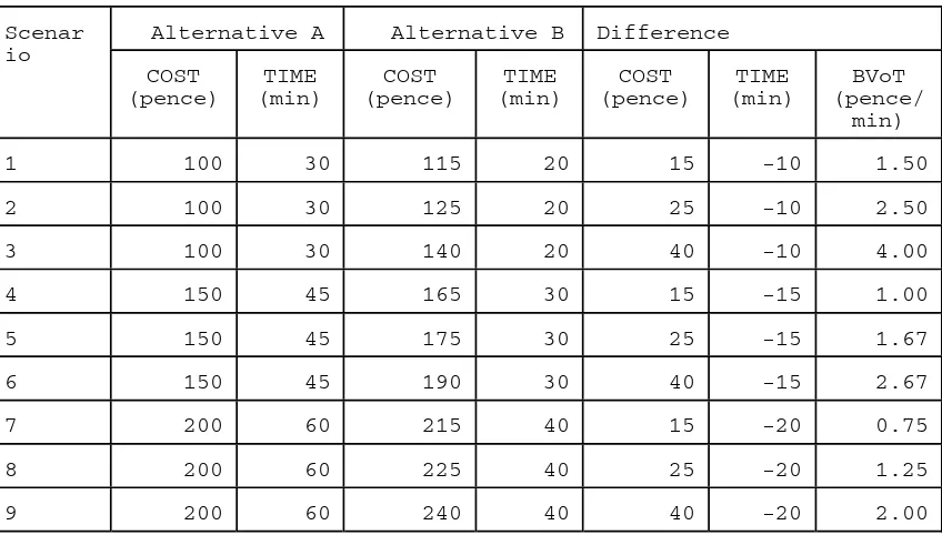
The form of the SP experiments considered here are binary response experiments. Here the

respondent is presented with a small (typically between 9 and 16) number of scenarios. Each scenario

consists of a pair of alternatives (typically, though not necessarily, between two modes), between

which the respondent is invited to choose. Each choice is described by a number of attributes

(typically including cost and time) which are presented as values. A typical two variable SP design,

taken from Fowkes and Nash (1991), is given in table 1.

Alternative A Alternative B Difference

Scenar io

COST (pence)

TIME (min)

COST (pence)

TIME (min)

COST (pence)

TIME (min)

BVoT (pence/

min)

1 100 30 115 20 15 -10 1.50

2 100 30 125 20 25 -10 2.50

3 100 30 140 20 40 -10 4.00

4 150 45 165 30 15 -15 1.00

5 150 45 175 30 25 -15 1.67

6 150 45 190 30 40 -15 2.67

7 200 60 215 40 15 -20 0.75

8 200 60 225 40 25 -20 1.25

[image:6.595.76.500.401.642.2]

9 200 60 240 40 40 -20 2.00

Table 1 : A possible binary choice SP design

In this design, alternative B is always the faster but more expensive option. This need not always be

the case, a mixture of either alternative being the faster, more expensive is acceptable. In fact it is

possible to have one of the alternatives being both the faster and cheaper option.

(7)

express the attributes as the differences in their levels. Thus the question becomes a direct trade-off

between savings in time and cost.

A feature of the design in table 1 is that the correlations between all the attribute differences is zero.

Such a design is said to be orthogonal. This is the first of two widely used design criteria. The

supposed reason for ensuring that this property exists is that this would produce the most efficient

estimates from any model estimation procedure, primarily from an analogy with least squares

regression (Fowkes, 1996).

Another item of information which can be extracted from the design in table 1 are the boundary

values of time (BVoT), ie COST difference divided by TIME difference. These values show at what

time valuation individuals are indifferent between alternatives. Thus for scenario 1, if an individual's

value of time is 1.5 pence per minute then they are indifferent between alternatives A and B in this

scenario. If their value of time is less than 1.5, then they would be expected to choose the slower but

cheaper option (alternative A). If their value of time is greater than 1.5, then alternative B should be

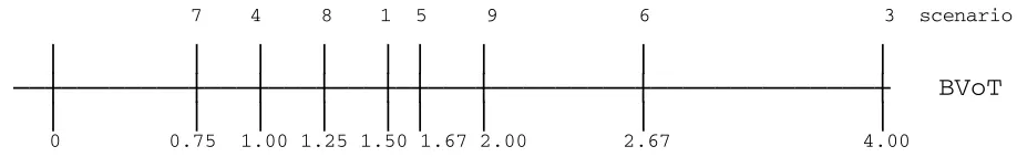
the preferred option. It is possible to plot a graphical representation of the spread of BVoT's. This

plot for the design in table 1 is given in figure 1.

7 4 8 1 5 9 6 3 scenario

BVoT

[image:7.595.66.525.343.414.2]

0 0.75 1.00 1.25 1.50 1.67 2.00 2.67 4.00

Figure 1 : Boundary value map of table 1 design

Figure 1 begins to show how effective a design should be at recovering a range of values of time. In

the discussion which follows a perfect knowledge on the part of the respondent is assumed (ie

deterministic choice). If the respondents are thought to follow compensatory choice processes, some

form of randomness is incorporated into the decision process which represents incorrect (or

inconsistent) choices.

With reference to the example design, if the value of time is greater than 4.00 then all the respondents

will chose the faster, more expensive option. Thus the only clear result will be that the lower bound

of value of time is 4.00. If the value is between 2.67 and 4.00 then all the respondents will chose the

faster, more expensive alternative, except for scenario 3, in which case they would select the slower,

cheaper option. In this case there is both a lower and upper bound on the value of time. The interval

is however wide, at 1.33. If the value of time is between 1.50 and 1.67 then the choice will be the

faster, more expensive mode for scenarios 7, 4, 8 and 1 and the slower, cheaper mode for scenarios 5,

9, 6 and 3. The interval is also narrow at 0.16. Intuitive inspection suggests that this design would

perform well at recovering values of time in the range 1.00 to 2.00.

This methodology is the second design technique which is widely employed in SP design, namely

trying to ensure that there is a reasonable coverage of boundary values near an expected value of

time. There is an extension of this technique into a three variable case, where the boundary points

become boundary rays, with an intercept and a slope (Fowkes 1991).

(8)

which give orthogonality and also give a reasonable coverage of boundary values.

2 MODELLING

Once an SP design has been designed it is used in an experiment to try and extract a valuation of the

measure of interest (in the example given in section 1 it would be the value of time). A model of

individuals behaviour is required from which parameter values can be estimated. An assumption used

here is to derive a set of utilities, for each alternative, which is a linear combination of the attribute

levels. The expression of this utility will be of the form:

ε

β

ε

β

+

TIME

+

COST

=

U

+

TIME

+

COST

=

U

b 2 b 1 b a 2 a 1 a

(1

a)

(1

b

)

An individual will be expected to choose the option which has the highest utility, U

a

or U

b

, depending

on the values for the parameters

1

and

2

. It is also worth noting that most estimation packages do

not directly estimate the

i

's, but instead estimate a scaled

i

ie

i

, where

1

and

2

are the 'true'

i

's.

When estimating values of time (see below) these 's are irrelevant since they cancel out, but if the

estimates are to be used for forecasting purposes then the true underlying

i

's will be required. In

what follows

1

and

2

should be strictly interpreted as

1

and

2

.

The expectations of (1) can be converted into probabilities such that an individual makes their

decision in favour of alternative A if:

0)

>

U

-U

Pr(

=

Pr(a)

)

U

>

U

Pr(

=

Pr(a)

b a b a

(2

a)

(2

b

)

An alternative expression for this choice utility is the utility difference expression:

ε

β

COST

+

TIME

+

=

U

₁

∆

₂

∆

(3

)

Where COST is (COST

b

- COST

a

)

TIME is (TIME

b

- TIME

a

)

Both

1

and

2

are assumed negative since spending extra money or time on a given trip should cause

dis-utility. If U is greater than 0 then the individual prefers alternative A whilst if it is less than 0

then alternative B is the preferred choice. The values of

1

and

2

are usually estimated using

(9)

The probability expression then becomes:

0)

>

U

Pr(

=

Pr(a)

∆

(4

)

Which, under certain assumptions about the distribution of the error terms, can be calculated from:

e

+

1

1 =

Pr(a)

₍ _COST₊ _TIME₎

2

1∆ β ∆

β

(5

)

Thus if this probability is greater than 0.5 then one would assume that the individual will chose

alternative A and otherwise alternative B.

The expression (

2

/

1

) gives a valuation for the overall value of time (VoT).

Expressions can be derived for the variances of the parameters

1

and

2

and the ratio

2

/

1

(Watson

et al, 1996). These expressions involve:

1

,

2

, COST, TIME and additionally in the later

case, Var(

1

), Var(

2

) and Covariance(

1 , 2.

).

3 NEW DESIGN METHODOLOGY

Given an expression for the variance of the parameters, a sensible approach is to derive a design

which, for a given

1

and

2

, chooses COST and TIME to minimise these variances. This is

essentially the new methodology. In reality the values of

1

and

2

will be unknown until the survey is

conducted which is something of a drawback, however, information from pilot or previous full

studies may inform the choice of

1

and

2

, thereby overcoming this drawback.

It has been shown that the adoption of this methodology will produce a design with certain properties

(Wardman and Toner, 1996):

• The Pr(a) = p* which will equal 0.9168 or 0.0832; and

• The t-ratio of the parameters will be given by the expression:

4)

-u

(

2 n

=

t

* 2

(6

)

where u is the utility difference which produces p* in (5), ie ±2.399;

n is the number of scenarios.

In the case under consideration here there are two parameters whose variance can be minimised.

When one variable is at its minimum variance, the other may not be. Thus a number of approaches

suggest themselves:

(1) Successive minimisation of Var(

1

) and Var(

2

);

(2) Successive minimisation of t(

1

) and t(

2

) (minimisation since

1

and

2

are negative) ;

(10)

))

Var(

w

(

i _i

2

=1 i

β

∑

(4) Weighted minimisation of:

|

)

t(betasubi

|

-t

(

w

(

*

i 2

=1 i

∑

Cases (1) and (2) would require iterative minimisation loops, whilst cases (3) and (4) require only

one minimisation. Other minimisation criteria are also possible, eg involving the ratio of t(

i

) to t* or

a weighted sum of the Var(

i

)'s and Var(VoT). Since Var(VoT) is unbounded, however, constraints

may be required here. The results presented in this paper were obtained from FORTRAN programs

which used the NAG (Ford and Pool, 1984) minimisation routine E04JAF. Similar minimisation

routines to perform these tasks can be found in popular spreadsheets.

4 TWO

VARIABLES

4.1 PRODUCING THE DESIGN

The initial design used to illustrate the application of the new methodology is that given in table 1. As

a first step towards the application of this new methodology an exercise was conducted to ensure that

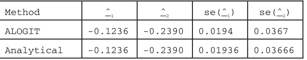
the expressions for the variance parameters were correct. The responses of 20 individuals, with

values of

1

=-0.1 and

2

=-0.2, to the design in table 1 were simulated. The ALOGIT package (1992)

was then used to estimate the _ˆ

1

, _ˆ

2

, se(_ˆ

1

) and se(_ˆ

2

) values from this simulation. These se values are

then compared with the same information from the analytical variance expressions. This comparison

is given in table 2:

Method _ˆ₁ _ˆ₂ se(_ˆ₁) se(_ˆ₂)

ALOGIT -0.1236 -0.2390 0.0194 0.0367

[image:10.595.73.388.494.556.2]

Analytical -0.1236 -0.2390 0.01936 0.03666

Table 2 : Comparison of ALOGIT and analytical expression results

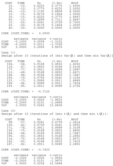
For this section it has been decided to optimise around given values of

1

=-0.1 and

2

=-0.2. The

initial design and the final optimal design for cases (1) and (2) as outlined in section 3, are given in

figure 2. The t* value for a nine scenario design with one individual is 1.9882. The starting point for

both cases is the initial design. Each case has produced a different solution, demonstrating that there

is no unique optimal design. In practice, only integer values of TIME and COST differences are of

use so the final optimal designs are integerised in figure 2. Both cases have produced near p* and t*

values and if non-integer variables are allowed p* values are guaranteed. With the t-ratios only the

last optimised parameter,

2

in this experiment will be at t*. Each t-ratio is based on one replication

of the survey and if many individuals were interviewed then these t-ratios would increase.

(11)

Initial design

COST TIME Pn (1-Pn) BVoT 15. -10. 0.6225 0.3775 1.5000 25. -10. 0.3775 0.6225 2.5000 40. -10. 0.1192 0.8808 4.0000 15. -15. 0.8176 0.1824 1.0000 25. -15. 0.6225 0.3775 1.6667 40. -15. 0.2689 0.7311 2.6667 15. -20. 0.9241 0.0759 0.7500 25. -20. 0.8176 0.1824 1.2500 40. -20. 0.5000 0.5000 2.0000

CORR (COST,TIME) = 0.0000

estimate variance t-ratio COST -0.1000 0.0058 -1.3152 TIME -0.2000 0.0211 -1.3769 VoT 2.0000 0.2926 3.6976

Case (1)

Design after 10 iterations of [min Var( ₁) and then min Var( ₂)]:

CORR (COST,TIME) = -0.7122

Case (2)

Design after 10 iterations of [min t( 1) and then min t( 2)]:

[image:11.595.137.516.137.695.2]

Figure 2 : Initial and final designs for cases (1) and (2)

(12)

stage, 0 is the starting point, 1 is after minimisation of t(

1

), 2 is after minimisation of t(

2

) and 3 is

the final result.

Figure 3 shows that the parameter being optimised

reaches the t* value, whilst the other loses the t* value. As the iterations progress, however, the

extent of this loss deteriorates. The t-ratio for VoT after an initial dip, rises with each iteration. Figure

5 shows the nature of the design at each iteration. The positive line is the maximum cost difference

across all nine scenarios whilst the negative line is the minimum time difference across all nine

scenarios.

A clear saw-tooth pattern is apparent in this figure. A minimisation of t(

1

) increases the maximum

COST difference whilst decreasing the

absolute

value of the TIME difference. A minimisation of

t(

2

) produces the opposite effect. The more iterations, the larger these maximum and minimum

(13)

t(VoT)=5.6758, which is still an improvement on the starting value of t(VoT)=3.6976. The actual

design is provided in figure 6.

[image:13.595.142.410.416.591.2]

Figure 6 : Final Design with 'reasonable' differences

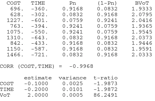
The final designs in cases (3) and (4), with equal weight given to COST and TIME are given in figure

7.

Case (3)

Design after one minimisation of t( i):

(14)

Case (4)

Design after one minimisation of (t*-t( _i))2

:

[image:14.595.143.415.138.314.2]

Figure 7 : Initial and final designs for cases (3) and (4)

Both these cases have quickly produced higher t(VoT) values than those seen for cases (1) and (2).

Case (4) has near p* across all scenarios and t* values for both parameters. The drawback, especially

in case (3), is much higher COST and TIME differences.

4.2 TESTING THE DESIGN

The results in figures 2 and 6 show how well the design performs at recovering values of

1

and

2

around which the design is optimised. The next question is how an optimised design will perform

when recovering other combinations of

1

and

2

? Three situations may arise:

(1)

It is known with a fair degree of confidence the vicinity of the

1

and

2

values;

(2)

It is known with a great deal of confidence a range of

1

and

2

values

(3)

Nothing is known about the location of the

1

and

2

values.

To explore these situations three experiments are conducted. The first is to sample alternative

1

and

2

values in the neighbourhood of the design values, and test them with the design (situation 1). The

second is to use the methodology to try and recovering different combinations of

1

and

2

values

(situation 2). The final experiment is to construct a grid of

1

and

2

values and test the performance

(15)

4.2.1 What's happening in the neighbourhood?

An optimal design is constructed, based on the

second iteration of

2

in case (2).

A large sample of five hundred alternative values of

1

and

2

are randomly sampled from the triangular

distributions in the upper portion of figure 8. These

values produce the distribution of VoT given in the

lower portion of figure 8. Extremes of as large as

5.0 have been allowed. The t-ratios for these 500

alternative values are then calculated on the separate

assumptions of the use of the initial, (orthogonal)

design and the optimal design.

The distribution of the t(

1

), t(

2

) and t(VoT) under

(16)

The optimal design has produced a more uniform distribution of t-ratios for

1

and

2

in comparison

with the more peaked distribution provided by the orthogonal design. The optimal design has

produced fewer small t-ratios and more high t-ratios for t(VoT) than the orthogonal design.

4.2.2 Divide and conquer

Instead of using all nine scenarios to try and recover a fixed combination of

1

and

2

values, it may

be more efficient to partition the scenarios. Thus the first three scenarios could be used to recover

1a

and

2a

, the next three

1b

and

2b

and the last three

1c

and

2c

values. Careful consideration needs to

be given to the approach adopted. Issues worth considering are:

(a)

Should the exercise treat each design as an series of independent mini-SP's? This would

involve an approach similar to that used above but only using the appropriate scenarios

during each optimisation. The scenarios would then be assembled for the full SP.

(b)

Would the allocation of scenarios to

1

and

2

combinations be significant?

(c)

An integrated SP may be required, were the full design is used to calculate the variance

expressions during optimisation (unlike (a) above) but only the relevant scenarios are

changed during optimisation.

(d)

In this case, is the order in which each combination is optimised significant?

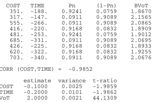
To explore issue (a) the nine scenario design of table 1 is used to recover

1

and

2

values of

(17)

In all but one case (given in italics) this new design has produced an improvement in the t-ratios, and

always an improvement for t(VoT).

The rows labelled Optimal (2) shows the effect of allocating the parameter combinations to different

scenarios (issue b above). Here (-0.1,-0.2) has been allocated to scenarios 4,5 and 6; (-0.1,-0.1) to

scenarios 7,8 and 9 and (-0.1,-0.3) to 1, 2 and 3. Clearly this has an effect since Optimal (1) is

different to Optimal (2) but the improvement over the optimal design is still present.

(

₁

,

₂

)

t(

₁

)

t(

₁

)

t(VoT)

(-0.1,-0.2)

Orthogonal

Optimal (1)

Optimal (2)

-1.3152

-1.3634

-1.3919

-1.3769

-1.3702

-1.3914

3.6976

5.6892

5.7753

(-0.1,-0.1)

Orthogonal

Optimal (1)

Optimal (2)

-1.1956

-1.7896

-1.6186

-0.7963

-1.5661

-1.4278

1.6792

3.5299

3.9043

(-0.1,-0.3)

Orthogonal

Optimal (1)

Optimal (2)

-1.1264

-1.4679

-1.2521

-1.4273

-1.4602

-1.3885

[image:17.595.76.466.213.366.2]

3.0628

4.9610

5.4198

Table 3 : Comparison of Orthogonal and Optimal designs

The alternative approach suggested in (c) above is where the full design is used to calculate the variance

values, but only a subset of the scenarios are allowed to change during optimisation.

The first three scenarios are once again optimised around (-0.1,-0.2) as above, but all nine scenarios are

used to calculate the variances during optimisation. When this stage has been completed the next three

scenarios are used to optimise for (-0.1,-0.1), again changing only these scenarios but using the full design

to calculate the variances. After stage three, where the design is around (-0.1, -0.3) the final design is

complete.

A fuller account of this complex process, with only two iterations, is show in appendix A. Adopting this

approach gives the summary results presented as Optimal (1) in table 4. This approach has produced an

improvement in the t-ratios over the orthogonal design. No consistent pattern emerges when the optimal

results in table 3 are compared with those in table 4.

(18)

(

₁

,

₂

)

t(

₁

)

t(

₁

)

t(VoT)

(-0.1,-0.2)

Orthogonal

Optimal (1)

Optimal (2)

-1.3152

-1.6737

-1.5126

-1.3769

-1.6380

-1.6157

3.6976

4.4300

5.4991

(-0.1,-0.1)

Orthogonal

Optimal (1)

Optimal (2)

-1.1956

-1.6402

-1.3823

-0.7963

-1.7142

-1.4469

1.6792

5.0985

4.6902

(-0.1,-0.3)

Orthogonal

Optimal (1)

Optimal (2)

-1.1264

-1.3555

-1.4544

-1.4273

-1.4075

-1.4500

3.0628

4.9854

6.4594

Table 4 : Comparison of Orthogonal and Optimal integrated designs

4.2.3 The wider picture

An optimal design is constructed, based on the second iteration of

2

in case (2). This design was then

used to calculate a grid of t(VoT) values based on values of

1

and

2

in the range [-0.05,-1.00] in steps of

[image:18.595.71.460.111.262.2]

-0.05. Figure 12 shows the 3D plot for the orthogonal design whilst figure 13 shows the corresponding

plot for the optimal design.

Figure 12 is characterised by a shallow but wide plateau, whilst figure 13 has two sharper, more

concentrated, ridges. Inspection of these two graphs suggests that if the actual

1

and

2

values fall within

either of these two ridges then the optimal design is best, otherwise the orthogonal design may be better.

5 THREE

VARIABLES

The three variable design is a natural extension to that of two variables. Here the utility equations are

given by the expressions:

(19)

A complicating factor is that the construction of point based boundary values are no longer possible. By

way of example consider the SP design given in table 5, taken from a study by Preston and Wardman

(1991).

Alternative A Alternative B

Difference (B-A)

COST (pence)

TIME (min)

DEPART (min)

COST (pence)

TIME (min)

DEPART (min)

COST (pence)

TIME (min)

DEPART (min)

Intercept Slope

1 50 40 0 50 25 30 0 -15 30 0.00 2.0

2 30 45 0 0 25 30 -30 -20 30 -1.50 1.5

3 100 45 0 50 35 30 -50 -10 30 -5.00 3.0

4 75 40 0 0 35 30 -75 -5 30 -15.0 6.0

5 0 40 0 0 35 60 0 -5 60 0.00 12.0

6 80 45 0 50 35 60 -30 -10 60 -3.00 6.0

7 50 45 0 0 25 60 -50 -20 60 -2.50 3.0

8 125 40 0 50 25 60 -75 -15 60 -5.00 4.0

9 50 45 0 50 25 30 0 -20 30 0.00 1.5

10 30 40 0 0 25 30 -30 -15 30 -2.00 2.0

11 100 40 0 50 35 30 -50 -5 30 -10.0 6.0

12 75 45 0 0 35 30 -75 -10 30 -7.50 3.0

13 0 45 0 0 35 60 0 -10 60 0.00 6.0

14 80 40 0 50 35 60 -30 -5 60 -6.00 12.0

15 50 40 0 0 25 60 -50 -15 60 -3.33 4.0

16 125 45 0 50 25 60 -75 -20 60 -3.75 3.0

Table 5 : A possible binary choice three variable SP design

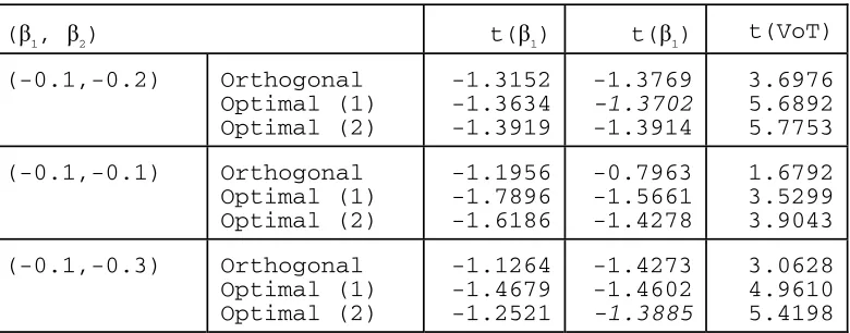
Fowkes (1991) proposes that a boundary ray map may be constructed from this design, where the

intercept and slope of the ray are given by the following expression.

TIME

-DEPARTURE

VoD

+

DELTATIME

-COST

=

BVoT

∆

(8

)

(20)

The units of journey time and departure time change are in single legs of a journey whilst the cost is for a

round trip of two legs. To keep the units consistent the costs have been halved. This map is characterised

by non-positive intercepts with the VoT axis and positive slopes. Note that for the t-ratios, the information

presented is based on only one replication of the survey. The information in figure 14 does not suggest

that the t-ratios of VoT or VoD from the surveys will be as low as 0.5731 or 0.8555

[image:20.595.185.542.111.354.2]

(21)

After only one iteration, the t-ratio of the last optimised parameter ( DEPARTURE) is near its t* value of

2.6510, and the t-ratios of VoT and VoD have shown considerable improvement. The p values are also

close to p*.

During the iterative process the same features as were seen for the two variable case are apparent, namely:

optimised parameter near t; other parameters sub-t but improving; p's at or near p* and increases in the

magnitude of the differences. After ten iterations, the t-ratios for VoT and VoD are high at 11.7439 and

10.5658.

Much of the discussion of section 4.2 with regard to the testing of the design is relevant to a three variable

design. The performance will be good in the neighbourhood of the design point and divide and conquer

approaches are equally applicable to a three variable design. An idea of the wider picture is difficult to

gain since a 4D plot would be required to show the performance of each design at distant points.

6 FOUR

VARIABLES

The application of this methodology to a four variable design begins to show its utility over traditional

approaches for designing SP experiments. Clearly a graphical representation of the design is difficult to

envisage, requiring a 3D plot of graphical planes.

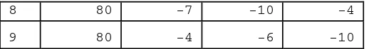
The test design for a binary choice case is shown in table 6. This design is taken from Toner (1991). For

space considerations, only the difference values for the variables are shown.

Fare (pence)

Walk (min)

Wait (min)

IVTime (min)

1 150 -12 -10 -10

2 150 -7 -6 -7

3 150 -4 -3 -4

4 50 -12 -6 -4

5 50 -7 -3 -10

6 50 -4 -10 -7

(22)

8 80 -7 -10 -4

[image:22.595.72.331.110.145.2]

9 80 -4 -6 -10

Table 6 : A possible binary choice four variable SP design (in differences)

(23)

Initial design

COST WALK WAIT IVTIME Pn (1-Pn) 150. -12. -10. -10. 0.1516 0.8484 150. -7. -6. -7. 0.1000 0.9000 150. -4. -3. -4. 0.0718 0.9282 50. -12. -6. -4. 0.4611 0.5389 50. -7. -3. -10. 0.4502 0.5498 50. -4. -10. -7. 0.4693 0.5307 80. -12. -3. -7. 0.3189 0.6811 80. -7. -10. -4. 0.3208 0.6792 80. -4. -6. -10. 0.3165 0.6835 COST WALK WAIT IVTIME

COST 1.0000 0.0000 0.0000 0.0000 WALK 0.0000 1.0000 0.0000 0.0000 WAIT 0.0000 0.0000 1.0000 0.0000 IVTIME 0.0000 0.0000 0.0000 1.0000

estimate t-ratio

Cost -0.0200 -0.8976 * Walk T -0.0340 -0.1778 Wait T -0.0440 -0.1965 IVTime -0.0430 -0.1815 estimate t-ratio

Walk/C 1.7000 0.1878 Wait/C 2.2000 0.2077 Time/C 2.1500 0.1940

Design after min(t( 1)),min(t( 2)),min(t( 3)),min(t( 4))

COST WALK WAIT IVTIME Pn (1-Pn) 144. -81. 16. 36. 0.0849 0.9151 141. -23. -9. 17. 0.0853 0.9147 138. -9. -18. 18. 0.0805 0.9195 91. -303. 69. 182. 0.0847 0.9153 211. 16. 74. -242. 0.9158 0.0842 155. 117. -170. 66. 0.0805 0.9195 377. -211. -25. -39. 0.9177 0.0823 129. 7. -98. -20. 0.9133 0.0867 48. 112. 62. -118. 0.0815 0.9185 COST WALK WAIT IVTIME

COST 1.0000 -0.3459 -0.1527 -0.2405 WALK -0.3459 1.0000 -0.3670 -0.4856 WAIT -0.1527 -0.3670 1.0000 -0.2846 IVTIME -0.2405 -0.4856 -0.2846 1.0000

estimate t-ratio

Cost -0.0200 -1.5593 Walk T -0.0340 -1.6787 Wait T -0.0440 -1.5530 IVTime -0.0430 -1.9880 * estimate t-ratio

(24)

Design after min(t( ₁)),min(t( ₂)),min(t( ₃)),min(t( ₄)) 10 times

COST WALK WAIT IVTIME Pn (1-Pn) 550. -238. -321. 317. 0.0820 0.9180 585. 67. -473. 215. 0.0823 0.9177 350. -61. -387. 337. 0.0840 0.9160 -91. -702. 113. 538. 0.0818 0.9182 1039. 265. 209. -850. 0.0805 0.9195 335. 799. -914. 92. 0.9164 0.0836 1645. -1007. 224. -254. 0.9171 0.0829 516. -12. -147. -136. 0.9171 0.0829 121. 469. 8. -379. 0.0816 0.9184

COST WALK WAIT IVTIME COST 1.0000 -0.3821 0.3581 -0.5315 WALK -0.3821 1.0000 -0.5898 -0.2778 WAIT 0.3581 -0.5898 1.0000 -0.4592 IVTIME -0.5315 -0.2778 -0.4592 1.0000

estimate t-ratio Cost -0.0200 -1.9576 Walk T -0.0340 -1.9609 Wait T -0.0440 -1.9610 IVTime -0.0430 -1.9881 *

[image:24.595.149.450.141.414.2]

estimate t-ratio Walk/C 1.7000 10.6499 Wait/C 2.2000 10.0233 Time/C 2.1500 10.7921

Figure 17 : Initial, first optimised and final designs for table 6

Once again all the features seen for the two variable situation occur here. The p values are close to p*, as

seen previously.

7 TWO VARIABLES PLUS ASC

The equation for the utility of each mode given in (1) can be modified to include an alternative specific

constant (ASC). The role of this constant is to account for factors which are not specifically included in

the design when determining the attractiveness of one mode over another. The revised form of equation

(1) becomes:

ε

β

ε

β

+

TIME

+

COST

=

U

+

TIME

+

COST

+

ASC

=

U

b 2 b 1 b a 2 a 1

a

₍₉

_a)

(9

b

)

If the ASC is estimated to be negative then, all other things being equal, U

a

< U

b

and alternative B would

be preferred over A. If the ASC is positive then A would be the preferred mode. This revised form can be

cast into the general form of an SP by setting one of the variables to a constant value. Table 7 gives an

illustrative example of a two variable design with a range of ASC's, taken from Fowkes (1991).

Alternative A Alternative B Difference (A-B)

(25)

COST (£)

TIME (min)

COST (£)

TIME (min)

COST TIME _{BVoT (pence/min)}

ASC=0 ASC=2 ASC=5

1 40 460 20 260 20.00 240.00 10.00 9.00 7.50

2 60 460 50 260 10.00 250.00 5.00 4.00 2.50

3 60 610 50 210 10.00 200.00 2.50 2.00 1.25

4 40 310 20 210 20.00 190.00 20.00 18.00 15.00

5 60 460 20 360 40.00 320.00 40.00 38.00 35.00

6 40 310 50 360 -10.00 370.00 20.00 24.00 30.00

Table 7 : Two variable with an ASC design

[image:25.595.141.456.379.749.2]

If there is an expectation that the ASC is zero then the methodology used in section 4 can be applied.

Otherwise the optimisation process must take account of the presence of the ASC but must not alter its

value since it is, like

1

and

2

, a given parameter.

Figure 18 shows the results after 15 iterations of min(t(

1

)) and min(t(

2

)) with ASC's of 2.00 and 5.00.

Initial design with ASC=2.00

ASC COST TIME Pn (1-Pn) BVoT 2. 20. -200. 0.0573 0.9427 0.0900 2. 10. -200. 0.5498 0.4502 0.0400 2. 10. -400. 0.8022 0.1978 0.0200 2. 20. -100. 0.0323 0.9677 0.1800 2. 40. -100. 0.0001 0.9999 0.3800 2. -10. 50. 0.9910 0.0090 0.2400

ASC 2.00000 6.63744 0.77630 COST -0.30000 0.08949 -1.00285 TIME -0.00600 0.00017 -0.45634 T/C 0.02000 15450.01465 0.00016

Design after 10 iterations

ASC COST TIME Pn (1-Pn) BVoT 2. 178. -214. 0.0000 1.0000 0.8224 2. 5. -283. 0.9001 0.0999 0.0106 2. 19. -977. 0.8968 0.1032 0.0174 2. 19. -160. 0.0607 0.9393 0.1062 2. 18. -128. 0.0671 0.9329 0.1250 2. -1. 814. 0.0702 0.9298 0.0037

ASC 2.00000 2.70369 1.21633 COST -0.30000 0.08331 -1.03938 TIME -0.00600 0.00002 -1.46319 T/C 0.02000 1111.05481 0.00060

Initial design with ASC=5.00

(26)

5. 10. -200. 0.9608 0.0392 0.0250 5. 10. -400. 0.9879 0.0121 0.0125 5. 20. -100. 0.4013 0.5987 0.1500 5. 40. -100. 0.0017 0.9983 0.3500 5. -10. 50. 0.9995 0.0005 0.3000

ASC 5.00000 4.88852 2.26142 COST -0.30000 0.21312 -0.64985 TIME -0.00600 0.00059 -0.24766 T/C 0.02000 59243.35547 0.00008

Design after 10 iterations

ASC COST TIME Pn (1-Pn) BVoT 5. 193. -178. 0.0000 1.0000 1.0562 5. 12. -163. 0.9151 0.0849 0.0429 5. 28. -958. 0.9128 0.0872 0.0240 5. -82. -121. 1.0000 0.0000 -0.7190 5. 24. 20. 0.0895 0.9105 -0.9500 5. 15. 461. 0.0940 0.9060 -0.0217

[image:26.595.148.450.109.403.2]

ASC 5.00000 1.93686 3.59270 COST -0.30000 0.13150 -0.82730 TIME -0.00600 0.00002 -1.32280 T/C 0.02000 2065.62158 0.00044

Figure 18 : Initial and final designs for ASC=2.00 and ASC=5.00.

In both cases the final design has produced improvements in the t-ratios for all parameters. For the case

where ASC=2.00, the final optimised design does not possess p* values, the first time this feature has

been noted. When ASC=5.00 the design does contains some near p* but also some 1.0 or 0.0 p's. The

final t(

2

) value in this design, 1.32280 corresponds to a t*=1.32548 with n=4, ie the number of scenarios

with p*'s.

8 CONSTRAINTS

One undesirable feature of this methodology is the tendency to produce large magnitude differences in the

variables. This may be practically impossible or infeasible. One approach is to set limits on these

differences. The optimisation process can either be stopped when any of these limits are exceeded or

constrained to operate within these limits. The first approach was adopted in section 4 where the design

after only two iterations was chosen as the best. This design still gave a reasonable increase in all the

t-ratio's over the initial design. The second approach is to specify constraints in the optimisation process.

By way of example, the COST variable can be constrained to lie within [1,100] and the TIME to be

within [-50,-1]. When this modification is applied, the results are as given in figure 19.

Initial design (as given in figure 2)

(27)

15. -15. 0.8176 0.1824 1.0000 25. -15. 0.6225 0.3775 1.6667 40. -15. 0.2689 0.7311 2.6667 15. -20. 0.9241 0.0759 0.7500 25. -20. 0.8176 0.1824 1.2500 40. -20. 0.5000 0.5000 2.0000

estimate variance t-ratio

COST -0.1000 0.0058 -1.3152 TIME -0.2000 0.0211 -1.3769 VoT 2.0000 0.2926 3.6976

Final design after 10 iterations of min(t( 1)) and min(t( 2))

COST -0.1000 0.0027 -1.9123 TIME -0.2000 0.0101 -1.9871 VoT 2.0000 0.0806 7.0445

Final design after 1 iteration of (t*-t( _i))2

[image:27.595.137.470.95.647.2]

COST -0.1000 0.0026 -1.9595 TIME -0.2000 0.0103 -1.9721 VoT 2.0000 0.0889 6.7096

Figure 19 : Constrained two variable design

(28)

9 CONCLUSIONS

This paper has demonstrated that the methodology devised can be applied to practical binary choice

Stated Preference designs. To summarise, the methodology is:

• simple in its application;

• able to deliver real, quantifiable benefits over traditional SP design methodologies;

• is applicable to an n-variable design, n>2;

• can accommodate designs with alternative specific constants;

• flexible enough to code an incorporate a variety of user requirements;

• works within constraints;

• simple to implement in spreadsheets or FORTRAN code.

REFERENCES

Hague Consulting Group (1992). "ALOGIT Users' Guide, version 3.2".

Ford, B and Pool, JCT (1984). "The Evolving NAG Library Service. Sources and Development of

Mathematical Software."

Prentice-Hall

, pp375-397.

Fowkes, AS (1991). "Recent developments in Stated Preference techniques in transport research".

PTRC-SAM, Sussex 1991, published as

Transportation Planning Methods

, Code P347, pp.251-263, PTRC,

London

Fowkes, AS (1996). "The development of Stated Preference Techniques in Transport Planning".

ITS

Working Paper 479

, Institute for Transport Studies, University of Leeds, Leeds.

Fowkes, AS and Nash, CA (eds) (1991). "Analysing Demand for Rail Travel".

Avebury Publishing

Group

, Chapter 4, pp33-56.

Fowkes, AS and Wardman, M (1993). "Non-orthogonal Stated Preference design". PTRC-SAM, UMIST

1993, published as

Transportation Planning Methods

, Code P366, pp.91-97, PTRC, London

Toner, JP (1991). "The economics of regulation of the taxi trade in British towns".

Unpublished PhD

Thesis

, University of Leeds, Leeds, UK.

Preston, J and Wardman, M (1991). "The use of hypothetical questioning techniques to assess the future

demand for travel in the Nottingham area".

UTSG 23rd Annual Conference, University of Nottingham.

Wardman, M and Toner, JP (1996). "Issues in Model Specification".

Paper to PTRC Conference on Value

of Time

, London, October 1996.

(29)

APPENDIX

Non-integrated

The three parameter pairs (-0.1,-0.2), (-0.1,-0.1) and (-0.1,-0.3) with the initial design

COST -0.1000 0.0058 -1.3152 TIME -0.2000 0.0211 -1.3769 VoT 2.0000 0.2926 3.6976

(30)

Optimise (-0.1,-0.2)

COST TIME Pn (1-Pn) BVoT 61. -42. 0.9089 0.0911 1.4524 22. 1. 0.0832 0.9168 -22.0000 38. -7. 0.0832 0.9168 5.4286

COST TIME Pn (1-Pn) BVoT 90. -57. 0.9168 0.0832 1.5789 33. -4. 0.0759 0.9241 8.2500 57. -17. 0.0911 0.9089 3.3529

COST TIME Pn (1-Pn) BVoT 59. -83. 0.9168 0.0832 0.7108 24. 1. 0.0759 0.9241 -24.0000 35. -11. 0.0832 0.9168 3.1818

(31)

All three segments are assembled to give the final design and the t-ratios are calculated.

(32)

Integrated

The starting designs are the same as those for the non-integrated process

COST TIME Pn (1-Pn) BVoT

104. -64. 0.9168 0.0832 1.6250 Only change

47. -11. 0.0759 0.9241 4.2727 these three

94. -35. 0.0832 0.9168 2.6857 scenarios

15. -15. 0.8176 0.1824 1.0000 25. -15. 0.6225 0.3775 1.6667 40. -15. 0.2689 0.7311 2.6667 15. -20. 0.9241 0.0759 0.7500 25. -20. 0.8176 0.1824 1.2500 40. -20. 0.5000 0.5000 2.0000

163. -187. 0.9168 0.0832 0.8717 Only change

5. 19. 0.0832 0.9168 -0.2632 these three

34. -10. 0.0832 0.9168 3.4000 scenarios

15. -20. 0.6225 0.3775 0.7500 25. -20. 0.3775 0.6225 1.2500 40. -20. 0.1192 0.8808 2.0000

COST TIME Pn (1-Pn) BVoT 104. -64. 0.9998 0.0002 1.6250 47. -11. 0.1978 0.8022 4.2727 94. -35. 0.7503 0.2497 2.6857 163. -187. 1.0000 0.0000 0.8717 5. 19. 0.0020 0.9980 -0.2632 34. -10. 0.4013 0.5987 3.4000

-42. 6. 0.9168 0.0832 7.0000 Only change

-16. -3. 0.9241 0.0759 -5.3333 these three

26. -17. 0.9241 0.0759 1.5294 scenarios

(33)

The three parameter pairs with optimal design

COST TIME Pn (1-Pn) BVoT 104. -64. 0.9168 0.0832 1.6250 47. -11. 0.0759 0.9241 4.2727 94. -35. 0.0832 0.9168 2.6857 163. -187. 1.0000 0.0000 0.8717 5. 19. 0.0134 0.9866 -0.2632 34. -10. 0.1978 0.8022 3.4000 -42. 6. 0.9526 0.0474 7.0000 -16. -3. 0.9002 0.0998 -5.3333 26. -17. 0.6900 0.3100 1.5294

(34)

Change the sequence of parameter pairs

COST TIME Pn (1-Pn) BVoT 15. -10. 0.8176 0.1824 1.5000 25. -10. 0.6225 0.3775 2.5000 40. -10. 0.2689 0.7311 4.0000 15. -15. 0.9526 0.0474 1.0000 25. -15. 0.8808 0.1192 1.6667 40. -15. 0.6225 0.3775 2.6667

-145. 40. 0.9241 0.0759 3.6250 Only change

-71. 16. 0.9089 0.0911 4.4375 these three

-159. 61. 0.0832 0.9168 2.6066 scenarios

COST TIME Pn (1-Pn) BVoT

140. -82. 0.9168 0.0832 1.7073 Only change

-9. 16. 0.0911 0.9089 0.5625 these three

28. -2. 0.0832 0.9168 14.0000 scenarios

15. -15. 0.8176 0.1824 1.0000 25. -15. 0.6225 0.3775 1.6667 40. -15. 0.2689 0.7311 2.6667 -145. 40. 0.9985 0.0015 3.6250 -71. 16. 0.9802 0.0198 4.4375 -159. 61. 0.9759 0.0241 2.6066

COST TIME Pn (1-Pn) BVoT 140. -82. 0.0030 0.9970 1.7073 -9. 16. 0.3318 0.6682 0.5625 28. -2. 0.0691 0.9309 14.0000

145. -169. 0.9168 0.0832 0.8580 Only change

37. -13. 0.0832 0.9168 2.8462 these three

67. -43. 0.0832 0.9168 1.5581 scenarios

-145. 40. 1.0000 0.0000 3.6250 -71. 16. 0.9959 0.0041 4.4375 -159. 61. 0.9999 0.0001 2.6066

(35)

The three parameter pairs with optimal design

COST TIME Pn (1-Pn) BVoT 140. -82. 1.0000 0.0000 1.7073 -9. 16. 0.0198 0.9802 0.5625 28. -2. 0.0998 0.9002 14.0000 145. -169. 1.0000 0.0000 0.8580 37. -13. 0.5498 0.4502 2.8462 67. -43. 0.9980 0.0020 1.5581 -145. 40. 0.9241 0.0759 3.6250 -71. 16. 0.9089 0.0911 4.4375 -159. 61. 0.0832 0.9168 2.6066

Application of Advanced Stated Preference Design Methodology

White Rose Research Online URL for this paper:

http://eprints.whiterose.ac.uk/2109/

Monograph:

Clark, S.D. and Toner, J.P. (1997) Application of Advanced Stated Preference Design

Methodology. Working Paper. Institute of Transport Studies, University of Leeds , Leeds,

UK.

Working Paper 485

White Rose Research Online

http://eprints.whiterose.ac.uk/

Institute of Transport Studies

University of Leeds

This is an ITS Working Paper produced and published by the University of

Leeds. ITS Working Papers are intended to provide information and encourage

discussion on a topic in advance of formal publication. They represent only the

views of the authors, and do not necessarily reflect the views or approval of the

sponsors.

White Rose Repository URL for this paper:

http://eprints.whiterose.ac.uk/

2109

Published paper

Stephen Clark and Jeremy Toner (1997)

Application of Advanced Stated

Preference Design Methodology.

Institute of Transport Studies, University of

Leeds, Working Paper 485

EPSRC Research Working Paper

APPLICATION OF ADVANCED STATED PREFERENCE DESIGN

METHODOLOGY

Stephen Clark and Jeremy Toner

Document Control Information

Title

: APPLICATION OF ADVANCED STATED PREFERENCE DESIGN

METHODOLOGY

Authors

:

Stephen Clark and Jeremy Toner

Reference Number

:

9612/01

Version

:

1.0

Date

: 14

February

1997

Distribution

:

Availability

:

Unrestricted

File

:

E:\HOME\SP\WP485.WP6

Authorised by

:

Stephen Clark

ITS Working Paper 485

ISSN 0142-8942

December 1996

APPLICATION OF ADVANCED STATED PREFERENCE

DESIGN METHODOLOGY

SD Clark

JP Toner

This work was undertaken on a project sponsored by the Engineering and Physical Sciences

esearch Council (Grant Ref: GR/J81242)

R

CONTENTS

ABSTRACT... 1

1 BACKGROUND ... 1

2 MODELLING ... 3

3

NEW DESIGN METHODOLOGY ... 4

4 TWO

VARIABLES... 5

4.1

PRODUCING THE DESIGN ... 5

4.2

TESTING THE DESIGN... 9