This is a repository copy of The theory of classification part 2: the scratch-built typechecker.
White Rose Research Online URL for this paper: http://eprints.whiterose.ac.uk/79276/
Version: Published Version
Article:
Simons, A.J.H. (2002) The theory of classification part 2: the scratch-built typechecker. Journal of Object Technology, 1 (2). 47 - 54. ISSN 1660-1769
[email protected] https://eprints.whiterose.ac.uk/
Reuse
Unless indicated otherwise, fulltext items are protected by copyright with all rights reserved. The copyright exception in section 29 of the Copyright, Designs and Patents Act 1988 allows the making of a single copy solely for the purpose of non-commercial research or private study within the limits of fair dealing. The publisher or other rights-holder may allow further reproduction and re-use of this version - refer to the White Rose Research Online record for this item. Where records identify the publisher as the copyright holder, users can verify any specific terms of use on the publisher’s website.
Takedown
If you consider content in White Rose Research Online to be in breach of UK law, please notify us by
Vol. 1, No. 2, July-August 2002
The Theory of Classification
Part 2: The Scratch-Built Typechecker
Anthny J. H. Simons, Depdpartment of Computer Science, University of Sheffield, UK
1 INTRODUCTION
This is the second article in a regular series on object-oriented type theory, aimed specifically at non-theoreticians. Eventually, we aim to explain the behaviour of languages such as Smalltalk, C++, Eiffel and Java in a consistent framework, modelling features such as classes, inheritance, polymorphism, message passing, method combination and templates or generic parameters. Along the way, we shall look at some important theoretical approaches, such as subtyping, F-bounds, matching and the object calculus. Our goal is to find a mathematical model that can describe the features of these languages; and a proof technique that will let us reason about the model. This will be the "Theory of Classification" of the series title.
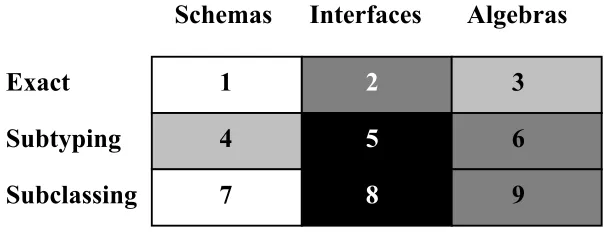
Exact
Subtyping
Subclassing
Schemas Interfaces Algebras
1 2
5
8
4
7
3
6
[image:2.612.123.427.470.586.2]9
Figure 1: Dimensions of Type Checking
THE THEORY OF CLASSIFICATION – PART 2: THE SCRATCH-BUILT TYPECHECKER
48 JOURNAL OF OBJECT TECHNOLOGY VOL.1,NO.2
was expected. Combining these two dimensions, there are up to nine combinations to consider, as illustrated in figure 1. However, we shall be mostly interested in the darker shaded areas. In this second article, we shall build a typechecker that can determine the exact syntactic type (box 2, in figure 1) of expressions involving objects encoded as simple records.
2 THE
UNIVERSE
OF
VALUES AND TYPES
Rather like scratch-building a model sailing ship out of matchsticks, all mathematical model-building approaches start from first principles. To help get off the ground, most make some basic assumptions about the universe of values. Primitive sets, such as
Boolean, Natural and Integer are assumed to exist (although we could go back further and construct them from first principles, in the same way as we did the Ordinal type [1]; this is quite a fascinating exercise in the λ-calculus [2]). All other kinds of concept have to be defined using rules to say how the concept is formed, and how it is used. We shall assume that there are:
• sets A, B, ..., corresponding to the given primitive types in the universe; and • elements a, b, ..., of these sets, corresponding to the values in the universe; and • set operations such as membership ∈, inclusion ⊆, and union ∪; and
• logical operations such as implication ⇒, equivalence ⇔ and entailment
With this starter-kit, we can determine whether a value belongs to a type, since: x : X ("x is of type X") can be interpreted as x ∈ X in the model; or whether two types are related, for example: Y <: X ("Y is a subtype of X") can be interpreted as the subset relationship Y ⊆ X in the model [3].
3 RULES FOR PAIRS
An immediately useful construction which we do not yet have is the notion of a pair of values, 〈n, m〉, possibly taken from different types N and M. The type of pairs is known as a product type, or Cartesian product, since there are N × M possible parings of elements n ∈ N, and m ∈ M. Formally, we require a rule to introduce the syntax for a product type. This is called a type introduction rule. In its simplest form (ignoring the notion of context, which is roughly the same idea as variable scope), the rule for forming a product is:
n : N, m : M
[Product Introduction]
This rule is expressed in the usual style of natural deduction, with the premises above the line and the conclusions below. In longhand, it says "if n is of type N and m is of type M, then we may conclude that a pair 〈n, m〉 has the product type N × M". The rule introduces the syntax for writing pair-values and pair-types, but also defines the relationship between the values and the types (the order of the values n and m determines the structure of the type N × M).
For pair constructions to be useful, we need to know how to access the elements of a pair, and determine their types. We define the first and second projections of a pair, usually written in the style: π1(e), π2(e) applied to some pair-value e. The projections are defined formally in an elimination rule, so called because it deconstructs the pair to access its elements:
e : N × M
[Product Elimination]
π1(e) : N, π2(e) : M
"If e is a pair of the product type N × M, then the first projection π1(e) has the type N, and the second projection π2(e) has the type M." Note that, in this rule, e is presented as a single expression-variable, but we know it stands for a pair from its type N × M. In both rules, the horizontal line has the force of an implication, which we could also write using
⇒.
4 RULES FOR FUNCTIONS
Consider an infinite set of pairs: {〈1, false〉, 〈2, true〉, 〈3, false〉, 〈4, true〉, 〈5, false〉...}. This set is an enumeration of a relationship between Natural numbers and Boolean values - it is in fact one possible representation of the function even(). Since functions have this clear, natural interpretation in our model, we are justified in introducing a special syntax for them:
x : D e : C
[Function Introduction]
λx.e : D → C
"If variable x has the type D and, as a consequence, expression e has the type C, we may conclude that a function of x with body e has the function type D → C." This rule introduces the λ-syntax for functions and the arrow-syntax for function types. If you happen to be a hellenophobic1 engineer, simply consider that: λx.e ⇔ f(x) = e. The type
1
THE THEORY OF CLASSIFICATION – PART 2: THE SCRATCH-BUILT TYPECHECKER
50 JOURNAL OF OBJECT TECHNOLOGY VOL.1,NO.2
signature for a function is always written as an arrow type D → C, with the function's
domain (input set) D on the left and the codomain (output set) C on the right. The
premise of this rule relates the required types of x : D, e : C using entailment , since the type of the body expression e : C is not independent, but "follows from" the type of the variable x : D. This is because the body expression will contain occurrences of x, the variable. Consider that a function may return its argument - in that case, the result type is
the argument type; there is clearly a dependency.
The function elimination rule explains the type of an expression involving a function application. In so doing, it also defines the parenthesis syntax for function application:
f : D → C, v : D
[Function Elimination]
f(v) : C
"If f is a function from D → C, and v is a value of type D, then the result of the function application f(v) is of type C". This rule also expresses the notion of type-sound function application: it allows f to be applied only to values of the domain type D (technically, the rule allows you to deduce that the result of function application is well-typed in this circumstance, but is otherwise undefined).
Do we need rules for multi-argument functions? Not really, because we already have the separate product rules. The domain D in the function rules could correspond, if we so wished, to a type that was a product: D ⇔ N × M. In this case, the argument value would in fact be a pair v : N × M. We assume that any single type variable in one rule can be matched against a constructed type in another rule, if we so desire.
5 RULES FOR RECORDS
Most model encodings for objects [4, 5, 6] treat them as some kind of record with a number of labelled fields, each storing a differently-typed value. So far, we do not have a construction for records in our model. However, consider that a record is rather like a finite set of pairs, relating labels to values: {〈name, "John"〉, 〈surname, "Doe"〉, 〈age, 25〉, 〈married, false〉}. Since a record has this clear, natural interpretation in the model, we are justified in introducing a special syntax. If A is the primitive type of labels:
αi : A, ei : Ti
for i = 1..n [Record
{α1 a e1, ..., αn a en} : {α1 : T1, ..., αn : Tn} Introduction]
constructed by pairing the ith label with the corresponding ith type". This rule uses the index i to link corresponding labels, values and types. In the conclusion, the set-braces are used for records and record types deliberately, since these are sets of pairs. The label-to-value pairings are notated as mappings αia ei, for visual clarity and convenience.
The corresponding record elimination rule introduces the dot or record selection
operator, defining how to deconstruct a record to select a field and then determine its type:
e : {α1 : T1, ..., αn : Tn}
for i = 1..n [Record Elimination]
e.αi : Ti,
"If e has the type of a record, with n labels αi, mapping to types Ti, then the result of selecting the ith field e.αi has the ith type Ti."
6 APPLYING THE RULES
We have a set of rules for constructing pairs, functions and records. With this, we can model simple objects as records. Ignoring the issue of encapsulation for the moment, a simple Cartesian point object may be modelled as a record whose field labels map to simple values (attributes) and to functions (methods). We require a function for constructing points:
make-point : Integer × Integer → Point
This is a type declaration, stating that make-point is a function that accepts a pair of Integers and returns a Point type (which is so far undefined). The full definition of make-point:
make-point = λ(e : Integer × Integer) .
{ x aπ1(e), y aπ2(e), equal aλ(p : Point).(π1(e) = p.x ∧π2(e) = p.y) }
names the argument expression e supplied upon creation and returns a record having the fields x, y and equal. The x and y fields map to simple values, projections of e; the equal
THE THEORY OF CLASSIFICATION – PART 2: THE SCRATCH-BUILT TYPECHECKER
52 JOURNAL OF OBJECT TECHNOLOGY VOL.1,NO.2
fields. Finally, even make-point is properly constructed using the function introduction
rule, with Integer × Integer as the domain type and Point as the codomain type.
The rules permit us to deduce that objects can be constructed using make-point, and also that they are well-typed. Let us now construct some points and expressions involving points, to see if these are well-typed. The let ... in syntax is a way of introducing a scope for the values p1 and p2, in which the following expressions are evaluated:
let p1 = make-point(3, 5) in
p1.x;
Is p1.x meaningful, and does it have a type? The record elimination rule says this is so, provided p1 is an instance of a suitable record type. Working backwards, p1 must be a record with at least the type: {... x : X ... } for some type X. Working forwards, p1 was constructed using make-point, so we know it has the Point type, which, when expanded, is equivalent to the record type: { x : Integer, y : Integer, equal : Point → Boolean }, which also has a field x : Integer. Matching up the two, we can deduce that p1.x : Integer.
let p1 = make-point(3, 5), p2 = make-point(3, 7) in
p1.equal(p2);
Is p1.equal(p2) meaningful, and does it have a type? Again, by working backwards through the record elimination rule, we infer that p1 must have at least the type {... equal : Y ...} for some type Y. Working forwards, we see that p1 has a field equal : Point → Boolean, so by matching up these, we know Y ⇔ Point → Boolean. So, the result of selecting p1.equal is a function expecting another Point. Let us refer to this function as f. In the rest of the expression, f is applied to p2, but is this type correct? Working forwards, p2 was defined using make-point, so has the type Point. Working backwards through the function elimination rule, the function application f(p2) is only type-sound if f has the type Point → Z, for some type Z. From above, we know that f : Point → Boolean, so by matching Z ⇔ Boolean, we confirm that the expression is well-typed and also can infer the expression's result type: p1.equal(p2) : Boolean.
7 CONCLUSION
and records, are formed and under what conditions they are well-typed; elimination rules describe how these constructions may be decomposed into their simpler elements, and what types these parts have. Both kinds of rule were used in a typechecker, which was able to determine the syntactic correctness of method invocations. The formal style of reasoning, chaining both forwards and backwards through the ruleset, was illustrated. The simple model still has a number of drawbacks: there is no updating or encapsulation of state; there are problems looming to do with recursive definitions; and we ignored the context (scope) in which the definitions take effect. In the next article, we shall examine some different object encodings that address some of these issues.
REFERENCES
[1] A J H Simons, Perspectives on type compatibility, Journal of Object Technology 1(1), May, 2002.
[2] A J H Simons, Appendix 1 : λ-Calculus, in: A Language with Class: the Theory of Classification Exemplified in an Object-Oriented Language, PhD Thesis,
University of Sheffield, 1995, 220-238. See http://www.dcs.shef.ac.uk/~ajhs/classify/.
[3] L Cardelli and P Wegner, On understanding types, data abstraction and polymorphism, ACM Computing Surveys, 17(4), 1985, 471-521.
[4] J C Reynolds, User defined types and procedural data structures as
complementary approaches to data abstraction, in: Programming Methodology: a Collection of Articles by IFIP WG2.3, ed. D Gries, 1975, 309-317; reprinted from New Advances in Algorithmic Languages, ed. S A Schuman, INRIA, 1975, 157-168.
[5] W Cook, Object-oriented programming versus abstract data types, in:
Foundations of Object-Oriented Languages, LNCS 489, eds. J de Bakker et al., Springer Verlag, 1991, 151-178.
THE THEORY OF CLASSIFICATION – PART 2: THE SCRATCH-BUILT TYPECHECKER
54 JOURNAL OF OBJECT TECHNOLOGY VOL.1,NO.2
About the author