Doubly Dynamic Equilibrium Distribution Approximation Model for Dynamic Traffic Assignment

(1)

This is a repository copy of Doubly Dynamic Equilibrium Distribution Approximation Model

for Dynamic Traffic Assignment.

White Rose Research Online URL for this paper:

http://eprints.whiterose.ac.uk/84680/

Version: Accepted Version

Book Section:

Balijepalli, NC orcid.org/0000-0002-8159-1513 and Watling, DP

orcid.org/0000-0002-6193-9121 (2005) Doubly Dynamic Equilibrium Distribution

Approximation Model for Dynamic Traffic Assignment. In: Mahmassani, HS, (ed.)

Transportation and Traffic Theory: Flow, Dynamics and Human Interaction - Proceedings

of the 16th International Symposium on Transportation and Traffic Theory. Emerald Group

Publishing Limited , Bingley, UK , pp. 741-760. ISBN 9780080446806

© 2005 Emerald Group Publishing Limited. This is an author produced version of a paper

published in Transportation and Traffic Theory: Flow, Dynamics and Human Interaction -

Proceedings of the 16th International Symposium on Transportation and Traffic Theory.

Uploaded in accordance with the publisher's self-archiving policy.

eprints@whiterose.ac.uk https://eprints.whiterose.ac.uk/

Reuse

Unless indicated otherwise, fulltext items are protected by copyright with all rights reserved. The copyright exception in section 29 of the Copyright, Designs and Patents Act 1988 allows the making of a single copy solely for the purpose of non-commercial research or private study within the limits of fair dealing. The publisher or other rights-holder may allow further reproduction and re-use of this version - refer to the White Rose Research Online record for this item. Where records identify the publisher as the copyright holder, users can verify any specific terms of use on the publisher’s website.

Takedown

If you consider content in White Rose Research Online to be in breach of UK law, please notify us by

(2)

Equilibrium distribution approximation model 1

DOUBLY DYNAMIC EQUILIBRIUM

DISTRIBUTION APPROXIMATION MODEL

FOR DYNAMIC TRAFFIC ASSIGNMENT

N.C.Balijepalli and D.P.Watling, Institute for Transport Studies, University of Leeds, Leeds, England

ABSTRACT

The paper presents research aimed at unifying the fields of (i) dynamic network equilibrium, (ii) dynamic whole-link models and (iii) stochastic process models of between- and within-day dynamics. An approximation result and computational procedure is derived for determining the equilibrium probability distribution of a within- and between-day dynamic stochastic process traffic assignment model. The method is based on an analytic procedure requiring only knowledge of within-day dynamic stochastic user equilibrium flows, together with the Jacobians of the dynamic network loading map and of the choice probability function. An implementation is reported with a particular form of whole-link, continuous-time, dynamic network loading model, commonly found in the literature on dynamic traffic assignment, where travel times at the time of entry to a link are a function of the number of vehicles on the link at that time. Illustrative numerical examples are presented.

INTRODUCTION

(3)

2 Insert book title here

have been identified in established network equilibrium theory in being able to reflect the impacts of such systems, two particular features have attracted much attention. These are namely:

- the representation of dynamic traffic flow phenomena and their impact on departure-time-dependent route choice (“within-day dynamics”); and

- the representation of behavioural adaptation, learning and information acquisition processes (“between-day dynamics”).

A range of techniques has been proposed to address each of these limitations, yet two broad philosophical approaches have been adopted. The first stream of work is based on the attempt to generalise existing network equilibrium theory to the within-day dynamic case, utilising formulations and solution methods from optimal control theory, variational inequalities and mathematical programming. Such a stream provides a range of potentially efficient solution methods, which can be applied and monitored in a well-controlled environment, based on an explicit and well-researched theoretical principle. This theory allows properties of existence and uniqueness of the model prediction and convergence of solution algorithms to be established, and to be linked to the specific assumptions of the underlying model. The second stream is based on an explicit representation of the emergent dynamical processes involved, rather than a direct characterisation of some stationary/equilibrium state of the process. When implemented using an explicit simulation of the system dynamics, this stream of work provides the opportunity to model behaviours that are well beyond those permitted in the well-controlled environment of equilibrium theory, yet without reference to a well-researched theoretical principle describing the system trajectory, and without the control on model outputs one can exert within an equilibrium framework. The price paid for the flexibility of this approach is the greatly added complexity in interpretation of model outputs (as well as in their use for an overall economic evaluation), with predictions that may be transient, stochastic, chaotic, periodic, auto-correlated and depend on the initial conditions. Thus, each of the two streams offers its own advantages, but has its drawbacks.

In the present paper, we shall present research that for the first time unifies the advantages of these competing philosophies, by bringing together three elements, namely:

- the representation of both within- and between-day dynamics within the overall framework of a discrete-time stochastic process, as proposed in the unifying framework of Cantarella and Cascetta (1995);

- the representation of within-day traffic flow dynamics by a continuous-time, whole-link, dynamic network loading model of the kind popularly used in the dynamic traffic assignment literature; and

- the solution and estimation of the equilibrium properties of the resulting stochastic process using a combination of conventional within-day dynamic network equilibrium theory and a theoretical approximation result.

(4)

within a common theoretical framework, whereby advances in one area may be used to the advantage of other areas.

Specifically, the modelling approach adopted is based on modelling the day-by-day evolution of driver decisions as a discrete-time markov process, and the evolution of traffic flow dynamics within the day by a continuous-time whole-link model (hence it is termed ‘doubly dynamic’). While it is known that the stationary output of such a model, in the form of an equilibrium probability distribution of time-dependent network flows, may in principle be estimated by Monte Carlo simulation, there are many potential drawbacks of such an approach, such as the difficulties of detecting stationarity and the effects of multiple attractors, and of dealing with Monte Carlo error in policy tests (Cantarella & Cascetta, 1995; Watling, 1996; Watling, 2002).

With such considerations in mind, Hazelton & Watling (2004) proposed an analytic approximation method for directly estimating the equilibrium probability distribution of such a model, without the need for simulation, and requiring only knowledge of a conventional Stochastic User Equilibrium (SUE) solution. Utilising a result previous established by Davis and Nihan (1993), namely that this equilibrium distribution is asymptotically multivariate normal, with mean the SUE flow vector, then all that is required to complete the approximation process is the variance-covariance matrix of the flows, as provided by the approximation result of Hazelton and Watling (2004). However, a significant restriction of their work is that it was restricted to within-day static models. The contribution of the present paper is to make the important step of extending this work to the within-day dynamic case, in which the origin-destination demand flows are time-sliced by departure time (to any desired resolution), and in which the interactions on the network are handled through a continuous-time, dynamic network loading model (estimated in practice by an arbitrarily fine discretisation).

The paper is structured as follows. In the following section, the underlying model is explicitly stated in quite general terms, and an approximation derived for the moments of the equilibrium probability distribution of the process. This approximation in turn requires the computation of various equilibria and Jacobian matrices, and so the next sections are devoted to explaining techniques for performing these computations. In particular, one complete section is devoted to describe the derivation of the route travel time Jacobian for a particular form of popular whole-link, dynamic network loading model. Two simple numerical examples are then considered, whereby the approximation method is compared with a simulation-based approach. Finally, conclusions and areas for future research are identified.

MODEL FORMULATION AND APPROXIMATION METHOD

(5)

departure periods, though these periods can be made as fine as the modeller desires. Though not a necessary restriction, for notational simplicity we assume that all origins are discretised into the same periods. On the network side we shall consider the continuous-time dynamic network loading map as a relationship between a given vector of path flows (by departure interval and origin-destination movement) and the vector of resulting mean path travel times (by departure interval and origin-destination movement). Broadly speaking, the model and derivation of the approximation result in this section re-interprets that given in Hazelton and Watling (2004), with origin-destination movements instead interpreted here more generally as commodities. In this case, a commodity consists of a triple (origin, destination, departure period), so that the number of commodities will be the product of the number of origins, number of destinations and number of departure periods. (It is noted in passing that this definition of a ‘commodity’ is readily extended to consider ‘user class’ as a fourth dimension, at some additional cost of notational complexity in labelling perceived costs by commodity. Since already our notation is rather complex, this obvious generalisation is not given here, we shall focus only on the single user class case.) For the fine details and proofs of the results employed from Hazelton and Watling (2004), the reader is referred to the source paper. It will suffice to say that the thrust of the approximation method is an asymptotic (law of large numbers) argument, as the demand levels become large, but assuming that the network capacity grows in relation to the demand. This allows a large sample approximation to be made of any arbitrary network problem, whether or not the original problem has demands that are “large” in any sense. Below, an outline is provided of the key assumptions and results.

We begin, then, by introducing the notation and assumptions of the model adopted. The commodity demand flows (i.e. origin-destination demands for each departure time period) are held in a vector q of dimension K with elements q_k (k =1,2,...,K). Each commodity k is served by a set of routes R_k with R elements; the full route set across all commodities thus _k has dimension

∑

=

= ρ K

1 k

k

R . Note that this notation includes some duplication, since for each

OD movement, each entry time period will be duplicated, yet this substantially eases the derivations below. If the ρ-vector of commodity route flows (across all commodities) is contained in the vector f, then c(f) denotes the ρ-vector of mean commodity route costs as a function of the commodity route flows. We presume c f( )= + γb c f%( ), where ~c(f) denotes the mean commodity route travel times (obtained from a suitable dynamic network loading model), γ denotes the value-of-time, and where b is a ρ-vector representing the composite effect on commodity route costs of other flow-independent attributes (tolls, distance, etc.). We suppose that ~c(f) is sufficiently smooth to be at least piecewise differentiable in f.

It is assumed that all the trip makers of commodity k are rational in their behaviour when choosing their route, in an attempt to minimise their perceived cost of travel. For each commodity k and route r∈R_k, the perceived travel cost Cˆ(_rn)k at the start of day k is given by

( n)k ( n 1)k ( n)k r r r

ˆ

(6)

where _Cr(n 1)k− is the population-mean perceived cost for commodity k and route r at the end

of day n-1, and η(_rn)k is a random variable describing unobserved attributes contributing to the population-dispersion of the perceived attractiveness of route r by commodity k. The ρ -vector C(n-1) represents the collection of population-mean perceived costs across all routes and commodities. The probability of choosing route r on day n is then given by:

(

)

k (n-1) (n-1)k ( n)k (n-1)k ( n )k r r r i i

p (C )=Prob C + η <C + η ∀ ≠i r . (2)

pk(.) then represents the vector (of dimension R_k ) of route choice probabilities for the commodity k, and p(.) denotes the collection of these choice probability vectors over all the commodities (i.e. p(.) is a vector of dimension ρ). The functional form of the path choice

probabilities depends on the joint probability density function assumed for the residuals }

R r :

{η(_rn)k ∈ _k for each commodity k, resulting (for example) in a logit model if independent Gumbel distributions are assumed, and a probit model for a multivariate normal distribution.

While the behavioural choice-side of the model is quite conventional, a simple linear learning filter is used to replicate drivers building up their experience of travel costs on a day-by-day basis following the completion of each day’s trip. Although several authors including Horowitz (1984), Cascetta (1989), Ben-Akiva et al (1991), Iida et al (1992), Nakayama et al (1999) etc used similar perception updating models, very few e.g., Iida et al (1992) presented some analysis of the model parameters. While there are other approaches for updating the perceptions such as Bayesian approach (Jha et al 1998), we restrict ourselves to the weighted average approach in order to derive analytic results though all others used learning models in simulation experiments. Thus following the completion of trips on any day n, the population-mean perceived costs are updated based on a weighted average of costs actually incurred in a finite number of previous days m, using the form:

∑

=

− − −

− ₌ _λ m _λ

1 j

) j n ( 1 j 1 )

1 n (

) ( )

(

s c F

C 0<λ<1 (3)

where s( ) (1 m)/(1 )

m 1 j

1

j ₌ ₋_λ ₋_λ

λ =

λ

∑

= −

is simply a scaling factor to make the weights sum to

unity and c(.) is the commodity route cost-flow function as defined above, and where (n)

F is a vector random variable of dimension ρ denoting the network path flows by commodity on day n. Assuming that for any day n and for each commodity k, all qk drivers wishing to travel make their travel choices independently, conditional on their experiences in past days, then the number of drivers taking each possible route on day n by each commodity k, conditional on the costs (3) experienced in the past, is obtained as:

)) ( , q ( ultinomial M

~ k (n-1)

k 1)

-(n (n)k

C p C

F independently for k = 1,2,…K (4)

where F(n)k is the vector of route flows on day n by the commodity k.

(7)

6 Insert book title here ⎟⎟ ⎟ ⎟ ⎟ ⎟ ⎠ ⎞ ⎜⎜ ⎜ ⎜ ⎜ ⎜ ⎝ ⎛ − − − = − ) 1 n ( K ) n ( ) 1 n ( 2 ) n ( ) 1 n ( 1 ) n ( ) 1 n ( ) n ( C F C F C F C F M (5)

where ( n )k ( n 1)

F C − is given by (4).

Then the expectation and variance-covariance matrix would follow as:

⎟⎟ ⎟ ⎟ ⎟ ⎟ ⎠ ⎞ ⎜⎜ ⎜ ⎜ ⎜ ⎜ ⎝ ⎛ − − − = − ] ) 1 n ( K ) n ( [ E ] ) 1 n ( 2 ) n ( [ E ] ) 1 n ( 1 ) n ( [ E ] ) 1 n ( ) n ( [ E C F C F C F C F M (6)

where,

[

]

k( (n-1)) k q ) 1 n ( k ) n (

EF C − = p C (7)

and the conditional covariance matrix has a block-diagonal form:

⎟ ⎟ ⎟ ⎟ ⎠ ⎞ ⎜ ⎜ ⎜ ⎜ ⎝ ⎛ − − = − ) ) 1 n ( K ) n ( ( Var ) ) 1 n ( 1 ) n ( ( Var ) ) 1 n ( n ( Var C F 0 0 0 0 0 0 C F C

F O (8)

where by standard results for the multinomial distribution:

] T )) ) 1 n ( ( k )( ) 1 n ( ( k )) ) 1 n ( ( k [diag( k q ) ) 1 n ( (n)k (

Var F C − = p C − −p C − p C − (9)

where the superscript T denotes the transposition operator.

Note that the moments above are all obtained conditionally on the perceived route costs; however, for any sensible prediction we are interested in the unconditional moments. Based on standard results, the unconditional first moment is given as:

⎥⎦ ⎤ ⎢⎣ ⎡ ⎥⎦ ⎤ ⎢⎣ ⎡ − = ⎥⎦ ⎤ ⎢⎣

⎡ (n) _E _E (n) (n 1)

E F F C (10)

Now, applying the work of Davis and Nihan (1993) to the case of multiple departure periods (as opposed to multiple origin-destination movements, their application), the mean of the multinomial distribution in (10) converges asymptotically to the solution of the within-day dynamic stochastic user equilibrium (SUE) problem FSUE, as the demand grows to infinity in tandem with the capacities. Since Davis & Nihan also establish asymptotic convergence in distribution of the process to a Multivariate normal, the only remaining piece of information thus required to characterise the full equilibrium distribution is the covariance matrix.

Now, the unconditional second moment is given as (again by standard statistical identities):

) ) 1 n ( ) n ( E ( Var ) ) 1 n ( ) n ( ( Var E ) ) n ( (

(8)

The first term on the right hand side of (11) is given by

⎟ ⎟ ⎟ ⎟

⎠ ⎞

⎜ ⎜ ⎜ ⎜

⎝ ⎛

− −

= −

)] ) 1 n ( K ) n ( ( Var [ E )] ) 1 n ( 1 ) n ( ( Var [ E

)] ) 1 n ( n ( Var [ E

C F 0

0

0 0

C F

C

F O (12)

where for each commodity k, E

[

Var(F(n)k C(n−1))

]

→ *_k with *_k given by the multinomial covariance matrix evaluated at SUE path flow proportions (p1SUE,p2SUE,...,pKSUE):

] ) ( )

( diag [

q_k kSUE kSUE kSUE T

*

k = p −p p (13)

where pkSUE denotes the SUE path flow proportions for the commodity k.

Based on applying the results established in Hazelton and Watling (2004) to this new application area, the second term on the right hand side of (11) can be shown to be in the limit

] ) (

) ( [

) ( s ]) [

E (

Var (n) (n1) 2 * T * T

QDMB QDMB

QDB QDB

C

F − → λ − + (14)

where *is the collection of the conditional covariance matrices (13) across all commodities; )

diag( q

Q= is a diagonalised matrix of the demand flow vector q where is the commodity/route incidence matrix; D is the Jacobian of commodity/route choice probabilities p(C) with respect to commodity/route costs C; and B is the Jacobian of commodity/route travel costs c(f) with respect to commodity/route flows f. The matrix M is an intermediate matrix, with M=s(λ)−1BD+λI where I represents an identity matrix of appropriate dimension.

The implementation of the approximation method above requires the calculation of the two terms on the right hand side of (11), namely (13) and (14). Expression (13) is computed by finding the time-dependent SUE by the Method of Successive Averages, with the SUE route flow proportions by commodity then input to (13) along with the time-varying demand profile. Expression (14) requires as input the memory length, memory weights and demand profile, together with the Jacobians B and D evaluated at SUE. Computing D is straightforward for a logit model, and is possible for other approaches such as probit. Computing B is potentially more problematic, partially because the route travel time depends on link travel times at the appropriate link entry times for a vehicle following that route, and these entry times themselves depend on the network flows and the travel times on previous links in the route. In the following section we show how this Jacobian may be deduced for a common form of dynamic network loading model from the literature.

DYNAMIC NETWORK LOADING: IMPLEMENTATION AND

COMPUTATION OF JACOBIAN

(9)

Link travel time model and notation

Specifically, following Friesz et al (1993), we assume that the travel time τ_a(t) for vehicles entering any link a (with links indexed a = 1,2,…, A) at any continuous time t is related to the number of vehicles xa(t) on the link at that entry time, given by the relationship

) 0 t ( )) t ( x ( ) t

( _a _a

a =ψ ≥

τ (15)

for some non-negative, differentiable function ψ_a(.) with derivative ψ′_a(.). Several researchers including Astarita (1996) and Xu et al (1999) also investigated the properties of (15) either in linear or non-linear form. Astarita (1996) proves that the linear form of (15) limits the outflows to a maximum of the capacity of the link without additional constraints, while Xu et al (1999) show that it satisfies FIFO if the inflows are bounded from above in the linear case, or if the gradient of ψ_a(x_a(t)) is bounded from above in the non-linear case. However, as (15) assumes that the travel time is independent of the relative position of the vehicles on the link, it would be in general more appropriate to use on congested links.

In order to implement the given model, a fine discretisation is performed, yet we shall be careful in mapping this to the underlying continuous time axis, and ultimately in aggregating to the typically coarser departure time periods over which route choices are made (for the application of the theory in the previous section). In practice, our method makes no premise about the level of discretisation involved, this is under the control of the modeller.

We denote by the time increment of this discretisation, and denote the complete analysis period by (0, N ] for some positive integer N. The time increments are thus the intervals (t- , t] for t = , 2 , …, N , which are referred to as minor time steps. Below, when we refer to a time step (or interval) t, it is to be understood that we are referring to the period (t- , t]. We assume that δ is chosen so as to be smaller than the free flow time to traverse any link, i.e.

) 0 (

a

ψ <

δ for all a=1,2,...,A. This is an assumption we shall use implicitly on a number of occasions – implying that a vehicle could not enter and exit a link in the same increment of time. Quite separately to the issue of how to discretise the travel time model, a coarser time-discretisation is assumed for specifying the origin-destination demand rates. In practice, the level of time-discretisation for the OD demands will be controlled by data availability; in order to get a sensible approximation to the underlying continuous time dynamic network loading model, it is then sensible that the modeller chooses a somewhat finer discretisation for implementing the travel time model. The OD demand rates are assumed (for notational convenience) to be specified over a common discretisation of the whole analysis period (0,N ], divided it into L major time periods, also referred to as departure periods (wi-1, wi] (for i = 1,2,,..L) such that(w₀,w₁]∪(w₁,w₂]∪...∪(w_L₋₁,w_L]=(0,Nδ]. These match exactly the departure periods defined in the previous section, and for convenience are assumed to be of the same duration, i.e. w_i −w_i₋₁ =κ for all i=1,2,...,L and some given κ.

(10)

vector f is an absolute flow (measured in units of number of vehicles or drivers). In order to translate to the flow units more conventionally used for dynamic network loading models, we shall consider the flow rates u, given by a simple scaling of f as u= −1f. Thus, we shall compute the route commodity travel time Jacobian as a function of u, namely J=Jac(~c,u), but then it is simple to recover the required route travel time Jacobian (of ~ with respect to c f) as _κ−1

J. Then finally the route cost Jacobian is given by _{= γκ}−1

B J.

In the previous section it turned out to be convenient to merge the notion of an origin-destination movement and departure period into a single entity, referred to as a commodity. In the present section, on the other hand, a slight change of notation will considerably ease the presentation. In particular, we now suppose that all R routes across all origin-destination movements (but neglecting departure periods) are indexed r = 1,2,…,R, making the origin-destination movements implicit in the routes. We then write our commodity route flow rate vector u with the route and departure period explicit: thus, for each route and time period referred to in u we identify the corresponding route label r (in our new route labelling system) and departure time period label i, and will thus henceforth refer to the departure time specific route flow rates as ~ for u_ir r=1,2,...,R and i = 1,2,…,L. It will also be convenient to move between time defined on a continuous axis and time defined in terms of the discrete departure intervals. Thus we introduce the indicator function I(t) (0≤t≤Nδ) which takes the value i

if continuous time t refers to departure interval i (for i = 1,2,…,L).

Preliminaries for computation of derivatives

A key element of the description below is the consideration of the cumulative outflows from each link. In particular, we define Va(t) to be the cumulative outflow from link a (a = 1,2,…,A) at any time t (t≥0) which is natural to associate with the end of each simulation

time increment (t- , t] since it is a cumulative flow. In particular, we write Va(t) as the sum of its constituent outflows corresponding to each (minor) inflow period, t = , 2 , …, N , as:

∑∑

= =

= R

1 r

N 1 s

asr a(t) V (t)

V (a=1,2,...,A;t=δ,2δ,...,Nδ) (16)

where Vasr(t) denotes the cumulative outflow from link a at time t arising from flows on route r entering the network before the end of the minor time increment s (i.e., before the end of δ the interval (s - , s ]). An important point to note is that we are disaggregating by the minor time increments, not by the major time increments at which the OD demands are defined.

Before considering the outflows further, let us turn attention to the cumulative inflows to each link. There are two kinds of contribution, those from vehicles starting their journey on this link (contribution U1_a(t)) and those entering from incident links (contribution U2_a(t)), thus we write the cumulative in-flow to any link a in the form:

) N ,..., 2 , t ; A ,..., 2 , 1 a ( ) t ( U ) t ( U ) t (

(11)

If ε_ar is a 0/1 indicator variable, equal to 1 only if link a is the first link on route r

) R ,..., 2 , 1 r ; A ,..., 2 , 1 a

( = = , then based on the notation introduced above, the contribution to

the cumulative in-flow to any link a from vehicles starting their journey is:

) N ,..., 2 , t ( )

w w ( u ~ ) w t ( u ~ )

t ( U

R 1 r

1 ) t ( I

1 i

1 i i ir 1

) t ( I r ), t ( I ar 1

a ⎟⎟ =δ δ δ

⎠ ⎞ ⎜⎜

⎝

⎛ ₋ ₊ ₋

ε

=

∑

=

−

= −

− . (18)

Then, if we define the 0/1 indicator variable E_abr to be 1 only if link a follows link b on path r, then the contribution from flows incident to link a is:

∑∑

= =

δ δ δ = =

= R

1 r

A 1 b

b abr 2

a(t) E V (t) (a 1,2,...,A;t ,2 ,...,N )

U . (19)

Note that this notation automatically deals with traffic reaching its destination at the end of a link b that is incident to link a (for a particular route r), since the corresponding E_abr would then be zero.

We then have, by conservation of flow, the number of vehicles on the link at time t as the difference between the cumulative inflow and cumulative outflow:

xa(t) = Ua(t) – Va(t) (a=1,2,...,A;t=δ,2δ,...,Nδ). (20) Combining equations (16)-(20), we may then express the number of vehicles on the link at any minor time increment as a linear combination of the route in-flow rates starting on that link in the current time period, and the exit flows from incident links which are decomposed according to (16).

Relationships between route and link travel time derivatives

Now, let us turn attention to the travel times. Recall that the travel time on any link a for vehicles entering at time t is denoted τ_a(t). Now, our ultimate interest is in the path travel times from the dynamic network loading model. Supposing that we already knew the link travel times at any continuous time t, then we would simply trace along the links of the route in the relevant time trajectory, following the notion of a nested cost operator introduced by Friesz (1993). Thus if the n(r) links used in sequence by any route r have the link indices

r ), r ( n r

2 r

1 a ... a

a → → → , then we shall define g as the time that drivers departing on route r _krj exit linka_kr if they begin their journey at timej for j= 1,2,...,N. These intermediate link exit δ times are built up recursively according to:

) j ( j

g

r 1

a rj

1 = δ+τ δ ; )gkrj =gk−1,rj+τa_kr(gk−1,rj) fork=2,3,...,n(r (21)

with the desired route travel time for the complete journey given by the difference between the departure time jδ and the final exit time at the end of recursion (21), namely a travel time of g_n₍_r_),_rj− jδ.

(12)

fact, we shall aim to differentiate this interpolation directly (rather than its underlying continuous time system) and so there is a need to specify this more precisely in the notation. Specifically, if we suppose now that τ_a(t) as previously defined refers to any continuous entry time t≥0, and ˆτ_a(t) denotes the travel times known only at the discrete entry periods

δ δ δ

=0, ,2 ,...,N

t , then if for any real number x, the notation <x> denotes the integer part of x,

a linear interpolation yields:

[

ˆ (( 1). ) ˆ ( . )

]

(t 0; a 1,2,...,A) .

t ) . ( ˆ ) t

( t

a t

t a

a _δ τ < >+ δ −τ < > δ ≥ =

δ > < − + δ > < τ ≈

τ δ δ δ δ (22)

Combining (21) and (22) thus allows the intermediate link exit times on any route (and the complete route travel time) to be calculated for any departure time, based on knowledge of link travel times at the minor time increments. Clearly, ˆτ_a(t) can be related to the number of vehicles on the link for discrete time intervals through (15), in just the same way as τ_a(t) would be in continuous time. Our ultimate interest is in the mean route travel time during each of the L major entry time periods (each of which consists of κ

δ minor time increments, in terms of the notation already defined), namely:

N ir n(r),rj

j 1

c (g j ) I( j ) =

δ

= − δ δ

κ

∑

% . (23)

Having now built up an expression for the route travel time by departure period, from (23) and earlier expressions, we may now start with the differentiation (with respect to the route flow rates by departure time). It is trivial to see from (23) that:

i-1 i

N

n(r),rj ir

hs j 1 hs s.t. w j w

g c

u ₌ u

< δ≤

∂

∂ ₌ δ

∂ κ

∑

∂

%

% % . (24)

Now, some care is needed in differentiating the path travel times above derived from the nested cost operator (21). To understand this point, consider a network consisting of a single path (path r = 1) made up of two links in series (n(1) = 2), the path using first link 1 then link 2 (i.e. a₁₁ =1, a₂₁ =2), and suppose that δ=1. For a vehicle departing at minor time step j, the nested operator (21) would give a complete path travel time of

)) j ( j ( ) j ( j )) j ( j ( ) j ( j j

g₂₁_j− = +τ₁ +τ₂ +τ₁ − =τ₁ +τ₂ +τ₁ . (25) Now suppose that we made an infinitesimal perturbation to the flow rate u~ on route 1 for _h₁ some major time period h that is before or includes our current minor time step j (i.e.

) j ( I

h≤ ). Then the time-profile of the number of vehicles on each link will be perturbed, and clearly through (15), there will be a direct impact on the time-profile of travel times on each link. However, since the argument of τ₂(.) in (25) is itself a function of τ₁(.) there will also be an impact on the ‘census time’ at which we pick out the relevant travel time on link 2 that contributes to this path travel time.

(13)

the ‘census time’ problem), we restrict attention to the cases k=2,3,...,n(r), substituting (22) into (21):

[

ˆ (( 1). ) ˆ ( . )

]

. g ) . ( ˆ g

g k1,rj

kr rj , 1 k kr rj , 1 k rj , 1 k kr g a g a g rj , 1 k g a rj , 1 k

krj _δ τ < >+ δ −τ < >δ

δ > < − + δ > < τ +

= δ δ

δ −

δ

− − −

−

− ₍₂₆₎

Now an infinitesimal perturbation to any of the (earlier) route flow rates will directly impact on the two travel time terms involved, but they are now evaluated at discretised census times that will not be affected by a small perturbation. The impact on the census times is captured, on the other hand, through the interpolation term, which is a function of the continuous exit time g_k₋₁_,_rj from the previous link. Thus differentiating (26) yields:

[

]

[

ˆ (( 1). ) ˆ ( . )

]

(k 2,3,...,n(r)). u ~ g 1 u ~ ) . ( ˆ u ~ ) ). 1 (( ˆ . g u ~ ) . ( ˆ u ~ g u ~ g rj , 1 k kr rj , 1 k kr rj , 1 k kr rj , 1 k kr rj , 1 k rj , 1 k kr g a g a hs rj , 1 k hs g a hs g a g rj , 1 k hs g a hs rj , 1 k hs krj = δ > < τ − δ + > < τ ∂ ∂ δ + ∂ δ > < τ ∂ − ∂ δ + > < τ ∂ δ δ > < − + ∂ δ > < τ ∂ + ∂ ∂ = ∂ ∂ δ δ − δ δ δ − δ − − − − − − − (27) Expression (27) therefore defines a recursive method for computing the link exit time derivatives along any path, with the recursion initiated by the first link on the path (k = 1) for which: hs a hs rj 1 u ~ ) j ( ˆ u ~ g r 1 ∂ δ τ ∂ = ∂ ∂

. (28)

Thus the required derivatives on the right hand side of (24) may be obtained as the limit of the recursive process (27)/(28), as the link exit times are traced through to the path’s destination. It may be seen that (27) assumes prior knowledge of the link travel time profile derivatives at any given discrete entry to a link. An important point that we will exploit later is that these link travel time derivatives (at given entry times) can be independently derived link-to-link, without the concern for the ‘census time’ impacts, since the latter impacts are subsequently captured by tracing recursion (27) along the relevant paths. We turn attention, then, to the process by which the link travel time derivatives may be computed.

Now, combining equations (15), (17), (19) and (20), and then differentiating by the chain rule, yields for any givent=δ,2δ,...,Nδ:

. u ~ ) t ( V u ~ ) t ( V E u ~ ) t ( U . ) t ( V ) t ( V E ) t ( U u ~ ) t ( ˆ hs a R 1 m A 1 b hs b abm hs 1 a a R 1 m A 1 b b abm 1 a a hs a ⎟⎟ ⎠ ⎞ ⎜⎜ ⎝ ⎛ ∂ ∂ − ∂ ∂ + ∂ ∂ ⎟ ⎠ ⎞ ⎜ ⎝ ⎛ ₊ ₋ ψ′ = ∂ τ ∂

∑∑

= = = = (29)

It is straightforward to deduce from (18) that:

⎪ ⎩ ⎪ ⎨ ⎧ < = ε − = = ε − = ∂ ∂ − − otherwise 0 I(t) h and 1 if w w I(t) h and 1 if w t u ~ ) t ( U as 1 h h as 1 ) t ( I hs 1

a _. ₍₃₀₎

(14)

∑∑

= = ∂

∂ =

∂

∂ R

1 r

N 1 i hs

air hs

a

u ~

) t ( V

u ~

) t ( V

) R ,..., 2 , 1 s ; L ,..., 2 , 1 h ; N ,..., 2 , t ; A ,..., 2 , 1 a

( = =δ δ δ = = . (31)

Computational process for determining decomposed link exit flow derivatives

The process to determine all the relevant

hs a

hs air a

air _u~

) t ( ˆ and u ~ ) t ( V ), t ( ˆ ), t (

V τ ∂ _∂ ∂τ _∂ terms in

(29) and (31) operates chronologically, advancing all links/paths across the network by one (minor) time increment (t- , t] before moving on to the next time increment. At the same time, the link exit times g for each path and departure increment are computed from (21) and (22) _krj as they become available. Importantly, the fact that all these terms (exit flows and travel times, their derivatives, and the link exit times) are calculated in time order means that there values are all known for all links at all time increments earlier than the current one. The steps followed for time increment (t- , t] (for each t=δ,2δ,...,Nδ) are as follows:

For each link a = 1,2,…,A, each major period h =1,2,...,L, and each route r=1,2,...,N that uses link a (for routes not using link a the flows and derivatives are clearly all zero):

Step 1: In this step we project the path flows entering the network in earlier time increments into outflows exiting link a in the current increment (t- , t] (recall the assumption made earlier, that δ is sufficiently small that any vehicles exiting a link in one time increment could not have entered the link in the same time increment). Suppose that our current link a is the kth link of route r. For each such earlier minor time increment iδ for i=1,2,...,t −1

δ , we first determine the entry time to link a, the kth link along route r, which will simply be the exit time from the (k–1)th link, namely g_k₋₁_,_ri (extending the definition (21) so that g₀_ri =iδ). These link exit times will be known from the application of this procedure in previous iterations. For each i=1,2,...,t −1

δ there are then three possible cases (assuming FIFO to hold):

Case A: No flow on route r entering the network in period ((i−1)δ,iδ] exits link a before the end of the current increment (t- , t]. This occurs if the first vehicle from the entry interval arrives after the end of the current increment, i.e. if g_k₋₁_,_r_,_i₋₁+τ_a(g_k₋₁_,_r_,_i₋₁)>t, and then:

0 u ~ ) t ( V and 0 ) t ( V

hs air

air ∂ =

∂

= (for s = 1,2,...,N) .

Case B: All the flow on route r entering the network in period ((i−1)δ,iδ] exits link a before the end of the current increment (t- , t]. This occurs if the last vehicle from the entry interval arrives before the end of the current increment, i.e. if g_k₋₁_,_r_,_i +τ_a(g_k₋₁_,_r_,_i)≤ t, and then:

δ = ∂ ∂

δ =

hs air

r ) i ( I

air _u~

) t ( V and u

~ ) t (

V if h=I(i)andr=s, and is 0 otherwise (s = 1,2,...,N).

(15)

the entry interval arrives before the end of the current increment, and if the last entering vehicle arrives after the end of the current increment, i.e. if g_k₋₁_,_r_,_i₋₁+τ_a(g_k₋₁_,_r_,_i₋₁)≤t and

t ) g (

g_k₋₁_,_r_,_i +τ_a _k₋₁_,_r_,_i > . In this case, the path r inflow δ~u_I₍_i₎_r over the entry period ((i−1)δ,iδ]

is translated to an outflow from link a spread (uniformly, it is assumed) over a period from the earliest to the latest exit from this link, namely (g_k₋₁_,_r_,_i₋₁+τ_a(g_k₋₁_,_r_,_i₋₁),g_k₋₁_,_r_,_i+τ_a(g_k₋₁_,_r_,_i)].

However, the end of this interval is after the end-time t of our current interval, and so only a proportion of this translated flow actually exits by the end of the current increment, namely:

(

)

)) g ( g ( ) g ( g u ~ )) g ( g ( t ) t ( V 1 i , r , 1 k a 1 i , r , 1 k i , r , 1 k a i , r , 1 k r ) i ( I 1 i , r , 1 k a 1 i , r , 1 k air − − − − − − − − − − τ + − τ + δ τ + −

= . (32)

Now, when differentiating the expression above, we treat the exit times from the previous link, the g terms, as constants (recall the discussion following equation (28)). Thus for s = 1,2,...,N, it follows that:

= ∂ ∂ hs air u ~ ) t ( V

(

g_k₋₁_,_r_,_i +τ_a(g_k₋₁_,_r_,_i)−(g_k₋₁_,_r_,_i₋₁+τ_a(g_k₋₁_,_r_,_i₋₁))

)

−2 ×

(

)

⎩ ⎨

⎧gk−1,r,i +τa(gk−1,r,i)−(gk−1,r,i−1+τa(gk−1,r,i−1)) ×

(

)

_⎥ ⎦ ⎤ ⎢ ⎣ ⎡ δ ∂ τ ∂ − δ ∂ ∂ τ + − − − − − −

− I(i)r

hs 1 i , r , 1 k a hs r ) i ( I 1 i , r , 1 k a 1 i , r , 1

k u~

u ~ ) g ( u ~ u ~ )) g ( g ( t

(

)

⎭ ⎬ ⎫ ⎥ ⎦ ⎤ ⎢ ⎣ ⎡ ∂ τ ∂ − ∂ τ ∂ δ τ + − − − − − − − − − hs 1 i , r , 1 k a hs i , r , 1 k a r ) i ( I 1 i , r , 1 k a 1 i , r , 1 k u ~ ) g ( u ~ ) g ( u ~ )) g ( g (

t (33)

where ⎩ ⎨ ⎧ = = = ∂ ∂ otherwise 0 s r and ) i ( I h if 1 u ~ u ~ hs r ) i ( I

. (34)

Note, however, that the link travel time derivatives in the expression above are evaluated at a continuous time instant that may not match with the time discretisation chosen, and so they must be interpolated: differentiating (22) at a given continuous time g yields

hs g a g hs g a hs a u ~ ) ). 1 (( ˆ . g u ~ ) . ( ˆ u ~ ) g ( ∂ δ + > < τ ∂ δ δ > < − + ∂ δ > < τ ∂ ≈ ∂ τ

∂ δ δ δ

. (35)

and the discrete time derivatives above are known from the application of this procedure to earlier time increments.

Step 2: Using equations (15)-(20) and V_air(t) computed in Step 1, hence compute the travel times )τˆ_a(t on all links a=1,2,...,A for the current time step t. Using the derivatives

hs air u ~ ) t ( V ∂

(16)

periods h, calculate the derivatives

hs a

u ~

) t ( ˆ ∂ τ ∂

by (29) for all a, s and h at the current time

increment t. Calculate link exit times from (21) and (22) as they become available from the information computed so far.

Having carried out the computations above for the all time increments, the path travel time derivatives are then computed from recursion (27)/(28), and the results substituted into (24) to give the required Jacobian of the dynamic network loading model.

NUMERICAL EXAMPLES

Example 1: In this simple numerical example, we demonstrate the theory described in the previous sections by considering a two-link parallel route network servicing one O-D pair. Travel time functions are assumed to be linear functions of the number of vehicles on the link, of the form τ_a(t)=α_a +β_ax_a(t), with parameters a = 12 minutes and a = 0.025 minutes/vehicle for route 1 and a = 9 minutes and a = 0.035 minutes/vehicle for route 2. A minor time increment of = 1 minute was used for implementing the travel time model over a 15 minute period (N = 15 minor time increments). A single demand period is modelled (L = 1 major time intervals) with a demand of 400 drivers over the single within-day time period of

15 =

κ minutes (so the OD demand matrices q and Q reduce to the scalar 400).

Drivers’ dispersion in travel cost perceptions in choosing their routes on one day, conditionally on past experience, are assumed to be explained by a logit model:

1 s

C C

r

s r _e e

) ( p

− θ − θ

−

⎭ ⎬ ⎫ ⎩

⎨ ⎧

=

∑

C where >0 is the logit choice scaling parameter. The value of time

is assumed to be γ =1, with travel time the only component of travel cost. Within-day dynamic Stochastic User Equilibrium flows are obtained using the Method of Successive Averages based on 25000 iterations. This module is run iteratively, feeding the dynamic link loading model with the flows and receiving the updated travel times, until the equilibrium criteria are met. In the drivers’ learning model, we assumed m = 5 days and = 0.5. We compare here the means and variances by three methods viz., simulation, naïve and the approximation, as explained below.

Simulation: The assignment process was simulated over a period of 40000 days and a period of 4000 days initial period was discarded as burn-in time to allow the network to reach sufficient levels of loading (i.e. discarding the transient states of the process). Summary statistics are computed from the non-discarded days. The results of this long simulation are treated as a benchmark against which to compare our approximation method.

(17)

Approximation: The stochastic process approximation method is applied, giving an estimate of variance using the expression (14).

In each case, when applying the approximation method, appropriate Jacobian matrices of choice probability and travel times during the single major time period must be computed; for example, in the case of =0.1, these are given by:

⎥⎦ ⎤ ⎢⎣

⎡

− −

=

0248 . 0 0248 . 0

D

⎥⎦ ⎤ ⎢⎣

⎡

=

0172 . 0 0

0 0129 . 0

B .

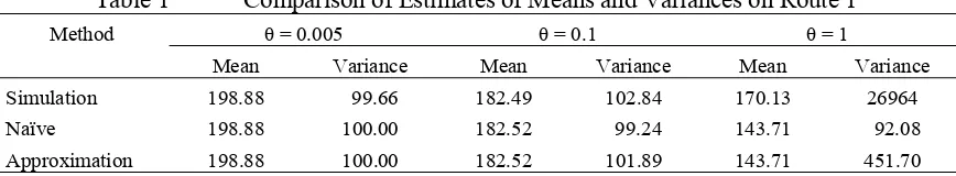
[image:17.612.90.524.293.373.2]

Table 1 compares the means and variances for Route 1 by the above three methods for various values of the logit choice parameter . In this two-link case, computing the mean and variance of flows on the other route is trivial, and so is not shown here.

Table 1 Comparison of Estimates of Means and Variances on Route 1

Method = 0.005 = 0.1 = 1

Mean Variance Mean Variance Mean Variance

Simulation 198.88 99.66 182.49 102.84 170.13 26964 Naïve 198.88 100.00 182.52 99.24 143.71 92.08 Approximation 198.88 100.00 182.52 101.89 143.71 451.70

When the logit choice parameter is relatively low ( =0.005), the random dispersion element in drivers’ travel costs is very high making them choose routes almost at random regardless of the measured (mean) cost, thus approximately equal numbers of drivers are expected to select each route, and our variation is approximately binomial. In this case as would be expected, the naïve approximation is sufficient to explain the variance in traffic flows. As expected, the approximation method adds little to the conditional covariance matrix in this case. It is noted also that the mean flows by all the three methods are identical to two digits.

In case of =0.1, the mean flows by all the three methods are again very close. However, the naïve variance underestimates the benchmark (simulation) variance. This underestimation of the variance is expected because the naïve method assumes fixed multinomial choice probabilities as opposed to the real case of day-to-day varying choice probabilities, i.e. it neglects one source of variability. Our approximation successfully corrects this underestimation by inflating the variance towards the benchmark simulation variance. While the magnitude of the correction required is not large, we cannot attach any significance to this as this is intended purely as an artificial, illustrative example.

(18)

solutions), resulting in a bimodal distribution. Thus, the variance is measuring some kind of system instability (in the same sense that one could calculate a variance for a deterministic periodic system) rather than random variation of a stationary variable. The naïve variance is not expected to explain such behaviour and hence is too small. Indeed, neither is the approximation method designed to explain such variation, and the corrected variance is seen to be far lower than the simulation variance. This is not surprising as we are estimating the variance of a bimodal distribution with an approximate Normal distribution, which is clearly not an ideal choice; nevertheless, it is partially successful in correcting the variance in the appropriate direction.

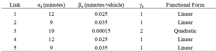
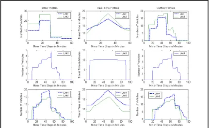
[image:18.612.114.469.356.492.2]

Example 2: This numerical example illustrates an application of the theory formulated in the earlier section to the case of a network with multi-link routes. Consider a five link network with links numbered as shown in Figure 1. It is worth noting that links 2 and 4 are shared by two paths hence require the flows to diverge and merge in space and time which is a common requirement in dynamic traffic assignment over networks serving multiple O-D pairs. Thus, even though this example deals with a single O-D pair, the principles described here can easily be extended to networks serving multiple O-D pairs.

Figure 1: Test Network Topology

On each of the five links whole-link type dynamic travel time functions of the general form )

t ( x )

t

( a

a a a a

γ

β + α =

τ are defined with parameter values as shown in Table 2.

Table 2 Network Parameters

Link a (minutes) a (minutes/vehicle) a Functional Form

1 12 0.025 1 Linear

2 9 0.035 1 Linear

3 10 0.00015 2 Quadratic

4 12 0.025 1 Linear

5 9 0.035 1 Linear

We note here that FIFO compliance is one of the important features of any dynamic traffic assignment model, as well as being an assumption of our approximation method, and so we confirm that FIFO has been monitored closely during the execution of the program and has

Destination Origin

Node 1 Node 2

3

2

1 4

[image:18.612.130.487.578.664.2]

(19)

been found satisfactory. On the demand side, we have modelled the demand spread over

4

L= departure periods each of κ=15 minutes duration with a varying profile thus indicated by, qk = [400 700 100 100].

For the dynamic network loading purposes, we assumed a minor time step of = 1 minute. In addition, we also retained a memory length of m=5 days with a memory weighting of

=

[image:19.612.92.523.295.560.2]

λ 0.5. The route choice is assumed to be based on a logit principle, and dynamic Stochastic User Equilibrium (SUE) flows are solved for using the Method of Successive Averages together with the dynamic network loading method as before. Figure 2 indicates the SUE profiles of inflow, travel time and outflow from various links on the network. We compare here the variance of the route flows by a similar set of alternative methods, viz., simulation, naïve and the method of approximation run to similar specifications as indicated previously.

Figure 2: Dynamic Network Loading Results (θ=0.1)

(20)

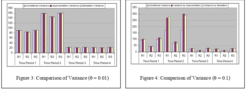
approximation method adds a correction term and lifts the flow variances close to the simulation variance.

CONCLUSIONS

In the present paper we have successfully made a first step at linking together the fields of network equilibrium theory, whole-link dynamic travel time models, and stochastic process models of the within- and between-day evolution of traffic flows over a network. In making this link, we have devised a computational procedure for estimating the equilibrium distribution of such a doubly dynamic stochastic process model, utilising information from a conventional stochastic user equilibrium model. A key element of the approximation is the computation of the Jacobian of the whole-link travel time mapping, which may have many applications beyond that discussed here. This research opens up many avenues for further research, including analysis of the stability of the dynamical process, application of the method to alternative forms of whole-link travel time model, and travel behaviour research investigating the impact of the various learning and decision parameters on the network flows.

ACKNOWLEDGEMENTS

The first author sincerely thanks UniversitiesUK and the University of Leeds for funding his research studies in England and ITS Leeds for the studentship being provided. The authors jointly thank Ronghui Liu for commenting on an earlier draft, and Malachy Carey, Richard Connors, Agachai Sumalee and Martin Hazelton for several thought provoking discussions and suggestions on this research. The authors also thank the anonymous referees for their useful comments and helpful suggestions.

0 20 40 60 80 100 120 140 160 180

R1 R2 R3 R1 R2 R3 R1 R2 R3 R1 R2 R3 Time Period 1 Time Period 2 Time Period 3 Time Period 4

Conditional Variance Approximation Variance Simulation Variance

0 50 100 150 200 250 300 350

R1 R2 R3 R1 R2 R3 R1 R2 R3 R1 R2 R3 Tim e Period 1 Time Period 2 Time Period 3 Tim e Period 4

[image:20.612.107.510.144.291.2]

Conditional Variance Variance by Approximation Variance by Simulation

(21)

REFERENCES

Astarita, V. (1996) A continuous time link model for dynamic network loading based on travel time function, J.B.Lesort ed. Proc. of 13th International Symposium on Transportation and Traffic Theory Elsevier, Oxford, U.K.,79-102.

Ben-Akiva, M., De Palma, A. and Kaysi, I. (1991) Dynamic network models and driver information systems, Transportation Research A 25(5), 251-266.

Cascetta, E. (1989) A stochastic process approach to the analysis of temporal dynamics in transportation networks, Transportation Research B, 23(1), 1-17.

Cantarella, G.E. and Cascetta, E. (1995) Dynamic Processes and Equilibrium in Transportation Networks: Towards a Unifying Theory, Transportation Science 29(4), 305-329.

Davis, G.A. and Nihan, N.L. (1993) Large Population Approximations of a General Stochastic Traffic Assignment Model, Operations Research 41(1), 169-178.

Friesz, T.L., Bernstein, D., Smith, T.E., Tobin, R.L. and Wie, B.W. (1993) A Variational Inequality Formulation of the Dynamic Network User Equilibrium Problem, Operations Research 41(1), 179-191.

Hazelton, M. and Watling, D. (2004) Computation of Equilibrium Distributions of Markov Traffic Assignment Models, Transportation Science 38(3), 331-342.

Horowitz, J.L. (1984) The stability of stochastic equilibrium in a two-link transportation network, Transportation Research B 18(1), 13-28.

Iida, Y., Akiyama, T., and Uchida, T. (1992) Experimental analysis of dynamic route choice behaviour Transportation Research B 26(1), 17-32.

Jha, M., Madanat, S. and Peeta, S. (1998) Perception updating and day-to-day travel choice dynamics in traffic networks with information provision, Transportation Research C 6(3), 189-212.

Nakayama, S., Kitamura, R., and Fujii, S. (1999) Driver’s learning and network behaviour: dynamic analysis of the driver-network system as a complex system, Transportation Research Record 1676, 30-36.

Watling, D.P. (1996). Asymmetric problems and stochastic process models of traffic assignment, Transportation Research B 30(5), 339-357.

Watling, D.P. (2002). A Second Order Stochastic Network Equilibrium Model. II: Solution Method and Numerical Experiments, Transportation Science 36(2), 167-183.