Chain Plot: A Tool for Exploiting Bivariate Temporal Structures

This is a repository copy of Chain Plot: A Tool for Exploiting Bivariate Temporal Structures. White Rose Research Online URL for this paper:

http://eprints.whiterose.ac.uk/74711/

Article:

Taylor, CC and Zempeni, A (2004) Chain Plot: A Tool for Exploiting Bivariate Temporal Structures. Computational Statistics and Data Analysis, 46 (1). 141 - 153 . ISSN 0167-9473

https://doi.org/10.1016/S0167-9473(03)00120-8

Reuse See Attached Takedown

If you consider content in White Rose Research Online to be in breach of UK law, please notify us by

Chain Plot: A Tool for Exploiting Bivariate Temporal

Structures

C.C. Taylor

Dept. of Statistics, University of Leeds, Leeds LS2 9JT, UK

A. Zempl´eni

Dept. of Probability Theory & Statistics, E¨otv¨os Lor´and University,

P´azm´any s´et´any 1/C, Budapest, H-1117

Abstract

In this paper we present a graphical tool useful for visualizing the cyclic behaviour of bivariate time series. We investigate its proper-ties and link it to the asymmetry of the two variables concerned. We also suggest adding approximate confidence bounds to the points on the plot and investigate the effect of lagging to the chain plot. We conclude our paper by some standard Fourier analysis, relating and comparing this to the chain plot.

1 Introduction

The idea we investigate in this paper has emerged during a relatively simple-looking problem in data analysis. We were given a data set from an automatic measurement station located at Szeged, Southeast-ern Hungary. Environmental (climate and pollution) measurements were collected with readings every half an hour over a 4-year period. For a detailed description and alternative analysis of the data set see Makra et al. (2001). The method we describe in this paper was found to be very useful for the data given. It is generally applicable to the analysis of bivariate time series with cyclic, or seasonal, components.

We suggest the following plot as a visualization of the joint behaviour of the daily pattern of certain pollutants. Let us suppose the time se-ries (Xt)Tt=1 and (Yt)Tt=1 have a periodic component with length N

(in our case Xt and Yt are half-hourly readings for two pollutants at

the time point t, so N = 48). Let

Xk = N

T

T /N

X

i=1

Xk+(i−1)N Yk = N

T

T /N

X

i=1

Yk+(i−1)N k = 1, . . . , N.

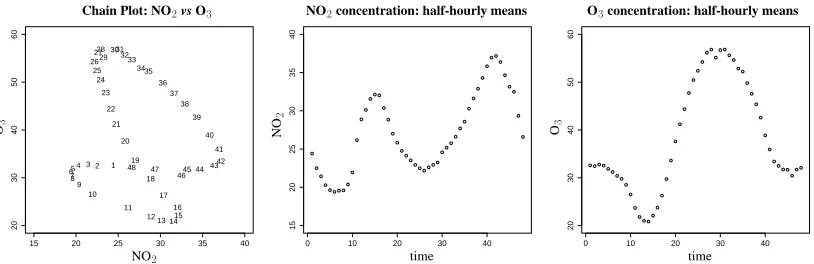
(1) Figure 1 is a scatter plot of these values on the x, y axis, labelled by k, together with the usual separate time series plot of the two components. In this example one of the series has a bimodal structure, whereas the other series is roughly unimodal though asymmetric. The chain-like pattern gave us some ideas for further investigation which we present in the following sections.

15 20 25 30 35 40

20 30 40 50 60 1 2 3 4 5 6₇ 8 9 10 11 12 13 1415

16 17 18 19 20 21 22 23 24 25 26 2728 29 3031 32 33 3435 36 37 38 39 40 41 42 43 44 45 46 47 48 NO2 O3

Chain Plot: NO2vs O3

0 10 20 30 40

15 20 25 30 35 40 time N O2

NO2concentration: half-hourly means

0 10 20 30 40

20 30 40 50 60 time O3

O3concentration: half-hourly means

We investigate behaviour of the chain plot for deterministic functions in Section 2, and bootstrap methodology for inference in Section 3. Some statistical applications are in section 4, and a brief discussion concludes the paper.

2 Chain plot for deterministic functions

In this section we consider continuous, deterministic functions rather than random variables, as this allows us to prove simple results, which have obvious applications to the original setup as well. We suppose our functions x(t) and y(t) to be bounded, continuous and defined for t ∈ [0,1]. We note here that the time-scale transformations have no effect on the suggested chain plot. Let us consider the simpler of the two, say x, as the reference function. As we want to get chain plots rather than open-ended line plots, we confine ourselves to the cases x(0) = x(1), y(0) = y(1) (which automatically holds for the motivating example of periodic time series). In this setup, the formal definition of the chain plot is A := {(x(t), y(t)) : t ∈ [0,1]}. This is of course a closed curve, and we shall investigate its properties below, which are relevant to the statistical problem under consideration.

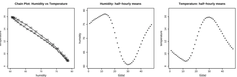
As a motivation of our results, we show another example of a chain plot in Figure 2 where we observe an almost one-dimensional be-haviour. This is substantially different from Figure 1. What is the main reason behind these differences?

60 65 70 75 80

8

10

12

14

16

Chain Plot: Humidity vs Temperature

humidity

temperature

1 23

45 67

891011141213 15 16 17 18 19 20 21 22 23 24 25 26 27 28 29 30 3132₃₃

34 35

36 37

38 39

40 41

42 43

44 45

46 47₄₈

0 10 20 30 40

60

65

70

75

80

Humidity: half−hourly means

humidity

time

0 10 20 30 40

8

10

12

14

16

Temperature: half−hourly means

temperature

time

Fig. 2. Half-hourly means for climate variables: connected chain plot and marginal plots

we might omit the arguments if it does not cause confusion.

2.1 The simplest case

In this section we introduce the main notions of this paper in a setup which allows an easy interpretation.

Definition 1 We say our reference function x is simple if it is strictly monotonically increasing in [0, t0] and strictly monotonically

de-creasing in [t0,1].

Remark 1 We note that we have not claimed the derivative of x to exist at all the points.

We supposed that x(0) = min{x(t) : t ∈ [0,1]}, but it is not a real condition, as the endpoints of the interval can be chosen arbitrarily. We have not posed any conditions for the set {x(t) : t ∈ [0,1]}, but in order to make the chain plot area for different pairs of functions

(x, y) to be comparable, it is advised to normalize all the variables.

There are lots of real-life cases, where one of the components of the bivariate time series can be considered as a simple function (temper-ature over a day being the most obvious example, see also Figure 2). The conditions of the following lemma are not at all unrealistic in real-life examples.

Let x be a simple function and define x1 : [0, t0] → R as x|[0,t0] and x2 : [t0,1] → R as x|[t0,1].

Lemma 1 Let x be simple and suppose that A consists of a single chain (i.e. it is homeomorphic to a circle). Then

A =

Z x(t0)

x(0) y(x

−1

1 (u))du−

Z x(t0)

x(0) y(x

−1

2 (u))du

. (2)

along the x-axis:

{(x(t), y(t)) : t ∈ [0,1]}= {(u, y(x₁−1(u))) : u ∈ [x(0), x(t0)]} ∪ {(u, y(x−₂1(u))) : u ∈ [x(0), x(t0)](3)}

As the two parts defined in (3) have no intersection points in their interior, the assertion (2) is a simple consequence of (3).

In the remainder of this section we use a transformation, which is again the easiest to be introduced for simple reference functions. It is similar to the probability-integral transformation — see Embrechts et al. (1999) for example — used to transform marginal distributions of bivariate random variables to uniform ones. We use the transforma-tion for one coordinate only, in order not to change the value of A. In our actual deterministic world, the role of the uniform distribution is of course played by the function x(t) = ct or x(t) = c(1−t). Let

(˜x(t),y(t)) :=˜

    

   

(2tx(t0), y(x−11(2tx(t0)))) if0 ≤t ≤ 0.5

(2(1−t)x(t0), y(x−21(2(1−t)x(t0)))) if0.5< t ≤ 1

(4)

Remark 2 It is obvious that transformation (4) does not affect the chain plot. x˜ is a simple function, too.

We now reformulate — and at the same time generalize — our previ-ous result (Lemma 1). This makes it easier to understand the meaning of the area A we investigate and even more importantly it allows fur-ther generalizations.

Proposition 1 Let x be simple. Then

A = Z 0.5

0 |y(u)˜ −y(1˜ −u)|du. (5)

Proof By Remark 2 we know that A can be calculated using the functions (˜x,y)˜ . Sincex is simple A is a union of the areas of simple chains, defined by the intersection points: {u∈ [0,1] : ˜y(u) = ˜y(1−

1. It only has to be observed that the continuity of x and y implies that on the whole domain of integration either y(u)˜ > y(1˜ −u) or

˜

y(u) < y(1˜ −u), so we can move the absolute value into the integral.

Formula (5) turns out to be important for calculating the area of a chain plot for observed data.

Definition 2 The asymmetry index of y with respect to a simple x is defined as AI(y, x) := A.

Analogues of this definition can be found in the literature: for the dependence function of bivariate extremes, an analogous definition was given in Villa-Diharce (2001). Our definition is easily motivated, see the first of the following properties:

(i) AI(y, x) = 0 ⇐⇒ y(u) = ˜˜ y(1 −u) holds for all u ∈ [0,1]. This means that the behaviour of y during the period of which

x increases is exactly symmetric to its behaviour during the de-crease of x.

(ii) If 0 ≤ y ≤ 1, then 0 ≤ AI(y, x) < 1, where the latter in-equality can be changed into “smaller or equal” if we allow for noncontinuous y: y = δ[t0,1] has AI(y, x) = 1.

(iii) The visible asymmetry in Definition 2 can be easily resolved if

y is itself simple, since then we can choose y as the reference function and thus we are allowed to define AI(x, y) = A as well.

Neither co-ordinates of Figure 1 are simple functions (even after shifting the time scale to ensure x(0) = min{x(t)}), so we must introduce necessary modifications in order to cover this and similar cases.

2.2 Some generalizations

So we loosen the conditions imposed for our reference function x to such an extent only, which allows the investigations of practically all real-life applications.

Definition 3 We say our reference function x is normal if there are points 0 = s1 < t1 < s2 < t2 < s3 < · · · < tm < sm+1 = 1

such that x is strictly monotonically increasing over [si, ti] and x

is strictly monotonically decreasing over [ti, si+1] or it is constant

over the whole interval [si, si+1] (i = 1, . . . , m) and min{x(t) : t ∈

[0,1]}= x(0).

Remark 3 The simple reference functions are exactly those normal ones, which are non-constant and for which m = 1.

Now the definition of the area of the chain plot is far from straight-forward, as in this more complicated case several inner loops and un-usual configurations might arise (we do not think them to be very common in real applications). We choose one possible definition, which is just an iteration of cases defined in the previous section.

Let A be a chain plot which intersects itself by finitely many points. Then we define its area recursively as A = A1 + A∗, where A1 is

the area of the first subchain (which is obtained simply by drawing the plot until it is first closed). We then omit this part from the chain (A∗ is the remainder), and define its area similarly (this is denoted by

A∗). More formally:

Step 1 Let u1 := min{u : ∃v < u : x(u) = x(v), y(u) = y(v)}

(let v1 be the corresponding v) and the chain A1 := {(x(t), y(t)) :

v1 ≤ t ≤ u1}. (It should be noted that extreme cases, where one

segment of the chain exactly coincides with another segment, are excluded from this definition — but one can get rid of such parts by moving one of its components slightly, for example).

Step 2 The remaining part of the chain is then {(x(t), y(t)) : 0 ≤

t ≤ v1} ∪ {(x(t), y(t)) : u1 ≤ t ≤ 1} and go back to Step 1 (to

find the next sub-chain etc.)

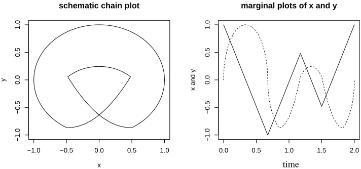
certain area twice (see Figure 3), but it seems to be logical, as these parts play a multiple role in the asymmetry.

−1.0 −0.5 0.0 0.5 1.0

−1.0

−0.5

0.0

0.5

1.0

schematic chain plot

x

y

0.0 0.5 1.0 1.5 2.0

−1.0

−0.5

0.0

0.5

1.0

marginal plots of x and y

x and y

time

Fig. 3. Left: A schematic chain plot, in which there is a region which is counted twice when the total area is calculated. Right: the two functions x(t) (line) andy(t) (dashed).

Now we have reduced our task of calculating the area of a chain plot, to the calculation of Ai, which is homeomorphic to a circle — but of

course not always simple in the sense of our Definition 1. Practical calculations of such an area can easily be performed by numerical methods. But in order to prepare the statistical procedures of section 3 we sketch an iterative algorithm for the reduction of the normal case to the sum of simple ones as follows.

For a non-intersecting chain plot with a normal reference function, we can calculate its area iteratively: Let us use the notation of definition 3 and let ε > 0 be so small that ∃ u0 ∈ [0, t1] : x(u0) = x(s2)−ε.

Then the line segment

I := {(x(s2)−tε, y(s2)−(y(s2)−y(u0))t) : t ∈ [0,1]

is entirely within the closed curve. Now the chain

{(x(u), y(u)) :u0 ≤ u ≤ s2} ∪I (6)

is a chain with a simple reference function and the x coordinate of the remainder chain

has exactly one less maximum point, so the iteration is finished in just a finite number of steps.

As a final remark, we mention that the total area of the chain plot is the sum of local asymmetries for subchains, corresponding to the constructed simple parts of the normal reference function.

3 Statistical applications

3.1 Asymmetry index-calculation for observed data

Using the notions introduced in the previous section, one can calcu-late the asymmetry index for the observed data. In order to do so, one only needs to interpolate the values between the observation points

(Xt, Yt) and (Xt+1, Yt+1). The simplest method is the linear

inter-polation, which we preferred in the current paper.

Carrying this out for the data under investigation, we got the follow-ing results. After normalizfollow-ing both variables so that the minimum is 0 and the maximum is 1 — which is preferred here to the more usual normalization based on the standard deviation, since that would allow arbitrarily large values for A in spite of the bounded variance — we get area 0.453 for the chain plot in Figure 1 (NO₂ vs. O₃) and 0.053

for the chain plot in Figure 2 (humidity vs. temperature). For a chain plot which forms a circle, the (normalized) area is π/4 = 0.785, and a square gives area 1 which is the maximal value for plots which only include areas once. For the plot in Figure 3 the asymmetry index is

0.879.

3.2 Alignment and Lagging

the first part of the series is “aligned” (though possibly with opposite sign) when the y variable is lagged +2 whilst the second part of the day is closely aligned when the y variable is lagged −4. This means that by finding those lags which provide the smallest area of the chain plot, we can find those shifts where the two variables show the most symmetrical behaviour (this lag can be interpreted as the lag for the effect of one variable on another).

20 25 30 35 40

20 30 40 50 60 1 2 3 4 5 67_{8 9}

10 11

12 13141516

17 18 19 20 21 22 23 24 25 26 27 2829

3031323334 3536 37 38 39 40 41 42 43 44 45 46 47 48 NO2 O 3

O3lagged 1

20 25 30 35 40

20 30 40 50 60 1 2 3 4 5 6789 10

11 12

13 141516 17 18 19 20 21 22 23 24 25 26 27 28 29 30

3132333435 36 37 38 39 40 41 42 43 44 45 46 47 48 NO2 O 3

O3lagged 2

20 25 30 35 40

20 30 40 50 60 1 2 3 4 5 67 8 910 11

12 13 14 15 16 17 18 19 20 21 22 23 24 25 26 27 28 29 3031

3233 343536 37 38 39 40 41 42 43 44 45 46 47 48 NO2 O 3

O3lagged 3

20 25 30 35 40

20 30 40 50 60 1 2 3 4 5

678 910 11 12 13 14 15 16 17 18 19 20 21 22 23 24 25 26 27 28 29 30 3132 3334353637

38 39 40 41 42 43 44 45 46 47 48 NO2 O 3

O3lagged 4

20 25 30 35 40

20 30 40 50 60 1 2 3 4 5 6 78 9 10 11

12 13 1415 16 17 18 19 20 21 22 23 24 25 26 2728

2930 3132 33 34 35 36 37 38 39 40 41 4243 44 45 46 47 48 NO2 O 3

O3lagged –1

20 25 30 35 40

20 30 40 50 60 1 2 3 4 5 6 7 8 9 10 11

12 13 1415 16 17 18 19 20 21 22 23 24 25 26 27 28 29303132

33 3435 36 37 38 39 40 41

42454344 46 47 48 NO2 O 3

O3lagged –2

20 25 30 35 40

20 30 40 50 60 1 2 3 4 5 6 7 8 9 10 11

1213 14 15 16 17 18 19 20 21 22 23 24 25 26 27 28 29303132

33 3435 36 37 38 39 40 41

42434445 46 47 48 NO2 O 3

O3lagged –3

20 25 30 35 40

20 30 40 50 60 1 2 3 4 5 6 7 8 9 10 11 1213 14 15

16 17 18 19 20 21 22 23 24 25 26 27 28 29 3031 32 33 3435 36 37 38 39 40 41

424344 45 46 47 48 NO2 O 3

O3lagged –4

Fig. 4. Connected chain plots for lagged series. Top row: positive lags; Bottom row: nega-tive lags

3.3 A method for testing symmetry

Our aim in this subsection is to give a procedure for testing symmetry between the variables. It is worth mentioning that in some cases, the physical processes behind the observed data suggest time lags (see Figure 4). In order to cope with this phenomenon, we first minimize the asymmetry index with respect of possible lags:

Amin := min_m AI(Xt, Yt−m) (8)

From now on let us suppose that the Y has been shifted so that the question is the symmetry of (Xt, Yt) is the most symmetric data set

for which the symmetrical behaviour with respect to the reference X

symmetry be accepted, based on an observed asymmetry index A?

In order to tackle this question, we might either use parametric mod-elling with a symmetric model:

Yt = Xt +εt (9)

where in the simplest case εt can be considered as an i.i.d. sequence

of 0-mean random variables. For such models more or less straight-forward methods for statistical inference are available. An obvious disadvantage of such an approach is that the cause of the possible rejection is not clear: it might well happen that there is just an ac-ceptable level of discrepancy from symmetry, and rejection is only based on the poor fit of the model. We thus suggest an alternative nonparametric method, focusing only on the symmetry.

Let us first suppose that the reference function constructed by inter-polation is simple. If it is only normal, then the procedure of (6–7) can be used to cut the curve into simple parts and then the symmetry of these parts can be tested independently. Let us use the transforma-tion ∼ defined in the previous section in (4). This is of course based on the observed averages X and Y , but from now on we omit the overline, when using ∼.

Our method relies on the fact that the area for the normalized AI can be approximated by

1 n

n/2−1

X

k=1

|Y˜(k/n)−Y˜(1−k/n)| (10)

(see (5), we supposed n to be an even number). Equation (10) shows that it is much more useful to base our procedures on the estimated values Y˜((k/n)) rather than the observed Y˜t, for which the

contribu-tion very much depends on the difference X˜t+1−X˜t. Let us introduce

the notation D(k/n) := ˜Y((k/n))−Y˜((1−k/n)) and consider the increments of the process D(k/n): δk := D(k/n)−D((k−1)/n) for

k = 1,2, . . . , n/2. It is obvious that Pn/2

k=1δk = D(1/2)−D(0) = 0

and that part of Equation (10) where there is no sign change (i.e. the absolute value is not needed) can be expressed as Pn/2

so we get the maximal value if the δ values are ordered.

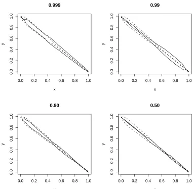
Now we can describe the procedure we suggest: if we generate a random permutation of the set {1, . . . , n/2} and permute the vector

(δ1, . . . , δn/2) then we get another closed curve. If there was no

asym-metry between the variables, then we could suppose that the original permutation was just a typical one, so the area of the original curve would be near to this generated one.

If we repeat the permutation procedure M times and calculate (10) for all, then we get M different possible values of the symmetry in-dex. If the observed AI is larger than the 95 (99 etc)% quantile of this observed distribution, then the symmetry can be rejected.

There is an open question how to choose n in Equation (10). We sug-gest to use the same number of points as for the original observations. This could be investigated, but for an X with constant derivative we use just the original observations. Another point against a too refined grid is the extensive computing time and that in such cases almost al-ways there is strong dependence among neighbouring values, which indicates that there is little gain in using all of them.

The suggested approach shows similarities to the methods presented in Schmid and Trede (1995), where the classical two sample prob-lem is tested by a method, based on the area between two curves. The asymptotic distribution of their test statistic is the integral of the Brownian bridge (see Shepp, 1982 for its tabulated distribution). We also get this limit distribution for the scaled and randomized sequence if certain mixing conditions can be supposed for the sequence δ, but as in our problems we have a definite, not too large number as n, we do not exploit this idea here.

plots have a very similar structure, and the asymmetry index itself was small. However, this sample size of n = 1460 means that the chain plot is very smooth and so there is little variability in the resulting δk.

0.0 0.2 0.4 0.6 0.8 1.0

0.0

0.2

0.4

0.6

0.8

1.0

0.999

x

y

0.0 0.2 0.4 0.6 0.8 1.0

0.0

0.2

0.4

0.6

0.8

1.0

0.99

x

y

0.0 0.2 0.4 0.6 0.8 1.0

0.0

0.2

0.4

0.6

0.8

1.0

0.90

x

y

0.0 0.2 0.4 0.6 0.8 1.0

0.0

0.2

0.4

0.6

0.8

1.0

0.50

x

y

4 Extensions

4.1 Correlations

The cross-covariance between (Xt)Tt=1 and (Yt)Tt=1 at lag j is

esti-mated by

cxy(j) =

1 T

T−j

X

t=1

(Xt −X)(Yt+j −Y) j = . . . ,−1,0,1, . . .

and the cross-correlation at lag j is estimated by

rxy(j) =

cxy

sxsy

where s2_x = T−1P

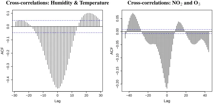
(Xt − X)2. For the type of data considered here

most of the cross-correlation can be attributed to the fact that both Xt

and Yt have very pronounced periodic components. For example, for

the data considered in Figures 1 and 2 the cross-correlations are given in Figure 6. In such cases, we ought to consider the correlation after

−30 −20 −10 0 10 20 30

−0.4

−0.3

−0.2

−0.1

0.0

0.1

Lag

ACF

Cross-correlations: Humidity & Temperature

−40 −20 0 20 40

−0.20

−0.15

−0.10

−0.05

0.00

0.05

Lag

ACF

Cross-correlations: NO2and O3

Fig. 6. Cross-correlations of bivariate data

allowing for the periodic effects. This can be done by considering the cross-covariance at lag j for points at seasonal time k, which is given by

cxy(k, j) = N

T

T /N−k

X

t=1

for k = 1, . . . , N, j = . . . ,−1,0,1, . . . , N −j where Xk and Yk+j

are given in Equation (1). The adjusted sample cross-correlation can be estimated in an analogous manner. Incorporating all of this infor-mation on the chain plot is difficult, since we now have N cross-correlation plots to display. However, if we initially consider j = 0

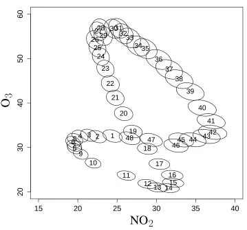
and use a normal approximation to describe the joint distribution of

Xk and Yk, then we can include 100(1 − α)% confidence limits

around each point in the chain plot. An example is shown in Figure 7 which shows how the variability in the two variables changes over time. An efficient way to construct such contours is to use polar co-ordinates as follows.

Let θ be a sequence of length l angles in [0,2π], and form the l×2

matrix M = [cosθ,sinθ]. Given k, j form the covariance matrix for the relevant data, say

Σ =



   

cxx(k, j) cxy(k, j)

cyx(k, j) cyy(k, j)



   

Now solve v = Σ−1MT and then plot polar co-ordinates r(θ), θ

around (Xk, Yk) where r(θ) is a vector of length l determined by

r2(θ) = χ

2

2(1−α)

vT_Mu

where u = (1,1)T and χ₂2(1−α) is the 100(1−α)% point from a

χ2 distribution with 2 degrees of freedom.

15 20 25 30 35 40

20

30

40

50

60

Chain Plot with 90% Confidence Interval

1 2 3 4 5 6₇ 8

9 10

11 12

13 1415 16 17 18 19 20 21 22 23 24 25 26

2728 29

3031 32

33 3435

36 37

38

39

40

41

42 43 44 45 46 47

48

NO

O

3

Fig. 7. Modified chain plot with 90% confidence intervals (using a multivariate normal approximation) based on the conditional covariance at each time point

4.2 Fourier Analysis

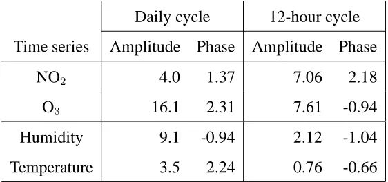
A straightforward Fourier analysis was made harder by the large number of missing values. So, in order to compare with the above results we fitted a linear model corresponding to only daily and 12 hourly periods (Bloomfield, 2000). That is, for each time series, we fitted the model:

Xt = α+ R1cos(ω1t+ φ1) +R2cos(ω2t+φ2) +εt

where Ri, φi, i = 1,2 are the fitted amplitudes and phases,

respec-tively, corresponding to the frequencies ωi, with ωi corresponding to

in Table 1.

Daily cycle 12-hour cycle

Time series Amplitude Phase Amplitude Phase

NO2 4.0 1.37 7.06 2.18

O3 16.1 2.31 7.61 -0.94

Humidity 9.1 -0.94 2.12 -1.04

Temperature 3.5 2.24 0.76 -0.66

Table 1

Amplitude and phases corresponding to two fitted periods for each of four time series

For the climate time series (humidity and temperature) the dominat-ing period is the daily cycle, and the two phases are very similar. This implies that the asymmetry index A is small (see Figure 2) and vi-sually we would expect the chain plot to be long and thin. For the two pollutants, the phases for the daily cycle are very different, and the 12-hourly cycle is relatively more important for NO₂ than for O₃. These values are consistent with the chain plot analysis (due to the phase differences, the lagging was necessary for achieving some symmetry), but we think not so immediately informative. In particu-lar, it is not obvious how the two series can be partially aligned using the given phases for the two cycles.

5 Discussion

We end our paper with some comments on the use of the suggested graphical tool. As here we have practically three dimensions to in-vestigate (time+two variables), the traditional sequence of bivariate scatterplots (2 time series plots plus a scatterplot in our case) do not give a clear picture of the evolution of the relation over time.

Acknowledgements: We acknowledge support from the British Council and the Hungarian Ministry of Education under the British-Hungarian Academic Research Programme.

References

Bloomfield, P. 2000. Fourier Analysis of Time Series: An Introduction (second edition). John Wiley, New York.

Embrechts, P., McNeil, A. and Straumann, D. 1999. Correlation and dependency in risk management: properties and pitfalls. Preprint ETH, Z¨urich. www.math.ethz.ch/∼embrechts.

Makra, L., Horv´ath, Sz., Taylor, C.C., Zempl´eni, A., Motika, G. and S¨umeghy, Z. 2001. Modelling air pollution in countryside and urban environment, Hungary. Proc. of the 2nd International Symposium on Air Quality Management at Urban, Regional and Global Scales. Is-tanbul, Turkey. pp. 189-196. Eds.: Topcu, S. Yardim, M.F. and Ince-cik, S.

Schmid, F. and Trede, M. 1995. A distribution free teset for the two sample problem for general alternatives. Comput. Stat., Data Anal. 20, p. 409-419.

Shepp, L.A. 1982. On the integral of the absolute value of the pinned Wiener process - calculation of its probability density by numerical integration. Ann. Probab. 10, p. 240-243.