This is a repository copy of
Neuro-dynamic programming for cooperative inventory control
.
White Rose Research Online URL for this paper:
http://eprints.whiterose.ac.uk/89779/
Version: Accepted Version
Proceedings Paper:
Bauso, D., Giarré, L. and Pesenti, R. (2004) Neuro-dynamic programming for cooperative
inventory control. In: Proceedings of the American Control Conference. Proceeding of the
2004 American Control Conference , June 30 -July 2,2004 , Boston, MA, USA. IEEE ,
5527 - 5532. ISBN 0780383354
[email protected] https://eprints.whiterose.ac.uk/ Reuse
Unless indicated otherwise, fulltext items are protected by copyright with all rights reserved. The copyright exception in section 29 of the Copyright, Designs and Patents Act 1988 allows the making of a single copy solely for the purpose of non-commercial research or private study within the limits of fair dealing. The publisher or other rights-holder may allow further reproduction and re-use of this version - refer to the White Rose Research Online record for this item. Where records identify the publisher as the copyright holder, users can verify any specific terms of use on the publisher’s website.
Takedown
If you consider content in White Rose Research Online to be in breach of UK law, please notify us by
Neuro-Dynamic Programming for Cooperative Inventory Control
Dario Bauso, Laura Giarr´e and Raffaele Pesenti
Abstract— In Multi-Retailer Inventory Control the possi-bility of sharing set up costs motivates communication and coordination among the retailers. We solve the problem of find-ing suboptimal distributed reorderfind-ing policies which minimize set up, ordering, storage and shortage costs, incurred by the retailers over a finite horizon. Neuro-Dynamic Programming (NDP) reduces the computational complexity of the solution algorithm from exponential to polynomial on the number of retailers.
I. INTRODUCTION
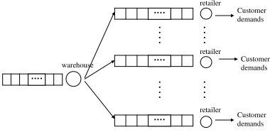
We consider a two echelon, one-warehouse multi-retailers inventory system. Each day, a stochastic demand mate-rializes at each node. Unfulfilled demand is backlogged. Retailers observe their own inventory level, communicate and make decisions whether to reorder or not from ware-house to fulfill the expected demand. Ordered quantities plus inventory at hand may not exceed storage capacity at each store. Reordering occurs by means of a single track which serves all the retailers. Set up costs are shared among all retailers who reorders, also called active retailers. This motivates a certain coordination of reordering policies. The system under concern is depicted in Fig. 1.
••••
••••
••••
•••• • • • •
• • • • warehouse
Customer
demands •
• • •
retailer
retailer retailer
Customer
demands
Customer
demands •
[image:2.612.72.262.431.524.2]• • •
Fig. 1. One-warehouse multi-retailer inventory system
Decentralization of policies under partial information is the main focus in [6]. In [10] the authors analyze the benefits of the information sharing on the performance of the entire chain. In [1] issues are discussed, regarding the use of different kinds of penalties, transfer prices and cost sharing schemes to improve the coordination of policies optimized on a local basis.
In a static context, i.e., for fixed day and fixed inventory levels, we introduced in [3], a distributed consensus protocol
D. Bauso is with DINFO, Universit`a di Palermo, 90128 Palermo, Italy
L. Giarr´e is with DIAS, Universit`a di Palermo, 90128 Palermo, Italy
R. Pesenti is with DINFO, Universit`a di Palermo, 90128 Palermo, Italy
[7] for estimating the number of active retailers and coor-dinating the reordering policies. Each retailer is assumed to choose a fixedthreshold policy, with thresholdli on the
number of active retailers. In other words one defines its
intention to reorder only if at least other li −1 retailers
are willing to do the same. We proved that consensus on the number of active retailers is asymptotically globally reached and coordination is the same that if the decision making process would be centralized, namely, any retailer has access to the thresholds of all other retailers and chooses whether to reorder or not. The proposed distributed protocol has the advantage that the retailers do not communicate their threshold policy to reach consensus on the number of active retailers.
This paper extends the aforementioned results to a dy-namic inventory control context, i.e., where inventory levels change each day. We show that the threshold policies assumed in [3], are strictly connected to the well known
(s, S) policies [9], [8]. In some cases, we prove that a
optimal policy, for each ith retailer, is to order only in
conjunction with at least other li−1 retailers. We prove
also that the threshold li can be computed locally by
the ith retailer depending on the current inventory level
and expected demand. This is possible by implementing a distributed Neuro-Dynamic Programming (NDP) algorithm polynomial on the number of retailers, which avoid the curse of dimensionality and reduces errors due to model uncertainties.
This paper is organized as follows. In Section II we de-velop a hybrid model for the cooperative inventory control
problem. In Section III we prove that the cost function isK
-convex and hence can be efficiently computed in a reduced number of points. We show also that threshold policies on the number of active retailers are optimal. In Section IV we presents the NDP algorithm. In Section V we provide conclusions.
II. HYBRIDMODEL
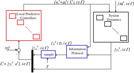
In this section we present a novel hybrid model for the multi-retailer inventory system (see, e.g., Fig. 2). In
particular, in Subsection II-A, we model the n decoupled
inventory subsystems. In Subsection II-B, we model the information flow among the subsystems. In Subsection II-C, we introduce the structure of the local controllers and formally state the problem.
A. System Dynamics
Consider a network G = (V,E); each retailer is a
node vi ∈ V, where i ∈ Γ := {1,2, ..., n}, and each
communication link is an edge e = (vi, vj) ∈ E; i, j =
Information Protocol
{Ii k
= [yi k
, a k
],i∈Γ}
{ui k
=µi k
( Ii k
),i∈Γ}
System Dynamics Local Predictive
Controllers
{yi k
,i∈Γ} {zi
k
(τ),i∈Γ}
sample
{zss k
,i∈Γ}
{ωi k
,i∈Γ}
ref
T +
[image:3.612.66.295.73.198.2]-
Fig. 2. Block Diagram of the closed loop inventory system.
of the setS. The model inputuk
i is the quantity of inventory
ordered by theith retailer at each stagek= 0,1, ..., N−1.
We model with ωk
i the stochastic demand faced by theith
retailer.
Theith inventory subsystem is a finite-state discrete-time
model, that for alli∈Γtakes on the form
xki+1=x k i +u
k i −ω
k i.
The inventory at hand plus inventory ordered may not exceed storage capacity as is expressed in the following equation
xki +u k
i ≤Cstore.
The ith outputyk
i, referred to as sensed information, is
yki =x k i,
i.e., each retailer observes only his inventory level.
B. Consensus Protocols
The information flow is managed through a distributed
protocol Π ={(fi, hi, φi) : for alli∈ V}
˙
zik(τ) = fi(zkj(τ), for allj∈Ni),0≤τ≤T,(1a)
zik(0) = hi(yik), (1b)
ak = φi(zssk) (1c)
where:
• fi:ℜn→ ℜdescribes the dynamics of the transmitted
information of theith node as a function of the
infor-mation both available at the node itself and transmitted by the other nodes, as expressed in (1a);
• hi : Z → ℜ generates a new transmitted information
vector given his output at the stage k, as described
in (1b);
• φi :ℜ → Z estimates, based on current information,
the aggregate info (1c).
Here Ni is the neighborhood of theith retailer,Ni={j∈
Γ : (vi, vj)∈ E} ∪ {i}, i.e., the set of all the retailersj that
are connected to iandiitself and
zkss= lim τ→T−
zi(kT+τ), for alli∈Γ, (2)
represents the steady state value assumed by zk
i(τ)within
the interval[kT,(k+ 1)T].
We refer the reader to [7] for studies on the convergence of consensus protocols. For given scenario, defined by the full state vector,xk ={xk
i, for alli∈Γ}, the converging
value of the transmitted information, ak
i, plus the sensed
information, yk
i constitute the partial information vector,
Iik= [y k i, a
k
i]available to theith retailer.
C. Local Predictive Controllers
The local controllers compute the following cost over a finite horizon
Ji( ˆIik, u k i) =E
gi( ˆI
N i ) +
NX−1
ˆ
k=k
(αkˆgi( ˆI
ˆ
k i, u
ˆ
k i))
(3)
whereIˆk
i is the predicted information andαkis the discount
factor at stagek. The stage costgi( ˆIik, uki, k)is defined as
gi( ˆIik, u k i, k) =
K akδ(u
k i) +cu
k
i +pE{max(0,−yˆ k+1
i )}
+hE{max(0,yˆki+1)}
,
(4)
whereK represents the set up cost, c is the purchase cost
per unit stock,pis the penalty on storage,hthe penalty on
shortage, and δ(ui(k)) is zero if the ith retailer does not
reorder, and one if he reorders.
As will be clear later on, the idea of the solution algorithm is to use a simulation-based tunable predictor of the form
ˆ
Iik+1=
ˆ
yik+1
ˆ
aki+1
=
xk i +u
k i −ωˆ
k i
ψi(aki, u k i)
(5)
In (4) we assume that the set up cost is equally shared among the active retailers.
We report hereafter the formalization of the problem under concern. Given a set of retailers reviewed as dynamic
agents of a network with topologyG= (V,E).
Problem (Local Controllers Synthesis) For each ith retailer, determine the reordering policy uk
i =µ(I k i), that
minimizes theN-stage individual payoff defined in (3). Subproblem(Protocols Design)Determine a distributed protocolΠwhich maximizes the set of active retailersAΠ.
III. DYNAMICPROGRAMMINGAPPROACH
In this section, we prove that the inventory must be or-dered in quantity thus to fulfill exactly the expected demand for the upcoming days, as summarized in Theorem 3.1. We provide an intuitive explanation of such a result.
LetKk= K
ak the set up cost charged to each retailer that reorders at stage k, and dk
i =xki +uki, the instantaneous
inventory position, i.e., the inventory level just after the order has been issued. Then we claim as follows.
• If the setup costKk decreases with time (in the future
more and more retailers are interested in reordering) retailers place short term orders. Optimal policies are multiperiod policies(sk, Sk), with a unique lower and
• On the contrary, if the setup costKk
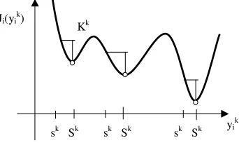
increases with time (in the future less and less retailers are interested in reordering), retailers place long-term orders. Op-timal policies are multiperiod policies (sk, Sk) with
multiple thresholds at different inventory levels (see, e.g., Fig. 4).
Kk
Sk
sk
Ji(yik)
yi
k
Fig. 3. Intuitive plot of the cost when the set up cost decreases with time: single thresholds(sk
, Sk
).
Kk
Sk
sk
Ji(yik)
yi
k
Sk
sk sk Sk
Fig. 4. Intuitive plot of the cost when the set up cost increases with time: multiple thresholds(sk
, Sk
).
A. Searching for Structure: K-convex analysis
To show that the individual objective functions, Ji; i∈
Γ, have at most N local minima, we, first, apply the DP
algorithm (6)-(7) to minimize the cost (3). The Bellman’s
equation is then rearranged by defining a new functionH(·)
as in which verifies theKi-convexity property, whereKiis
the maximum set up cost incurred by theith retailer over the
horizon. Exploiting the definition of the inventory position
di and of the set up costKk, we rewrite the stage cost (4)
as
gi(d k i, a
k
) = Kkδ(uki) +cu k
i +pE{max(0,−(d k i −ω
k i))} +hE{max(0, dk
i −ω k i))}.
By applying the dynamic programming algorithm, we have
JiN(I N
i ) = 0, (6)
Jk i(I
k
i) = min uk
i∈U
[gi(dki, a
k) +αk+1
E{Jik+1(Iik+1)}]. (7)
Let us define the new function
Gk
i(dki, ak+1) =cdki +E{pmax(0,−(dki −ωki))
+hmax(0, dk i −ω
k i) +J
k+1
i (I k+1
i )},
and rewrite the Bellman’s equation (7) as follows
Jk
i(Iik) =−cixki+ min dk
i≥x
k i
[Kk+Gk
i(dki, ak+1), Gki(xki, ak+1)].
(8)
Note that if we can show thatJik+1 is Kk
-convex then
Gk
i is also Kk-convex and the Bellman’s equation (8) has
a unique minimizer.
Indeed, it has been proved in [4] that Kk-convexity of
Gk
i(di, ak+1)impliesKk-convexity ofJik(Iik).
This represents a sufficient condition that guarantees optimality of multiperiod(sk
i, Ski)order-up-to policies.
We recall that sk
i represents the minimum threshold on
inventory level below which retailers reorders to restore levelSk
i.
Let us remind thatSk
i minimizesGki(·, ak+1)and
thresh-oldsk
i verifies
Gki(s k i, a
k+1) =
Gki(S k i, a
k+1) +
Kk.
Now, let us callsk
i, the threshold which corresponds to
the assumption that theith retailer is charged the whole set
up cost; namely we haveKk
i =K;i∈Γ. At the same way,
let us define withsithe threshold computed as if all retailers
would share equally the setup costs; thus, each retailer is
charged a set up costKk
i = K
n, namely onenth of the entire
costK. We now explicit dependence of thresholdsk
i on set
up cost Kk
i by defining the function ski( K
ak) for which it holdssk
i ≤ski(·)≤ski.
Now, let us call
Hik(d k i, a
k
) = min
yk
i≥x
k i
[Kk+Gki(d k i, a
k+1), Gk i(x
k i, a
k+1)].
In the following, we considerak a parameter and show
that the individual objective function,Jk
i(xi);i∈Γ, which
is generically non convex, has all local minima coincide with the demand summed over one or more days.
Theorem 3.1: Solutions of the Bellman’s equation (7) are
at most N −k different multi period policies (ski, S
k i),
where Sk
i ∈ {
PM
j=kω j
i;M = k, k + 1, ..., N} and
thresholdsk
i verifiesG
k i(s
k i, a
k+1) =Gk i(S
k i, a
k+1) +Kk
. Policy are associated to different intervals of inventory levels.
Proof: The essential idea is that the cost is piecewise linear. This is evident in the Bellman’s equation where the costJk
i is the summation of a piecewise linear stage costgki
(with unique global minimum atωk
i) and a piecewise linear
future cost (with potential local minima atωk
i +S k+1
i ).
An immediate consequence of the above theorem is that the set of feasible decisions is finite and each element represents the exact ordered quantity to fulfill the expected
demand for the upcoming1,2, ..., N days.
B. Threshold Reordering Policies
[image:4.612.66.271.87.254.2] [image:4.612.95.266.304.406.2]preliminary lemma on single-stage inventory control and
reinterpret the concept of threshold (s, S)in a way more
suitable for a multi-retailer scenario. In particular we change
a threshold on inventory levelsinto a threshold lon “how
many retailers are interested in reordering”.
Lemma 3.2: (Single-Stage Optimization)For each inven-tory levelxithere exists a thresholdli∈ {1, 2, ..., n}, such
that the reordering policy
µi(Ii) =
Si−xi if a≥li
0 if a < li (9)
is a Nash equilibrium for the single-stage formulation of the Multi-retailer Inventory Control Problem.
Proof: From Theorem 3.1, ifN = 1, we have a unique multi period policy(si, Si). This means that retailers make
decisions according to
µi(Ii) =
Si−xi ifxi< si
0 ifxi≥si. (10)
For givenxi, the idea is to find the minimum value oflithat
verifies the conditionxi< si. This is straightforward for the
two limit cases of “low” and “high” inventory level, namely
xi < si, and xi ≥si respectively. It is left to prove (10)
for the intermediate case si ≤xi ≤si (see proof in [2]).
As evident from (9) the single-stage formulation of the Multi-retailer Inventory Control Problem leads to reordering policies with a threshold structure. Results from Lemma 3.2 can be extended to the multi-stage formulation.
Theorem 3.3: (Multi-Stage Optimization) For each in-ventory level xki there exists a thresholdl
k
i ∈ {1,2, ..., n},
such that the reordering policy is
µ(Iik) =
Sk
i −xki if ak ≥lki
0 if ak < lk i
(11)
is a Nash equilibrium for the multi-stage formulation of the Multi-retailer Inventory Control Problem.
Proof: The structure of the proof is the same as for the single-stage inventory problem, in Lemma 3.2. Only,
note that from Theorem 3.1, we now have at most N −k
different multi period policy (sk i, S
k
i), each one associated
to a different interval of inventory levels. The trick of the prove is to repeat the argument above for each interval.
We then conclude that optimizing the multi-retailer inven-tory control problem over a multi-stage horizon leads to Nash equilibrium reordering policies with threshold struc-ture on the number of active retailers.
C. Local Estimation via Consensus Protocols
In this subsection, we discuss the solution of the subprob-lem on protocol design. The focus is on consensus protocols
to estimate the number of active retailersak. Indeed, given
the vector l = {li}, collecting the optimal thresholds,
each retailer makes the decision “do not reorder” if his local estimation is lower than his threshold, as expressed in Eq. (11). We assume that the transmitted information is
the current estimate of the percentage of retailers who are interested in reordering. The current estimate zi(·) is
re-initialized to{0,1} at the beginning of each time interval
[kT, kT + 1] based on the current inventory level xk i.
In particular, if the ith inventory level is “low”, i.e., the
corresponding threshold li does not exceed the network
sizen, then the retailer is willing to reorder; he has got no information yet except his observed inventory level; thus, he assumes that all other retailers are in the same circumstances
(spatially invariant assumption) and setzk
i = 1, indicating
that everyone is today interested in reordering. On the contrary, if the inventory level is “high” (li exceedsn), he
is not willing to join the group to order and set zk
i = 0,
indicating that no one is in need to reorder. Thus we can write
zki =
0 li(xki)> n
1 otherwise. (12)
Then, each retailer updates the estimate on-line on the basis of new estimates data received from neighbors. At
any time, ti, whenever the number of retailers interested
in reordering, ak
, goes below his threshold, li, the ith
retailer communicates his decision to “give up” to reorder by activating an exogenous impulse signal,δi(t−ti). This
exogenous impulse can be activated only one time (once you exit the group you are no longer allowed to rejoin it) and only when the all local estimates have reached consensus on a final value. This occurs everytf, wheretf is an estimate
of the worst case possible settling time of the protocol dynamics.
Given (12), an average-consensus protocol leads all
lo-cal estimates to converge to the max ak
(see [3]). The continuous-time average-consensus protocol takes on the form
hi(xki) = li(xki)≤n
fi(zk(τ)) = −Li•zk(τ) +δi(t−ti)·uki
φ(zk
i(τ)) = n(limt→T−z
k i(τ)).
where L is the Laplacian matrix of the communication
network topology; ti is in turn the time instant where the
current estimate converges to a value below the threshold; it can be defined by the following logic conditions
ti:s.t.[li(xki)> n] OR [(li(xki)≤n)AND(nzi(ti)< li)
AND(ti =ktf, k∈ N)].
We refer the reader to [3] for details on the optimality of the protocol above.
IV. NDP SOLUTIONALGORITHM
In this section, we cast the hybrid model within the framework of neuro-dynamic programming.
A. Consensus on Featuresak i
Cost-to-Go
Function Approximator Feature Extractor
Feature Vector
Parameter Vector
[image:6.612.339.524.71.108.2]State
Fig. 5. The information flow management uses consensus protocols to extract the features.
Information Protocol
{Iik
= [yik
, ak
],i∈Γ}
{uik=µi
k
( Iik),i∈Γ}
System Dynamics Local Predictive
Controllers
{xik,i∈Γ}
sample
{ωi
k
,i∈Γ}
ref
[image:6.612.73.289.71.121.2]Feature Extractor
Fig. 6. Block Diagram of the closed loop system.
(see e.g. [5]) and ii) the block diagram of the Hybrid Model displayed in Fig. 6.
The full state vector of the hybrid model, xk
becomes, in the approximation architecture, the input to the feature extractor. The information flow management block can be reviewed as the feature extractor. The full state vector
reduces to the partial information vector Ik
i = [yki, aki]
available to theith retailer. Each local controller implement a function approximator, which receives the partial informa-tion vector and returns the individual cost-to-go Jek
i(Iik, r)
over the horizon.
B. Linear Architecture
We assume that the probability distribution over all poten-tial values assumed byak
propagates according to the linear
dynamics ak+1 =akΨk whereΨk ={ψk
ij, i, j ∈ Γ}. In
this case we have i) a matrix of weightsrthat coincides with
the transition probability matrix of the predictor, namely,
r = Ψ = {Ψk, k = 1,2, ..., N}, and ii) basis functions
e
Jik+1(Iik+1, ak+1)representing different future costs
asso-ciated to different ak+1.
The approximation architecture linearly parameterizes the future costs associated to all possible behaviors of the other retailers over the horizon. This can be described as
|Z|
X
ak+1=1 Ψk
ak, ak+1Je
k+1
i (I k+1
i , a k+1) =
ψakk•Jbi k+1
(Iik+1,•) T
,
whereψk
ak•is the row of the transition probabilities froma
k
to all possibleak+1, andJb
i k+1
(Iik+1,•)T is the transposed
row of the associated future costs.
ω1 4 8 6 5 7 8 4 5 6 8
ω2 0 0 1 7 8 0 6 2 1 4
ω3 0 3 2 0 3 1 1 3 3 0
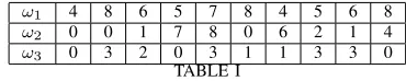
TABLE I
EXPECTED DEMAND FOR THE UPCOMING TEN DAYS.
C. The NDP Algorithm
This Algorithm is organized in two parts. In the first part
the retailers compute the set of admissible decisions Uk
i
and reachable statesRk
i over the horizon. The second part
presents three steps.
1) Policy improvement. For given prediction Ψ, we im-prove the policy via the stochastic Bellman’s equation backwards in time
µki(I k
i) =argminuk
i∈U
k
i(x
k i)
gi(Iik, u k i, k)
+αk+1ψ
ak•Jbi
k+1
(Iik+1,•)i.
2) Value iteration. The improved policy is valued through repeated Quasi-Monte Carlo simulations. Ac-tive exploration guarantees that initial states are suf-ficiently spread over the local minima. During the value iteration we compute and store the number of times a transitionΨijoccurs during the repeated finite
length simulations. At the end of each simulation, the protocol runs over the horizon and returns the training set for the next step.
3) Temporal Difference. We use the training set to update the transition probabilities of the predictor.
The tree steps are iteratively repeated until convergence of policies.
Lemma 4.1: Each iteration of the NDP algorithm, for
given initial state x0, has computational complexity
poly-nomial on the number of retailers, i.e.,O(n2N R2)
Proof: The proof starts from considering that the complexity of the algorithm depends essentially on the complexity of the second part. Here, we write the Bellman’s
equation considering the set of feasible decisions Uk
i, for
each retaileri∈Γ, for each stage k= 1,2, ..., N and for
each decomposed stateIk
i ∈(Rki×Γ). Thus, complexity is
O(n2N R2).
Assuming that convergence is achieved in a finite number of iterations, the Temporal Difference Algorithm returns stochastic Nash equilibrium policies, paths and costs-to-go. Further efforts are still to be made, oriented to investigate the convergence conditions of this algorithm.
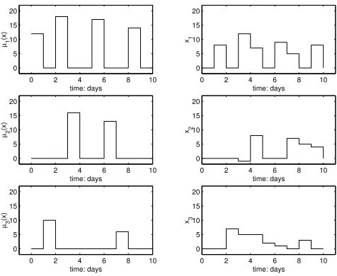
Example 1: Let us consider a group of three retailers and
parameters K = 24, p= 8, h = 1, and c = 2. Retailers
face a stochastic poissonian demand with expected values over the horizon of ten days as in Table I.
At the first iteration, no communication has occurred among the retailers and the “policy improvement” returns the uncoordinated reordering policies displayed in Fig. 7.
The “value iteration” consists in 12 simulations of the
0 2 4 6 8 10 0
5 10 15 20
time: days µ1
(x)
0 2 4 6 8 10
0 5 10 15 20
time: days
x1
0 2 4 6 8 10
0 5 10 15 20
time: days
x2
0 2 4 6 8 10
0 5 10 15 20
time: days
x3
0 2 4 6 8 10
0 5 10 15 20
time: days µ2
(x)
0 2 4 6 8 10
0 5 10 15 20
time: days µ3
[image:7.612.60.298.70.265.2](x)
Fig. 7. Uncoordinated reordering policies.
The set of initial states is a stochastic sequence extracted from a poissonian distribution with mean value respectively, equal to 25, 10, and 6 for the 1st, 2nd, and 3rd retailer. Indeed, we know from deterministic simulation results that
J1has potential local minima at18,23,30,J2at1,8,16,
and J3 at8,10 as displayed in Figure 9 (solid and dotted
lines). Here, the costs associated to the1st,2nd,3rd and4th policy improvements when demand is deterministic are rep-resented by four lines of different colors (blue, red, magenta, and red). At the end of each simulation the retailers run a
consensus protocol returning ak over the horizon. Based
on this new aggregate information, during the “temporal difference” the retailers update the transition probabilities of the predictor and a new iteration starts. In this example, the algorithm eventually converges to a Nash equilibrium in six iterations returning a coordinated distribution of reorders over the horizon as shown in Fig. 8. We see from Fig. 9
0 2 4 6 8 10
0 5 10 15 20
time: days µ1
(x)
0 2 4 6 8 10
0 5 10 15 20
time: days
x1
0 2 4 6 8 10
0 5 10 15 20
time: days
x2
0 2 4 6 8 10
0 5 10 15 20
time: days
x3
0 2 4 6 8 10
0 5 10 15 20
time: days µ2
(x)
0 2 4 6 8 10
0 5 10 15 20
time: days µ3
[image:7.612.320.543.146.318.2](x)
Fig. 8. Coordinated reordering policies.
that the costs-to-go at the 4th and 5th iteration (green
and red crosses) draw much near to the cost-to-go of the deterministic problem. We may conclude that the NDP algorithm possesses satisfying learning capabilities.
−100 0 10 20 30 40 50 60
500 1000 1500
x
J(x)
−100 0 10 20 30 40 50 60
200 400 600 800
x
J(x)
−100 0 10 20 30 40 50 60
200 400 600
x
J(x)
Fig. 9. Costs vs inventory: deterministic (colored lines) and stochastic demand (colored crosses).
V. CONCLUSION
In this paper we propose an NDP approach to coordinate the reordering policies of a group of retailers. Coordination is motivated by the possibility of sharing set up cost when orders are placed in conjunction. We develop a hybrid model to describe the inventory subsystems and the information flow. We designed consensus protocols for the information flow. Finally we presented a scalable and suboptimal NDP algorithm.
REFERENCES
[1] S. Axs¨ater, “A framework for decentralized multi-echelon inventory control”,IIE Transactions, vol. 33, no. 1, 2001, pp. 91-97. [2] D. Bauso, “Cooperative Control and Optimization: a Neuro-Dynamic
Programming Approach”,Ph. D. ThesisUniversit`a di Palermo, Dipar-timento di Ingegneria dell’Automazione e dei Sistemi, Dec. 2003. [3] D. Bauso and L. Giarr`e and R. Pesenti, “Distributed Consensus
Protocols for Coordinating Buyers”, Proc. of the IEEE Conference on Decision and Control, Maui, Hawaii, Dec. 2003.
[4] D. P. Bertsekas,Dynamic Programming and Optimal Control, 2nd ed. Bellmont, MA: Athena, 1995.
[5] D. P. Bertsekas and J. N. Tsitsiklis,“Neuro-Dynamic Programming”,
Athena Scientific, Bellmont, MA, 1996.
[6] J. C. Fransoo, M. J. F. Wouters and T. G. de Kok, “Multi-echelon multi-company inventory planning with limited information exchange”,Journal of the Operational Research Society, vol. 52, no. 7, Jul. 2001, pp. 830-838.
[7] R. Olfati Saber and R. M. Murray, “Consensus Protocols for Networks of Dynamic Agents”,Proc. of American Control Conference, Denver, Colorado, Jun. 2003.
[8] H. E. Scarf, “Inventory Theory”,Operations Research, vol.50, no.1, Jan-Feb 2002, pp.189-191.
[9] H. E. Scarf, “The Optimality of (s, S) Policies in the Dynamic Inventory Problem”, Mathematical Methods in the Social Sciences, Stanford University Press, Stanford, CA, 1995.
[10] Z. Yu, H. Yan and T. C. E. Cheng, “Modelling the benefits of information sharing-based partnerships in a two-level supply chain”,
[image:7.612.60.304.531.724.2]