On the Calculation of Dynamic Derivatives Using
Computational Fluid Dynamics
Thesis submitted in accordance with the requirements of the University of Liverpool for the degree of Doctor in Philosophy
by
Andrea Da Ronch
M.Sc. [Aeronautics], Politecnico di Milano (Italy) and Royal Institute of Technology (Sweden), 2008 B.E. [Aerospace], Politecnico di Milano (Italy), 2006
Copyright ©2012 by Andrea Da Ronch
Abstract
In this thesis, the exploitation of computational fluid dynamics (CFD) methods for the flight dynamics of manoeuvring aircraft is investigated. It is demonstrated that CFD can now be used in a reasonably routine fashion to generate stability and control databases. Different strategies to create CFD-derived simulation models across the flight envelope are explored, ranging from combined low-fidelity/high-fidelity methods to reduced-order modelling.
For the representation of the unsteady aerodynamic loads, a model based on aero-dynamic derivatives is considered. Static contributions are obtained from steady-state CFD calculations in a routine manner. To more fully account for the aircraft motion, dynamic derivatives are used to update the steady-state predictions with additional contributions. These terms are extracted from small-amplitude oscillatory tests. The numerical simulation of the flow around a moving airframe for the prediction of dy-namic derivatives is a computationally expensive task. Results presented are in good agreement with available experimental data for complex geometries. A generic fighter configuration and a transonic cruiser wind tunnel model are the test cases. In the pres-ence of aerodynamic non-linearities, dynamic derivatives exhibit significant dependency on flow and motion parameters, which cannot be reconciled with the model formula-tion. An approach to evaluate the sensitivity of the non-linear flight simulation model to variations in dynamic derivatives is described.
The use of reduced models, based on the manipulation of the full-order model to re-duce the cost of calculations, is discussed for the fast prediction of dynamic derivatives. A linearized solution of the unsteady problem, with an attendant loss of generality, is inadequate for studies of flight dynamics because the aircraft may experience large excursions from the reference point. The harmonic balance technique, which approxi-mates the flow solution in a Fourier series sense, retains a more general validity. The model truncation, resolving only a small subset of frequencies typically restricted to include one Fourier mode at the frequency at which dynamic derivatives are desired, provides accurate predictions over a range of two- and three-dimensional test cases. While retaining the high fidelity of the full-order model, the cost of calculations is a fraction of the cost for solving the original unsteady problem.
aerodynamic derivatives when applied to conditions of practical interest (transonic speeds and high angles of attack). There is a definite need for models with more re-alism to be used in flight dynamics. To address this demand, various reduced models based on system-identification methods are investigated for a model case. A non-linear model based on aerodynamic derivatives, a multi-input discrete-time Volterra model, a surrogate-based recurrence-framework model, linear indicial functions and radial basis functions trained with neural networks are evaluated. For the flow conditions con-sidered, predictions based on the conventional model are the least accurate. While requiring similar computational resources, improved predictions are achieved using the alternative models investigated.
Acknowledgements
I would like to acknowledge my supervisors Profs. K. J. Badcock and G. N. Barakos. I would also like to extend my thanks to Dr. M. Ghoreyshi, now at USAF Academy, and all the colleagues, both past and present, in the Computational Fluid Dynamics Laboratory at the University of Liverpool for fruitful discussions and for creating a stimulating working environment over the past three years.
I particularly wish to thank Prof. K. J. Badcock who has been a great mentor and an example of continuous inspiration. His encouragement and ideas were of utmost help to this work and are very much appreciated. Last, but not least, my family shall not be forgotten for their support and patience.
Declaration
I confirm that the thesis is my own work, that I have not presented anyone else’s work as my own and that full and appropriate acknowledgement has been given where reference has been made to the work of others.
List of Publications
Refereed Journals
Da Ronch, A., Vallespin, D., Ghoreyshi, M., and Badcock, K. J., ”Evaluation of Dynamic Derivatives Using Computational Fluid Dynamics,” AIAA Journal, 2012; 50(2): 470–484. doi: 10.2514/1.J051304.
Da Ronch, A., Ghoreyshi, M., and Badcock, K. J., ”On the Generation of Flight Dynamics Aerodynamic Tables by Computational Fluid Dynamics,” Progress in Aerospace Sciences, 2011; 47(8): 597–620. doi: 10.1016/j.paerosci.2011.09.001.
Da Ronch, A., McCracken, A., Badcock, K. J., Widhalm, M., and Campobasso, M. S., ”Linear Frequency Domain and Harmonic Balance Predictions of Dynamic Derivatives,” submitted to Journal of Aircraft, 2011.
Vallespin, D., Da Ronch, A., Badcock, K. J., and Boelens, O., ”Validation of Vortical Flow Predictions for a UCAV Wind Tunnel Model,” Journal of Aircraft, 2011; 48(6): 1948–1959. doi: 10.2514/1.C031385.
Ghoreyshi, M., Badcock, K. J., Da Ronch, A., Vallespin, D., and Rizzi, A., ”Auto-mated CFD Analysis for the Investigation of Flight Handling Qualities,” Mathematical Modelling of Natural Phenomena, 2011; 6(3): 166–188. doi: 10.1051/mmnp/20116307.
Ghoreyshi, M., Badcock, K. J., Da Ronch, A., Marques, S., Swift, A., and Ames, N., ”Framework for Establishing the Limits of Tabular Aerodynamic Models for Flight Dynamics Analysis,” Journal of Aircraft, 2011; 48(1): 42–55. doi: 10.2514/1.C001003.
Vallespin, D., Badcock, K. J., Da Ronch, A., White, M., Perfect, P., and Ghoreyshi, M., ”Computational Fluid Dynamics Framework for Aerodynamic Model Assessment,” to appear in Progress in Aerospace Sciences, 2012.
47(8): 674–694. doi: 10.1016/j.paerosci.2011.05.002.
Richardson, T., McFarlane, C., Isikveren, A., Badcock, K. J., and Da Ronch, A., ”Analysis of Conventional and Asymmetric Aircraft Configurations Us-ing CEASIOM,” Progress in Aerospace Sciences, 2011; 47(8): 647–659. doi: 10.1016/j.paerosci.2011.08.008
Richardson, T., Beaverstock, C., Isikveren, Meheri, A., Badcock, K. J., and Da Ronch, A., ”Analysis of the Boeing 747–100 Using CEASIOM,” to appear in Progress in Aerospace Sciences, 2011; 47(8): 695–705. doi: 10.1016/j.paerosci.2011.08.009
Badcock, K. J., Timme, S., Marques, S., Khodaparast, H., Prandina, M., Mottershead, J. E., Swift, A., Da Ronch, A., and Woodgate, M., ”Transonic Aeroelastic Simulation for Envelope Searches and Uncertainty Analysis,” Progress in Aerospace Sciences, 2011; 47(5): 392–423. doi: 10.1016/j.paerosci.2011.05.002.
Papers in Conference Proceedings
Da Ronch, A., McCracken, A., Badcock, K. J., Ghoreyshi, M., and Cummings, R. M., ”Modeling of Unsteady Aerodynamic Loads,” AIAA–2011–2376, AIAA Atmospheric Flight Mechanics Conference, Portland, Oregon, 8–11 Aug 2011.
Da Ronch, A., Ghoreyshi, M., Vallespin, D., Badcock, K. J., Mengmeng, Z., Op-pelstrup, J., and Rizzi, A., ”A Framework for Constrained Control Allocation Using CFD-based Tabular Data,” AIAA–2011–925, 49th AIAA Aerospace Sciences Meeting and Exhibit, Orlando, Florida, 4–7 Jan 2011.
Da Ronch, A., McFarlane, C., Beaverstock, C., Oppelstrup, J., Mengmeng, Z., and Rizzi, A., ”Benchmarking CEASIOM Software to Predict Flight Control and Flying Qualities of the B–747,” ICAS 2010–282, Proceedings of the 27th Congress of the In-ternational Council of the Aeronautical Sciences, Nice, France, 19–24 Sep, 2010.
Mialon, B., Khrabrov, A., Da Ronch, A., Cavagna, L., Mengmeng, Z., and Ricci, S., ”Benchmarking the Prediction of Dynamic Derivatives: Wind Tunnel Tests, Val-idation, Acceleration Methods,” AIAA–2010–8244, AIAA Guidance, Navigation and Control Conference, Toronto, Canada, 2–5 Aug, 2010.
Ghoreyshi, M., Vallespin, D., Badcock, K. J., Da Ronch, A., Vos, J. B., and Hitzel, S., ”Flight Manoeuvre Validation of Data Tables Generated Using an Aerodynamic Model Hierarchy,” AIAA–2010–8239, AIAA Guidance, Navigation and Control Conference, Toronto, Canada, 2–5 Aug, 2010.
Eliasson, P., Vos, J. B., Da Ronch, A., Mengmeng, Z., and Rizzi, A., ”Virtual Aircraft Design of TransCRuiser – Computing Break Points in Pitch Moment Curve,” AIAA– 2010–4366, 28th AIAA Applied Aerodynamics Conference, Chicago, IL, 28 Jun–1 Jul, 2010.
Vallespin, D., Da Ronch, A., Boelens, O., and Badcock, K. J., ”Validation of Vorti-cal Flow Predictions for a UCAV Wind Tunnel Model,” AIAA–2010–4560, 28th AIAA Applied Aerodynamics Conference, Chicago, IL, 28 Jun–1 Jul, 2010.
Da Ronch, A., Badcock, K. J., Ghoreyshi, M., G¨ortz, S., Widhalm, M., Dwight, R., and Campobasso, S., ”Linear Frequency Domain and Harmonic Balance Predictions of Dynamic Derivatives,” AIAA–2010–4699, 28th AIAA Applied Aerodynamics Confer-ence, Chicago, IL, 28 Jun–1 Jul, 2010.
Da Ronch, A., Vallespin, D., Ghoreyshi, M., and Badcock, K. J., ”Computation and Evaluation of Dynamic Derivatives using CFD,” AIAA–2010–4817, 28th AIAA Applied Aerodynamics Conference, Chicago, IL, 28 Jun–1 Jul, 2010.
Ghoreyshi, M., Badcock, K. J., Da Ronch, A., Swift, A., Marques, S., and Ames, N., ”Framework for Establishing the Limits of Tabular Aerodynamic Models for Flight Dy-namics,” AIAA–2009–6273, AIAA Atmospheric Flight Mechanics Conference, Chicago, IL, 10–13 Aug 2009.
Ghoreyshi, M., Da Ronch, A., Badcock, K. J., Dees, J., Berard, E., and Rizzi, A., ”Aerodynamic Modelling for Flight Dynamics Analysis of Conceptual Aircraft De-signs,” AIAA–2009–4121, 27th AIAA Applied Aerodynamics, San Antonio, Texas, 22– 25 Jun 2009.
Rizzi, A., Grabowski, T., Vos, J., Mieszalski, D., Da Ronch, A., Tomac, M., and Ghoreyshi, M., ”Creating Aero-Databases by Adaptive-Fidelity CFD Coupled with S&C Analysis to Predict Flying Qualities,” Paper in Special Technology Session, CEAS Paper, Manchester, UK, 26–29 Oct 2009.
Presentations without Proceedings
Technical Reports
Table of Contents
Abstract 5
Acknowledgements 7
Declaration 9
List of Publications 11
List of Figures 19
List of Tables 25
List of Symbols 27
1 Introduction 31
1.1 Example Applications of CFD . . . 33
1.2 Predictive Aerodynamic Models . . . 34
1.2.1 Linear and Non-linear Indicial Functions . . . 34
1.2.2 Regression Models . . . 35
1.2.3 Radial Basis Functions Interpolation . . . 36
1.2.4 Volterra Theory . . . 36
1.2.5 Proper Orthogonal Decomposition . . . 37
1.2.6 Surrogate-Based Models . . . 38
1.3 Review of Dynamic Derivatives . . . 38
1.4 Thesis Outline . . . 40
2 Formulation 43 2.1 Introduction . . . 43
2.2 Nonlinear Quasi-Steady Aerodynamic Model . . . 44
2.3 Kriging-Based Framework . . . 46
2.3.1 Initial Sampling . . . 47
2.3.2 Kriging Interpolation . . . 47
2.3.3 Iterative Sampling . . . 49
2.4 Hierarchy of Aerodynamic Models . . . 51
2.4.1 Semi-Empirical Method . . . 51
2.4.2 Linear Potential Solver . . . 52
2.5 CFD Flow Solver . . . 52
2.5.1 PMB (University of Liverpool) . . . 52
2.5.2 TAU (German Aerospace Center) . . . 54
2.5.3 COSA (University of Glasgow) . . . 55
2.5.4 Cobalt . . . 55
2.6 Calculation of Dynamic Derivatives . . . 56
3 Dynamic Derivatives from Unsteady Time-Domain CFD Simulations 61 3.1 Introduction . . . 61
3.2 Test Cases . . . 62
3.2.1 Standard Dynamic Model Aircraft . . . 62
3.2.2 Transonic CRuiser Wind Tunnel Model . . . 64
3.3 Numerical Results . . . 65
3.3.1 Standard Dynamic Model Aircraft . . . 66
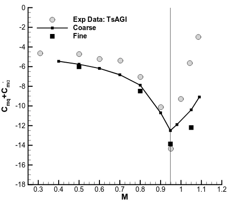
3.3.1.1 Mach Number . . . 67
3.3.1.2 Mean Angle of Incidence . . . 70
3.3.1.3 Reduced Frequency . . . 75
3.3.1.4 Oscillatory Amplitude . . . 79
3.3.1.5 Large Amplitude Motions . . . 80
3.3.2 Transonic CRuiser Wind Tunnel Model . . . 82
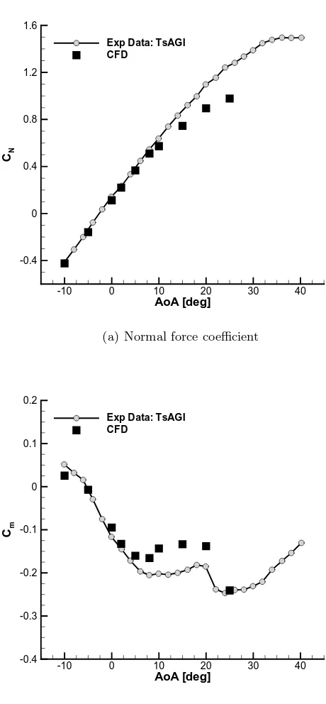
3.3.2.1 Static Cases . . . 84
3.3.2.2 Small Amplitude Motions . . . 85
3.3.2.3 Large Amplitude Motions . . . 88
3.4 Conclusions . . . 93
4 Dynamic Derivatives from Frequency-Domain Methods 95 4.1 Introduction . . . 95
4.1.1 Harmonic Balance Method . . . 96
4.1.2 Small Disturbance Method . . . 97
4.2 Frequency-Domain Methods . . . 99
4.2.1 Harmonic Balance Method . . . 99
4.2.2 Linear Frequency Domain Method . . . 101
4.2.3 Method of Data Analysis . . . 102
4.3 Two-Dimensional Case . . . 103
4.3.1 Numerical Setup . . . 103
4.3.2 Validation . . . 104
4.3.3 Frequency-Domain Results . . . 109
4.4 Three-Dimensional Case . . . 118
4.4.1 Numerical Setup . . . 118
4.4.2 Results . . . 119
4.5 Conclusions . . . 122
5 Reduced Models for Flight Dynamics 125 5.1 Introduction . . . 125
5.2 Two-Dimensional Case . . . 126
5.2.1 Numerical Setup . . . 126
5.2.2 Validation . . . 127
5.2.3 Large Amplitude Manoeuvre . . . 128
5.3 Model Formulation . . . 129
5.3.1 Volterra Series . . . 130
5.3.2 Surrogate-Based Recurrence-Framework . . . 132
5.3.3 Indicial Function . . . 133
5.3.4 Radial Basis Function . . . 134
5.4 Numerical Results . . . 134
5.4.1 Model based on Aerodynamic Derivatives . . . 134
5.4.2 Volterra Series . . . 137
5.4.3 Surrogate-Based Recurrence-Framework . . . 139
5.4.4 Indicial Function and Radial Basis Function . . . 142
5.5 Model Evaluation . . . 143
5.6 Conclusions . . . 145
6 Conclusions and Outlook 147 Bibliography 153 A Applications to Flight Dynamics 171 A.1 Transonic CRuiser Model . . . 171
A.2 Asymmetric Aircraft Model . . . 177
A.3 DLR-F12 Model . . . 180
A.4 Large Transport Civil Aircraft Model . . . 186
A.5 Standard Dynamic Model . . . 193
A.6 Ranger 2000 Aircraft . . . 196
A.7 Conclusions . . . 201
B Applications of Indicial Aerodynamics 203 B.1 Formulation . . . 204
B.2 Validation . . . 205
B.3 Prediction . . . 210
List of Figures
3.1 SDM layout [125] . . . 62
3.2 Surface grid for the SDM model geometry [131] . . . 63
3.3 Viscous grid of TCR wind tunnel model [131] . . . 64
3.4 Chordwise grid section on the wing . . . 65
3.5 Pitching moment coefficient loops for the SDM model geometry at two values of Mach number; the term ”tsc” indicates the number of physical time steps per cycle of unsteadiness . . . 68
3.6 Influence of Mach number on the pitch damping derivative for the SDM model geometry; experimental data were obtained in TsAGI [134] . . . . 68
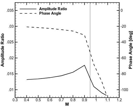
3.7 Amplitude ratio,R(¯ω), and phase angle,φ(¯ω), between the fundamen-tal harmonic of the angle of attack and the fundamenfundamen-tal harmonic of pitching moment coefficient; ¯ω indicates the oscillatory frequency of the applied forced motion . . . 70
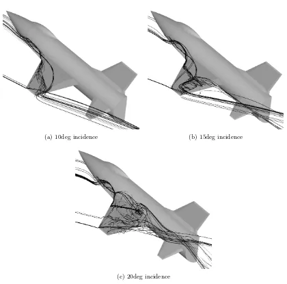
3.8 Flow field visualization for the SDM model geometry at Mach number of 0.3 . . . 71
3.9 Fixed-geometry unsteady calculations for the SDM model geometry at a Mach number of 0.3 and angle of attack of twenty degrees; the term ”ts” indicates the number of real time steps; horizontal thick lines mark the variation obtained in forced motion of five degrees amplitude for the half-fine grid . . . 72
3.10 Influence of mean angle of attack on the damping derivatives for the SDM model geometry at Mach number 0.3; experimental data were obtained in IHU [128] and AWT [129] . . . 74
3.13 Time history of pitching moment coefficient and phase lag in aerody-namic loads as a function of the reduced frequency; in (a), α0 = 15.0◦
and αA = 5.0◦; in (b), the mean angle of attack is ten degrees . . . 77
3.14 Influence of reduced frequency on the damping derivatives for the SDM geometry model at Mach number 0.3 (αA = 5.0◦); experimental data
were obtained in IHU [128] and AWT [129] . . . 78
3.15 Pitching moment coefficient loop for the SDM geometry model for the coarse grid at Mach number 0.3 and several values of the amplitude of motion, αA . . . 79
3.16 Influence of amplitude on the damping derivatives for the SDM geom-etry model at Mach number 0.3; experimental data were obtained in IHU [128] and AWT [129] . . . 81
3.17 Non-linear mathematical model and unsteady CFD for a large amplitude manoeuvre (α0 = 10.0◦,αA = 10.0◦ andk = 0.0493); (a) and (b) show
the small amplitude effects on the stability derivatives; (c) and (d) show the frequency effects . . . 83
3.18 Differences between time-accurate and time-averaged solutions of local contributions to the normal force coefficient; the axis of rotation is illus-trated . . . 84
3.19 Static longitudinal aerodynamic characteristics for the TCR wind tunnel model (M = 0.117 and Re = 0.778×10⁶) . . . 86
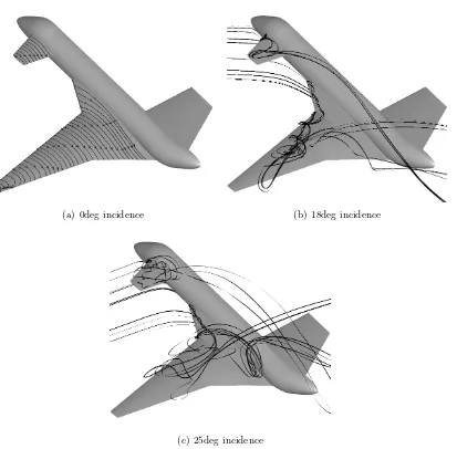
3.20 Surface streamlines and flow field visualization of the TCR wind tunnel model at several angles of attack . . . 87
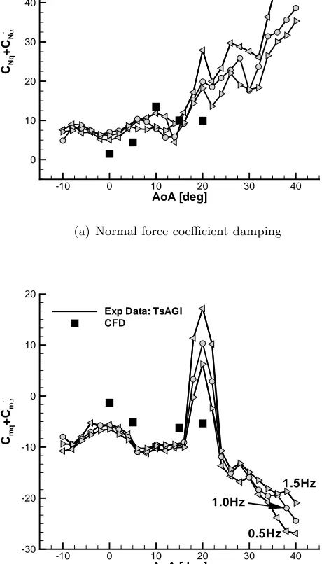
3.21 Damping derivatives for the TCR wind tunnel model (αA = 3.0◦); (a)
and (b) show the dependence on mean angle of attack (left triangles, f = 0.5Hz; circles, f = 1.0Hz; right triangles, f = 1.5Hz) . . . 89
3.22 Influence of frequency on the damping derivatives for the TCR wind tunnel model at mean angle of attack of ten degrees . . . 90
3.23 Dynamic dependencies for the TCR wind tunnel model for a large am-plitude manoeuvre (α0 = 8.0◦, αA = 10.0◦ and f = 1.0Hz) . . . 91
3.24 Mathematical model based on aerodynamic stability derivatives from wind tunnel (top) and CFD (bottom) simulations for the prediction of a large amplitude manoeuvre (α0 = 8.0◦,αA = 10.0◦ andf = 1.0Hz) 93
4.1 Grid used for the NACA 0012 aerofoil, medium grid (212×51) . . . 105
4.2 NACA 0012: predictions of unsteady time-accurate Euler solutions (M = 0.755,α0 = 0.016◦,αA = 2.51◦, and k = 0.0814); experimental
4.3 Instantaneous pressure coefficient distribution compared to experimental data of Landon [173]; the terms up and down in parenthesis indicate the direction increasing and decreasing angle, respectively (continued) . . . 107
4.4 Instantaneous pressure coefficient distribution compared to experimental data of Landon [173]; the terms up and down in parenthesis indicate the direction increasing and decreasing angle, respectively (concluded) . . . 108
4.5 NACA 0012: influence of amplitude of oscillatory motion, αA, on the
pitching moment coefficient dynamic derivatives (M = 0.755, α0 =
0.016◦
, andk = 0.0814) . . . 110
4.6 NACA 0012: normal force and pitching moment coefficients dynamic dependence (M = 0.755,α0 = 0.016◦,αA = 2.51◦, and k = 0.0814) . 111
4.7 NACA 0012: zeroth and first harmonic unsteady surface pressure co-efficient distribution (M = 0.755, α0 = 0.016◦, αA = 2.51◦, and
k = 0.0814) . . . 113
4.8 NACA 0012: magnitude and phase of pitching moment coefficient (M = 0.755, α0 = 0.016◦,αA = 2.51◦, and k = 0.0814) . . . 115
4.9 NACA 0012: CPU time speed up of the frequency-domain methods with respect to the underlying time-domain method; ”Nr Har” indicates the number of harmonics . . . 116
4.10 NACA 0012: error norm in the prediction of the damping-in-pitch ob-tained using the PMB solver pair; in (b), the term tsc indicates the number of time steps per cycle . . . 117
4.11 Structured and unstructured grids for the DLR-F12 model [182] . . . 119
4.12 DLR-F12 model: normal force and pitching moment coefficients dynamic dependence (M = 0.73, α0 = 0.70◦, αA = 0.50◦, k = 0.034, and
h = 6000m) . . . 120
4.13 DLR-F12 model: zeroth and first harmonic unsteady surface pressure coefficient distribution at Y /s = 0.148 (M = 0.73, α0 = 0.70◦, αA =
0.50◦
,k = 0.034, and h = 6000m) . . . 123
5.1 Viscous grids used for the NACA 0012 aerofoil . . . 127
5.2 NACA 0012: predictions of unsteady time-accurate viscous solutions (M = 0.6,α0 = 3.16◦,αA = 4.59◦,k = 0.0811, and Re = 4.8×10⁶);
experimental data from Landon [173] . . . 128
5.3 NACA 0012: unsteady time-accurate viscous solutions for the manoeu-vre to be predicted (M = 0.764, α0 = 0.0◦, αA = 8.5◦, k = 0.0811,
5.4 Dynamic derivatives for the NACA 0012 aerofoil (M = 0.764 andα0 =
0.0◦
); in (a)-(b), k = 0.10 and several values of amplitude; in (c)-(d), αA = 0.1◦and several values of reduced frequency; in (e)-(d),αA = 5.0◦
and several values of reduced frequency . . . 136
5.5 Non-linear mathematical model and unsteady CFD for a large amplitude manoeuvre (M = 0.764, α0 = 0.0◦, αA = 8.5◦, and k = 0.10); in
(a)-(b), dependence on the oscillatory amplitude at reduced frequency k = 0.10; in (c)-(d), dependence on the reduced frequency at oscillatory amplitude αA = 0.1◦; in (e)-(f), dependence on the reduced frequency
at oscillatory amplitudeαA = 5.0◦ . . . 138
5.6 NACA 0012: predictions of pitching moment dynamic dependence (M = 0.764, α0 = 0.0◦, αA = 8.5◦, and k = 0.10); ”Model” refers to the
discrete-time multi-input Volterra model . . . 139
5.7 Response surfaces of the time evolution of aerodynamic coefficients throughout the parameter space of oscillatory amplitude, αA (M =
0.764, α0 = 0.0◦, and k = 0.10); the solid curve indicates the
solu-tion at an amplitude of 5 deg . . . 140
5.8 Aerodynamic coefficients dynamic dependence for several value of oscil-latory amplitude (M = 0.764, α0 = 0.0◦, and k = 0.10); curves are
plotted every one-degree increment in amplitude . . . 141
5.9 Model predictions and unsteady CFD for a large amplitude manoeuvre (M = 0.764, α0 = 0.0◦,αA = 8.5◦, and k = 0.10); ”Model” refers to
the surrogate-based recurrence-framework . . . 142
5.10 NACA 0012: indicial responses of pitching moment coefficient to step change in angle of attack and in pitch rate (M = 0.764 andRe = 3.0×10⁶)143
5.11 NACA 0012: predictions of pitching moment dynamic dependence (M = 0.764, α0 = 0.0◦, αA = 8.5◦, k = 0.10, and Re = 3.0×10⁶); in (a),
”Model” refers to the linear indicial functions, and in (b) to radial basis functions . . . 144
A.1 Mission profile for the TCR configuration . . . 172
A.2 Wind-tunnel testing of the TCR model in TsAGI [148] . . . 172
A.3 TCR wind tunnel model; in (a), flow development computed using the PMB solver at 18◦
angle of attack at low speed; in (b), canard deflections of ±10◦
on a grid for use with the EDGE solver . . . 173
A.5 Distribution of low- and high-fidelity calculations in the two-dimensional parameter space of angle of attack and Mach number; the shaded area illustrates many solutions obtained using the linear potential method, TORNADO; CFD solutions were obtained at an ensemble of isolated points . . . 176
A.6 Baseline configuration representative of the EA500 Very Light Jet . . . 178 A.7 Asymmetric three-lifting surface configuration . . . 179
A.8 Wind-tunnel testings of the DLR-F12 model in DNW-NWB [200] . . . . 181 A.9 Different fidelity geometry representations of the DLR-F12 model; XML
and WT indicate, respectively, the low- and high-fidelity configurations; the elevator is highlighted in the XML geometry and the WT geometry has been mirrored to facilitate the geometry comparison . . . 182 A.10 Geometry increments to simulate a design study, featuring variation of
wing quarter-chord sweep angle, Λw, and wing area,S; the arrow points
at the wing tip trailing-edge of the baseline XML configuration, which represents the original XML design . . . 183
A.11 Trim conditions for the DLR-F12 full aircraft model at an altitude of 6000m comparing DATCOM and Euler solutions on the XML configu-ration and RANS solution on WT configuconfigu-ration . . . 185
A.12 Short-period and phugoid characteristics for the DLR-F12 full aircraft model at an altitude of 6000mcompared to ICAO recommendations [201]187 A.13 Impact of geometry increments in the short-period characteristics for the
DLR-F12 full aircraft model at an altitude of 6000m . . . 187
A.14 Overlay of a three-view of a B747 aircraft model and lifting surfaces for low-fidelity aerodynamics . . . 188
A.15 Medium-fidelity surface geometry for the B747-like model with control surfaces . . . 188
A.16 Variation of aerodynamic coefficients with angle of attach and rudder deflection at a Mach number of 0.9; the black cubes indicate sample points190 A.17 Illustration of the aerodynamic table for ailerons deflection; black cubes
indicate sample points . . . 190
A.18 Variable-fidelity aerodynamic predictions compared to experimental data at Mach number of 0.8 for the B747-like model; experimental data are from [204] . . . 191
A.19 Trim conditions at transonic speed range for the B747-like model at an altitude of 11000m using different fidelity aerodynamic models . . . 192
A.20 Deflected control surfaces for the SDM model . . . 193 A.21 Response of aerodynamic coefficients to angle of attach and elevator
A.22 Wing-over and a 90-degree turn manoeuvres were simulated for the SDM model in [23] . . . 196 A.23 A three-view of the Ranger 2000 aircraft . . . 196 A.24 Grid for the Ranger 2000 aircraft; the surface solution is obtained at
α = 6.0◦
and M = 0.8 . . . 197 A.25 Response of aerodynamic coefficients to angle of attach and Mach
num-ber at zero sideslip angle; the black cubes indicate sample points . . . . 198 A.26 Illustration of the aerodynamic tables for deflection of control surfaces
at a Mach number of 0.25; black squares indicate sample points . . . 199 A.27 Simulation of manoeuvres for the Ranger 2000 aircraft compared to flight
test data . . . 200
B.1 Indicial response of lift coefficient for a step change in angle of attack (∆α = 4.58◦
) . . . 206 B.2 Indicial response of lift coefficient for a step change in angle of attack for
small times (∆α = 4.58◦
); reference data are from Lomax [213] . . . 207 B.3 Indicial response of lift coefficient for a sharp-edged gust at Mach number
0.20 normalized by its asymptotic value (wg/U = 0.08) . . . 208
B.4 Indicial response of lift coefficient for a sharp-edged gust for small times (wg/U = 0.08); reference data are from Lomax [213] . . . 209
B.5 Indicial response of lift coefficient for a moving sharp-edged gust at Mach number 0.20 normalized by its asymptotic value (wg/U = 0.08); the
solution for λ = 1 is not plotted, see Fig. B.3 . . . 209 B.6 Lift dynamic dependence from unsteady CFD calculations and two
con-volution models in response to gust of different shapes; in (a), τg = 10
and wg/U = 0.08; in (b), τg = 25 and wg/U = 0.08; and in (c),
List of Tables
2.1 Aerodynamic database format [81]; ”x” indicates a column vector of non-zero elements . . . 45
3.1 Reference values of the SDM model geometry . . . 64
3.2 Reference values of the TCR wind tunnel model . . . 66 3.3 Description of the SDM test cases; terms in parentheses indicate
sec-ondary dependencies of the investigations . . . 67 3.4 Experimental conditions for testing of the TCR wind tunnel model at
TsAGI T–103 facility [148] . . . 84
4.1 Description of the AGARD CT5 conditions for the NACA 0012 aero-foil [173] . . . 103 4.2 NACA 0012: grid influence on static and dynamic derivatives obtained
from the time-domain PMB solution for the AGARD CT5 conditions . . 104 4.3 NACA 0012: amplitude ratio and phase angle of the fundamental
har-monic between the input,α, and the outputs, CN and Cm . . . 112
4.4 NACA 0012: normal force and pitching moment coefficient dynamic derivatives (M = 0.755,α0 = 0.016◦, αA = 2.51◦, and k = 0.0814) . . 114
4.5 NACA 0012: time reduction of the PMB-HB solution compared to un-steady PMB solution using the damping-in-pitch as the figure of merit; the termstscandnc indicate, respectively, the number of time-steps per
cycle and the number of oscillatory cycles . . . 118 4.6 Description of the conditions for the DLR-F12 aircraft model . . . 120 4.7 DLR-F12 model: normal force and pitching moment coefficient dynamic
derivatives (M = 0.73, α0 = 0.70◦, αA = 0.50◦, k = 0.034, and
h = 6000m) . . . 121
5.1 Description of the AGARD CT2 conditions for the NACA 0012 aero-foil [173] . . . 128 5.2 Error norm in the model predictions of pitching moment coefficient and
A.1 Reference values and mass and inertia properties of the TCR aircraft model . . . 176 A.2 Reference values and mass and inertia properties of the DLR-F12 full
aircraft model . . . 184 A.3 Reference values and mass and inertia properties of the B747-like model 192 A.4 Mass and inertia properties of the SDM model . . . 194 A.5 Reference values and mass and inertia properties of the Ranger 2000
aircraft . . . 197
List of Symbols
A = matrix in frequency domain equation
A = response to a step change function a = speed of sound, [m/s]
b = reference wing span, [m]
b0, b1, b2, b3 = coefficients in approximation to K¨ussner function for compressible flows
c = mean aerodynamic chord, [m] d = fuselage total length, [m] Cm = pitching moment coefficient
Cm0 = non-linear static pitching moment coefficient
Cmq + Cmα˙ = pitching moment coefficient damping, [1/rad]
CN = normal force coefficient
CN0 = non-linear static normal force coefficient
CNq + CNα˙ = normal force coefficient damping, [1/rad]
D = matrix in harmonic balance equation
F[ψ(t)] = Fourier transform of quantity ψ(t), equivalent to ˜ψ(j ω)
f = dimensional frequency, [Hz]
F[ψ(t)] = Fourier transform of quantity ψ(t), equivalent to ˜ψ(i ω)
G(iω) = transfer function of input/output pair
Hi =i-th order Volterra operator
Hi =i-th order Volterra kernel
H = response to a unit impulse function h = altitude, [m]
i = imaginary unit,√−1
k = reduced oscillation frequency, ω c/(2U∞) M∞ = freestream Mach number
nc = number of oscillatory cycles
nH = number of harmonics
R = residual vector
R(ω) = amplitude ratio of transfer function Re = Reynolds number,U∞c/ν
s = non-dimensional time used in analytical formulation, 2t U∞/c t = physical time, [s]
t∗
= non-dimensional time used in CFD, t U∞/c
ug, wg = horizontal and vertical velocity components of gust, [m/s]
Wg = gust vertical velocity function of time, [m/s]
U∞ = freestream speed, [m/s] W = vector of conserved variables
∠ψ˜(i ω) = phase angle of the Fourier transform of quantityψ(t)
Greek Symbols
α = angle of attack, [deg] α0 = mean angle of attack, [deg]
αA = amplitude of oscillatory motion, [deg]
β = angle of sideslip, [deg]
β1, β2, β3 = coefficients in approximation to K¨ussner function for compressible flows
ν = kinematic viscosity of air, [m2/s] φ(ω) = phase angle between output and input λ = advance ratio for gust
Φ = Wagner function
Ψ = K¨ussner function
Φ1,Φ2, ε1, ε2 = coefficients in Wagner function
Ψ1,Ψ2, ε3, ε4 = coefficients in K¨ussner function
τg = gust gradient
ω = oscillation frequency, 2π f, [rad/s]
Acronyms
CFD = computational fluid dynamics CFL = Courant–Friedrichs–Lewy number Cobalt = commercially available CFD solver COSA = CFD solver from University of Glasgow DLR = German Aerospace Center
EDGE = CFD solver from FOI
EIF = expected improvement function FOI = Swedish defence agency
F12 = large transport aircraft
HB = harmonic balance
LFD = linear frequency domain
MUSCL = monotonic upstream–centered scheme for conservation laws NSMB = Navier–Stokes multiblock
PMB = parallel multiblock
RANS = Reynolds–averaged Navier–Stokes RBF = radial basis function
ROM = reduced order model
SBRF = surrogate-based recurrence-framework SDM = standard dynamic model
TAU = CFD solver from DLR TCR = transonic cruiser
Chapter 1
Introduction
Determining the stability and control characteristics of aircraft at the edge of the en-velope is one of the most difficult and expensive aspects of the aircraft development process. Non-linearities and unsteadiness in the flow are associated with shock waves, separation, vortices and their mutual interaction, which can lead to uncommanded motion and uncontrollable departure. If these issues are discovered at flight test, the aircraft development can suffer significant delays, a rise in production costs and detri-mental effects on performance. There have been numerous examples of aircraft experi-encing uncommanded activity, as reported, for instance, in [1]. Following an extensive resolution process, immediate improvements are typically achieved by minor configura-tion changes and modificaconfigura-tions to the flight control system and control augmentaconfigura-tion laws. To provide a better fundamental understanding of the flow physics causing de-graded characteristics, computational approaches have been used [2]. The development of a reliable computational tool for prediction of these important issues would allow the designer to screen different configurations prior to building the first prototype, reducing overall costs and limiting risks [3].
A possible useful addition to the high-fidelity/high-cost of testing and low-fidelity/low-cost of semi-empirical approaches is Computational Fluid Dynamics (CFD), which represents the state of the art in predicting non-linear flow physics. Success has been reported in predicting the non-linear aerodynamic behaviour of air-craft at full scale Reynolds numbers [9]. However, the generality realized in a CFD simulation comes at the expense of computational cost. Due to the ”curse of dimen-sionality” (a term coined by Bellman [10]), routine use of high-fidelity CFD simulations is costly to cover a large parameter space of conditions, such as in multidisciplinary op-timization [11], aeroelasticity [12] and studies of flight dynamics [13]. The term fidelity here indicates the level of physical modelling realized in the numerical techniques used. High-fidelity analyses refer to mathematical models for the description of the relevant physics in the problem to be simulated.
To generate the aerodynamic database of forces and moments for the expected flight envelope, a large number of flow conditions for different aircraft control settings are required. Considering that the total number of table entries can be in the order of hundreds of thousands or even millions, the task to simulate aerodynamic loads for each single entry is extremely expensive, and is intractable using CFD as a source of the data. An alternative method to the ”brute-force” approach was presented in [14], and is based on the kriging interpolation [15,16], which is well suited to approximate non-linear functions [17, 18] and does not require a priori knowledge of the function to be approx-imated. While approximating the non-linear CFD results throughout the parameter space from a limited number of full-order simulations, the key to the methodology is the location of sample points. In addition to creating a high-fidelity aerodynamic database for improved predictions of the aircraft stability and control behaviour, CFD can be used to establish the limits of tabular models. The mathematical model typically used for flight dynamic investigations is based on the concept of stability or aerodynamic derivatives. Forces and moments are assumed to be a function of the instantaneous val-ues of the disturbance velocities, control angles and their rates [19]. Whilst consistent with a quasi-steady representation of the aerodynamics, the time-invariant assumption is questionable in many studies of unsteady aerodynamics [20]. Therefore, several at-tempts were made to improve the modelling of unsteady aerodynamic loads [21, 22]. The ability of CFD to perform unsteady simulations creates a framework for assessing the limits of the tabular model due to the neglect of time-history effects on the flow development. Various maneouvers were created in [23] solving an optimal-control prob-lem, and aerodynamic predictions obtained from the look-up tables were compared to the unsteady aerodynamic loads simulated from a time-accurate CFD analysis.
aerody-namic non-linearities are present. Alternative model formulations are evaluated, and advances in the prediction of non-linear unsteady aerodynamic loads are likely based on the results presented.
1.1
Example Applications of CFD
Progress made in reducing the time required to generate an aerodynamic database of forces and moments for a Harrier aircraft in ground effect was reported in [24]. With access to large-scale parallel computers, 35 time-dependent Reynolds-Averaged Navier-Stokes (RANS) simulations were completed in one week. A monotone cubic-spline interpolation procedure [25] was used to extend the 35 solution database to over 2500 cases for a range in angle of attack between 4◦
and 10◦
and in height above the ground between 10 and 30f t. A step towards the generation of a stability and control database to simulate take-off and landing scenarios for a YAV-8B Harrier was described in [26]. The aerodynamic model for the force and moment coefficients was expressed in terms of the static and dynamic stability derivatives. It was envisioned that a few hundred solutions could be obtained, and the remainder of the parameter space filled out with the use of an interpolation procedure or neural networks. A system to automate the process of running a large number of expensive CFD simulations on grid resources based on Globus [27] was developed, allowing the generation of one hundred RANS and one thousand Euler simulations in one week for a second generation Langley glide-back booster design [28]. The database of forces and moments was computed varying the angle of attack, Mach number and angle of sideslip, and was compared against experimental data.
influence of any dynamic derivatives. The databases were created from a set of discrete points at the minimum, median and maximum values for each independent parameter. While this approach drastically reduces the number of computations, it also presumes that these points capture all the relevant non-linearities in aerodynamic loads. Further tests were not reported to investigate the validity of this assumption.
1.2
Predictive Aerodynamic Models
The references cited above exemplify the need for improvements in computational effi-ciency. While access to high-end computing facilities is essential for numerous examples of intensive CFD simulations [31,32], to make progress in routinely using CFD, research has been concentrated on the development of computationally efficient predictive aero-dynamic models to use in combination with CFD generated data.
1.2.1 Linear and Non-linear Indicial Functions
Linearized aerodynamic models based on a functional representation for the indicial aerodynamic force and moment responses (see Appendix B) in terms of blade motion and gust functions were used in subsonic flow [33]. A method was developed to calculate the indicial and gust responses of an airfoil in compressible flow directly using CFD [34]. The step change was incorporated into an existing CFD solver using a grid-velocity ap-proach, and accurate solutions compared to exact analytical results were obtained at low speed. The agreement degraded with non-linear compressibility effects. The fi-delity of linearized indicial methods for aerodynamic load predictions was assessed, and it was found that these methods are sufficiently accurate to be used as a practical design tool [35]. However, simplifying assumptions from the flow physics limits the generality of the linear indicial approach. When non-linear effects are significant, such as when there is the appearance/disappearance of a shock wave or topological changes of the flow, the indicial approach becomes inaccurate [36]. In addition, flowfields with hysteresis exhibit memory-effects, which violate the assumption of time-invariance un-derlying the linear indicial approach.
demonstrated to accurately describe unsteady aerodynamic effects observed in experi-mental investigations [22]. The model extends the usual flight dynamics equations by introducing a first order delay differential equation for an additional internal state vari-able which accounts for unsteady effects associated with separated and vortical flow. It was claimed that an efficient parametrization of the indicial function space can be obtained based only on local information, such as instantaneous angle of attack and pitch rate. The non-linear indicial prediction model was also tested for a rectangular wing undergoing dynamic stall [40]. An artificial neural network trained on wind tun-nel data was used to reproduce the detailed aerodynamic characteristics of the pitching wing, and deemed accurate enough to provide a reference solution for the prediction model at negligible cost. In view of the mathematical formulation adopted in this work, it is significant that a comparison between the non-linear indicial method and the aerodynamic stability derivatives method was reported. First, a model with con-stant coefficient aerodynamic derivatives, retaining a quadratic term in angle of attack and expressing the damping derivative as a function of the angle of attack, was consid-ered. Constant coefficient derivatives were determined from the neural network using an identification technique. A second model using a look-up table for static aerody-namics, augmented with alpha-dependent damping derivatives, was built. Both models were used to predict aerodynamic loads for a constant pitch rate maneuver at a reduced frequency of 0.02, from zero up to sixty degrees angle of attack. It was demonstrated that the indicial method was significantly more accurate than the conventional model based on aerodynamic stability derivatives for the unsteady maneuver tested, particu-larly when critical states were crossed. It was concluded that efficient parametrization of the indicial and critical state function space appears to be achievable using only local information, such as the instantaneous angle of attack and pitch rate. The accuracy of the non-linear indicial method was also reported for the prediction of the airloads for a 65◦
delta wing performing forced roll oscillations at high angle of attack [41].
1.2.2 Regression Models
calculated with CFD. A reduced-order mathematical model is then built from the sim-ulated aerodynamic loads using system identification methods [47], and the prediction model is compared with the training maneuvers used to generate it. Finally, the predic-tion model is applied to novel maneuvers, and for the predicpredic-tion of aerodynamic loads at all flight test points at negligible cost. SIDPAC [48] has been a common choice to build reduced-order models [49]. It is a least squares regression based method that generates an explicit relationship between the computed aerodynamic loads and the independent variables of the aircraft motion. Unsteady time-accurate Delayed Detached-Eddy Sim-ulations (DDES) were calculated at a Mach number of 0.4, constant angle of attack of 30◦
and sinusoidally varying angle of sideslip. Five maneuvers were performed at constant frequency, and a chirp frequency maneuver was additionally performed for a frequency sweep between zero and 17Hz. To assess validity, the prediction model built from the chirp frequency motion was used to reproduce the aerodynamic loads for a maneuver at constant frequency included within the bounds of the training signal used to generate the model. It was demonstrated [44] that a regression model is incapable of generating an accurate low-order model of the airloads based on the analysis of one single training maneuver.
1.2.3 Radial Basis Functions Interpolation
The determination of an appropriate training maneuver is a challenging task, which is vital for the successful generation of a reduced-order model. Past research has focused on the development of training maneuvers, and used the frequency content and power spectral density of the motion variables as figures of merit [50, 51]. This approach is not always valid as the functional dependences relating the aerodynamic loads to the aircraft motion are far more complex. A different approach, based on the ability to cover the relevant regressor space and to capture a range of flow phenomena, was adopted for the investigation of training maneuvers for a two-dimensional airfoil [52]. Several training maneuvers, such as chirp, spiral and Schroeder maneuvers, were considered, and used to build reduced-order models. To assess the accuracy of the prediction models, aerodynamic loads were compared against time-accurate CFD solutions. The reduced order models were based on radial basis functions [53], and an improvement in the ability to predict linear and non-linear aerodynamic characteristics using one single training signal was observed. It was concluded that the chirp maneuver resulted in the most robust and reliable reduced order model, and the spiral maneuver was found adequate for low-frequency and static aerodynamic predictions.
1.2.4 Volterra Theory
aeroe-lastic studies of limit cycle oscillations [55, 56]. The extension into the area of stability and control was considered in [57]. Two test cases were evaluated, a NACA 0012 airfoil and a X-31 aircraft model. The Volterra kernels were identified from a set of Gaus-sian shaped impulses, and the accuracy of the prediction model for different pitching motions was assessed. The applications were limited to linear cases, and a good agree-ment of the Volterra reduced-order modeling was observed when compared to time-accurate CFD simulations in the linear aerodynamic range. With weakly non-linear characteristics, the performance of the prediction model quickly degraded. As stated in the review [56], an important issue is the excitation of multiple degrees of freedom to properly identify non-linear cross-coupling of the degrees of freedom, and because of the non-linear nature of the aerodynamic system the principle of superposition is invalid. A method for the inclusion of Volterra cross-kernels applied to a transonic two-dimensional airfoil undergoing forced pitch and plunge harmonic oscillations was investigated [58]. The prediction model was compared to time-accurate CFD solutions, and the improvement in accuracy over approaches that ignore the cross-kernels was demonstrated. Addressing the convergence issue of the Volterra series and the need for the inclusion of higher-order kernels, an alternative formulation was presented [59]. The pruned Volterra series, with a simplified parametric structure of the kernels, was tested for a two-dimensional transonic airfoil undergoing forced sinusoidal pitch oscillations for two AGARD test cases. The identification of kernels up to fourth order demon-strated a feasible undertaking and a good agreement compared to the time-accurate CFD solution was achieved. The formulation of the pruned Volterra series was then used to approximate the flutter boundary and limit-cycle oscillation amplitudes of the NACA 0012 benchmark model [60]. Showing favourable results, a computational saving of several orders of magnitude compared to full-order CFD simulations was achieved.
1.2.5 Proper Orthogonal Decomposition
solutions, e.g. snapshots, was identified as the most expensive task. Once the POD basis vectors were found, the construction and solution of the reduced-order model was done at negligible cost, making it suitable for parametric studies. Recent studies have been conducted to bring the POD theory in combination with standard identification methodologies in the analysis of maneuvering aircraft [64, 65]. A prescribed maneuver designed to densely populate a given flight parameter envelope was simulated with an unsteady CFD solver. The ensemble of snapshots used in the POD method consists of surface solutions taken at regular time increments. Time-dependent surface data were decomposed into a set of orthogonal modes in the spatial coordinate, and a set of time-dependent coefficients for each mode. The key for the described method is that the time-dependent coefficients are fitted to a polynomial function of the time histories of the relevant flight parameters. Once constructed, the model can be used to predict the surface data for an arbitrary maneuver, again at negligible cost compared to the full-order simulation.
1.2.6 Surrogate-Based Models
Despite the progress made in the development of reduced-order models, the selection of appropriate training data remains a key issue. The routine generation of reduced-order models has not been reported in any previous work. An alternative approach is based on surrogate modeling [66–68]. First described in [14], the framework builds on kriging interpolation [15, 16]. Note that the development of a similar framework applied to a two-dimensional airfoil restricted to one- and two-parameter variables was reported [69].
In addition to creating a high-fidelity aerodynamic database for improved predic-tions of the aircraft stability and control behaviour, CFD can be used to establish the limits of the tabular models. The mathematical model typically used for investiga-tions of flight dynamics is based on the concept of stability or aerodynamic derivatives. Forces and moments are assumed to be a function of the instantaneous values of the disturbance velocities, control angles and their rates [19]. Whilst consistent with a quasi-steady representation of the aerodynamics, these models cannot predict the non-linearities associated with post-stall aerodynamics, including bifurcations and hystere-sis. The ability of CFD to perform unsteady simulations allows the assessment of the limits of a tabular model arising from the neglect of time-history effects.
1.3
Review of Dynamic Derivatives
aerodynamic forces and moments are a function of the instantaneous values of the dis-turbance velocities, control angles and their rates. The dependence of the forces and moments on these variables is obtained by a Taylor series expansion, discarding higher order terms [70]. For slow motions at low angle of attack, the static derivatives are generally sufficient to model the aerodynamic loads [6]. At higher angles of attack and rates, the inclusion of dynamic derivatives in the aerodynamic model can have a significant effect on the calculated stability characteristics of an airframe [71]. The addition of non-linear terms to take into account changes of stability derivatives with the angle of attack extended the range of flight conditions to high angles of attack and/or high amplitude manoeuvres. In the linear and non-linear methods, it is as-sumed that the aerodynamic parameters are time invariant [47]. This assumption was often questioned based on many studies of unsteady aerodynamics [20]. In the 1920s, Wagner [72] conducted a series of studies for the unsteady lift generated on an airfoil due to abrupt changes in angle of attack. Theodorsen extended these studies investi-gating the forces and moments on an oscillating airfoil. The lift response of an airfoil penetrating sharp-edge and harmonically-varying gusts was studied by K¨ussner [73] and Sears [74], respectively. The first attempts to investigate unsteady aerodynamic effects on aircraft motion were made by Jones and Fehlner [75], studying the effect of the wing wake on the lift of the horizontal tail. A more general formulation of linear unsteady aerodynamics in the aircraft longitudinal equations of motion was introduced by Tobak [76]. Tobak and Schiff [21] replaced the indicial functions within the integrals with functionals [77], themselves dependent of the past motion. A different approach was proposed by Goman et al. [78] introducing additional state variables, named in-ternal state variables, in the functional relationships for the aerodynamic forces and moments. The coordinates of a separation point or vortex breakdown location can be taken as internal state variables, and modelled by differential equations. Goman and Khrabrov [22] formulated state space models with internal state variables describing the flow state. A good agreement was achieved with experimental data for a separated flow on an airfoil and flow with vortex breakdown about a slender delta wing.
motion as well as the interference effects of the model support are not factors in the computational analysis. Physical effects can be separated in the CFD solutions in a way which can be difficult from wind tunnel or flight test data. CFD can also be used for investigating the modelling of data from flight tests. There is of course a significant question about the ability of CFD to predict the relevant aerodynamics, and this must be demonstrated through validation studies. It is therefore possible to use CFD as a complement to costly experimental campaigns. However, CFD is not meant to replace testing techniques.
1.4
Thesis Outline
The work in this thesis was partly developed within the SimSAC (Simulating Aircraft Stability and Control Characteristics for Use in Conceptual Design) project 1 funded by the European Commission 6th Framework Programme. The project consisted of a partnership of European academics and industrial contributors. The main driver of the project was the inadequacy of standard semi-empirical approaches currently used in conceptual design when confronted with more advanced aircraft configurations [80]. This may cause errors in the design process, which may prove expensive to rectify via additional design work, wind tunnel and flight testing, in addition to a delay in certification and performance degradation. To overcome these potential issues, it is worthwhile to introduce high-fidelity (physics-based) approaches early in the design process.
In this thesis, the exploitation of CFD is investigated for the generation of the aero-dynamic database. A framework for the automated generation of tabular aeroaero-dynamic models for studies of flight dynamics is discussed, allowing stability and control con-siderations to be developed early in the design process. For the representation of the aerodynamic loads, a model based on stability or aerodynamic derivatives is assumed because traditionally used by flight dynamicists. In the model formulation, dynamic derivatives are used to update the static predictions to account for the aircraft motion. Emphasis is on the evaluation of dynamic derivatives with various CFD methods. As the limitations of the aerodynamic model are exposed for several test cases, there is a need for models of more realism and fidelity to be used in flight dynamics. Advances in this direction are discussed.
Chapter 2 introduces the framework for the generation of aerodynamic tables using CFD as the source of the data. The framework has been developed at Liverpool by the author and a colleague. A method to efficiently reduce the number of high-fidelity anal-yses is accomplished by use of a kriging-based surrogate model. Low-fidelity estimates are augmented with higher fidelity data, and data fusion combines the two datasets
1
into one single database. Once constructed, the look-up tables can be used in real-time to fly the aircraft through the database. Two methods for the evaluation of dynamic derivatives are also discussed.
Chapter 3 discusses the evaluation of dynamic derivatives computed using unsteady time-domain CFD simulations. Two configurations are considered: a generic fighter model and a transonic cruiser concept design. Numerical results are compared to experimental measurements, and a good agreement is noted in all cases. A systematic study to evaluate the dependencies of dynamic derivatives on aircraft motion and flow parameters, beyond the range of motions performed in dynamic testing facilities, is presented. It is recognized that in the presence of aerodynamic non-linearities, mainly due to three dimensional separated flow and concentrated vortices, dynamic derivatives exhibit a dependence on motion and flow parameters. These dependencies are not reconcilable with the model formulation, which is based on a Taylor series expansion. An approach to evaluate the sensitivity of the non-linear unsteady aerodynamic loads to variations in dynamic derivatives is introduced.
Chapter 4 introduces the use of reduced models, based on the manipulation of the full-order model, for the fast computation of dynamic derivatives. The underlying idea is to exploit the periodicity of the resulting aerodynamic system for oscillatory motions to decrease the cost of calculations. A linearized solution in the frequency domain and a harmonic balance technique are illustrated for two- and three-dimensional configurations. To stress the potential of the frequency-domain methods in conditions of practical interest for aircraft applications, flow conditions were in the transonic regime. For the formation of moving shock waves, the energy of aerodynamic modes redistribute at higher frequencies than the predescribed frequency of motion. While a time-domain calculation supports a continuum of frequencies up to the frequency limits given by the temporal and spatial resolution, the reduced models considered resolve only a small subset of frequencies typically restricted to include one Fourier mode at the frequency at which dynamic derivatives are desired. While providing good estimates of dynamic derivatives, the cost of the reduced models is a fraction of the cost for solving the original unsteady problem.
conventional model are misleading and not representative of the unsteady time-domain solution. While providing good approximations for the non-linear unsteady aerody-namic loads, reduced models investigated were generated with no more computational resources than that required for the conventional model.
Chapter 6 concludes the thesis and offers an outlook and suggestions for future work.
The framework for creating CFD-derived stability and control databases described in Chapter 2 was exercised for several aircraft configurations. The application to six test cases is presented in Appendix A. The point of the work is to show the range of applications that this framework has opened up, illustrating the aerodynamic model generation for each case in the form of a review. Through the range of examples which have actually been computed, the review shows the progress achieved because of the adoption of the framework. The work presented in the appendix is the result of a collaborative effort, and the author contributed directly to the creation of the aerodynamic database in each case. In addition, the author has led the review article in [81].
Appendix B illustrates the use of the indicial theory applied to unsteady namic problems. The indicial theory can also be used to predict the unsteady aerody-namic loads in response to a gust perturbation, which is of interest for aircraft loads calculation and certification. The CFD-based simulation of the interaction between a gust and a rigid or flexible airframe poses few practical questions. The author has im-plemented a new functionality in the CFD solver of the University of Liverpool based on the field velocity approach. Validation studies demonstrate the readiness of the approach for cases featuring linear and weakly non-linear aerodynamics.
Chapter 2
Formulation
2.1
Introduction
Modeling the aircraft aerodynamics raises the fundamental question of what the math-ematical structure of the model should be. The functional dependencies of the force and moment coefficients are in general complex, as they depend in a non-linear fashion on present and past values of several quantities, such as airspeed, angles of incidence, etc. Reasonable simplifications are that fluid properties change slowly and the airplane mass and inertia are significantly larger than the surrounding fluid mass and inertia. The flow is often considered quasi-steady, which presumes that the flow reaches a steady state instantaneously and the dependence on the history of the motion variables can be neglected. One exception to this assumption is the retention of the reduced frequency effects. With these underlying hypotheses [47], the characterization of the functional dependencies is broken down as
Ci =f1(α, β, M, δ) +f2(Re) +f3
Ωc 2U∞
+f4
ω c 2U∞
(2.1)
for i=L, D, m, Y, l and n
The aircraft symmetry with respect to the vertical plane motivates the neglection of the dependence of symmetric (longitudinal) forces and moments on asymmetric (lat-eral) variables, and vice versa. While the dependence on ˙β is typically neglected for a quasi-state flow, the inclusion of the ˙αterm leads to an identifiability problem when es-timating the ˙αandq derivatives [84]. To avoid this problem, the two terms are lumped together and an equivalent derivative is defined as ¯Ciq =Ciα˙ +Ciq fori=L, D and m.
2.2
Nonlinear Quasi-Steady Aerodynamic Model
Here a non-linear model for quasi-steady flow based on the above assumptions is con-sidered. The dependence of longitudinal and lateral coefficients on state and control variables is formulated as
Ci=Ci0(α, M, β) + ¯Ciq(α, M, q)·
c q 2U∞
+Ciδ(α, M, δ)·δ (2.2)
for i=L, D, and m
Ci=Ci0(α, M, β) +Cip(α, M, p)·
b p 2U∞
+Cir(α, M, r)·
c r 2U∞
+Ciδ(α, M, δ)·δ
(2.3)
for i=Y, l, and n
As the applications presented range from the low-subsonic to transonic regimes, the aerodynamic coefficients are formulated as non-linear functions of the Mach number. The static terms,Ci0, depend non-linearly on the angles of incidence. The dynamic and
control derivatives, while non-linear functions in the arguments, are linear with respect to the body axis angular rates and control deflections, respectively. Additional simpli-fications in the functional dependencies of dynamic derivatives might be inconsistent when compared with experimental and computational findings, see e.g. [85].
magnitude 2 million. This is not normally necessary, and a less coupled formulation of the aerodynamic coefficients is used instead. Each term in the above equations is formulated as dependent on three input variables. The main aerodynamic variables are taken to be the angle of attack, α, and Mach number, M. Forces and moments are assumed to depend on these variables in combination with each of the remaining variables separately. The complete aerodynamic database is then divided into three-parameter sub-tables. Let nx denote the number of values for the parameter x in the
table, and letNc denote the number of aircraft control effectors. The dimension of the
complete database, ndb, is given by
ndb = nα·nM· nβ + Nc X
i=1
nδi + 3 X
i=1
nωi !
(2.4)
whereωi indicates the body axis angular rates. For the same example illustrated above,
the total number of table entries would be less than two-hundred. However, a reasonable aerodynamic database to cover the expected flight envelope can easily require one hundred-thousand entries. When using the ”brute force” approach in combination to high-fidelity aerodynamic models to fill the tables, an unrealistic time of 158 years was estimated [13]. An alternative to the ”brute force” approach was proposed based on sampling, reconstruction and data fusion of aerodynamic data [14].
α M β δele δrud δail . . . p q r CL CD Cm CY Cl Cn
x x x - - - x x x x x x
x x - x - - - x x x x x x
x x - - x - - - x x x x x x
x x - - - x - - - - x x x x x x
x x - - - - x - - - x x x x x x
x x - - - x - - x x x x x x
x x - - - x - x x x x x x
x x - - - x x x x x x x
Table 2.1: Aerodynamic database format [81]; ”x” indicates a column vector of non-zero
elements
inter-active session. It is assumed that the aircraft geometry is incremented from an initial design, and that a high-fidelity model is available for the initial design from the first scenario. Data fusion based on co-kriging is then used to update the initial high-fidelity aerodynamic model with a small number of additional calculations. In this scenario it is assumed that the flow topology resulting from the initial geometry does not change during the geometry increments. If this is not the case, e.g. the wing sweep angle increases so that vortical flow starts to dominate at moderate angles, then either a new initial geometry needs to be selected, or the interactive session needs to be suspended so that a new high-fidelity model can be generated under the first scenario.
The static dependencies of the aerodynamic coefficients are stored in the (α, M, β) sub-table, which is referred to hereafter as the baseline table. This table provides a fundamental overview of the aerodynamic loads throughout the flight envelope of interest, and has the potential to represent non-linear phenomena such as static stall, compressibility effects and onset and breakdown of vortical flows. The baseline table is generally the most expensive to generate and, if not otherwise stated, it is obtained using sampling techniques. Starting with a high-fidelity aerodynamic model based on the Euler or RANS equations, the dependencies of the control surface deflections are treated as geometry increments with respect to the initial design, and sub-tables are populated using co-kriging.
2.3
Kriging-Based Framework
The framework for the generation of a computationally efficient approximation of aero-dynamic loads determined from expensive high-fidelity calculations consists of the fol-lowing steps:
1. The independent variables and their range are specified, and initial sampling is used to begin the procedure and to provide a quick overview of aerodynamic data throughout the parameter space. Aerodynamic data are calculated at preset initial sample points using aerodynamic models appropriate for the given task.
2. A surrogate model based on kriging interpolation fitting data in the form of input/output combinations is generated.
3. The parameter space is iteratively refined by adding sample points at untried locations to improve the accuracy and verify the robustness of the surrogate model.
2.3.1 Initial Sampling
The task of the initial sampling is to provide an informative picture of the function at minimum cost [88]. When confronted with a deterministic computer simulation as opposed to wind-tunnel or flight tests, a given set of input parameters always produces the same aerodynamic data. Without information on the function, a design optimal distribution method can only apply space-filling sampling, in the sense that all areas of the parameter space are sampled. Several space-filling methods requiring only infor-mation on the domain are available in the literature, such as Monte Carlo [89], latin hypercube sampling [90] and Sobol [91]. A major disadvantage of space-filling methods is that samples are randomly selected, can cluster together and each high-fidelity sim-ulation may not provide significant additional information. To overcome the potential lack of uniformity, optimal latin hypercube sampling [92] ensures a more uniform design of experiment obtained by optimizing a spreading criteria, e.g. minimum distance or correlation, of the sample points. However, sampling methods which include informa-tion on the full-order funcinforma-tion in sample distribuinforma-tion are preferable. These methods are named a posteriori sequential sampling methods, as opposed to a priori sampling used for the space-filling methods. The set of sample points is iteratively refined and an additional high-fidelity simulation is run for a combination of input parameters in which the model exhibits maximum error. The drawback is that the high-fidelity sim-ulations are launched one at a time, whereas they would be launched in parallel with an a priori method.
The a priori approach is first considered to initialize the procedure. Each three-parameter sub-table defines a three-dimensional domain. An initial set of ten sample points is generated as follows. Eight samples are placed at the vertices of the parameter space, and two sample points are located within the parameter space, typically at the highest value of the angle of attack and for a given Mach number. This choice is sound because it avoids the need for extrapolation, and high-fidelity simulations are located in regions where aerodynamic loads are likely to exhibit non-linearities due to vortical flow developments, compressible effects and their mutual interaction. The simulations at the ten sample points provide an initial view of the behaviour of the aerodynamic data. A sequential sampling approach is then considered to iteratively refine the parameter space and to verify the accuracy of the approximation model when including additional data.
2.3.2 Kriging Interpolation
kriging is a computationally cheap model to be used in place of the expensive full-order simulation for prediction of the function at untried points. Kriging has been successfully applied in different areas and, in particular, to problems involving fixed-and rotary-wing aerodynamics [17, 18].
Here, the mathematical formulation of the aerodynamic coefficients in Eqs. (2.2) and (2.3) represents the function to be approximated with kriging interpolation. With suitable assumptions, the 4 +Nc aerodynamic terms have been expressed as a function
of three input parameters. To illustrate, consider the baseline table with nα·nM·nβ
entries and the requirement for a high-fidelity representation of the static aerodynamic force and moment coefficients, Ci0 fori=L, D, m, Y, l and n. From a small ensemble
of sample points, kriging interpolation is used to predict the aerodynamic data at the nα·nM·nβflight conditions. For convenience, letybe a single scalar function
represen-tative of each aerodynamic coefficient in turn,y=Ci. Assume a given set ofnsp
numer-ical samples, [x1, . . . ,xnsp]T, where xi = [αi, Mi, βi]T is a vector of input parameters,
and the corresponding full-order aerodynamic coefficients, yx = [y(x1), . . . , y(xnsp)]T.
Initial samples are selected according to the above guidelines. In kriging, the unknown function of interesty is assumed to be a realization of a stochastic process
b
y(x) = f(x) + Z(x) (2.5)
The first term is a low-order regression function (constant, linear or quadratic) and the second term is a stochastic process, assumed to be Gaussian and with variance σ2. The regression model,f(x), realizes a globally valid trend function, and theZ(x) adjusts the prediction for local deviations fromf(x), and guarantees that the kriging predictor by gives the exact value of y at a sample location. The assumption that the system response in Eq. (2.5) is a random process is made because the deviations from the regression model can resemble the realization of a stochastic process [15]. The covariance matrix ofZ(x) is a measure of how strongly correlated two points are, and is equal to the variance σ2 multiplied by the correlation matrix, R. The correlation matrix of the samples has dimensionsnsp × nsp, and each element is given by
Rij(p,xi,xj) = Y
k
scfpk, x(k)i − x (k) j
(2.6)
where scf is a user defined spatial correlation function, and x(k)i denotes the k-th component of the i-th sample point. This matrix is dense symmetric positive definite with diagonal elements equal to one, and becomes ill-conditioned when samples are too close together. The order of the kriging correlation matrix depends only on the number of samples considered, nsp, and not on the dimension of the input vector, in
this case nα·nM·nβ. Several correlation functions are available, such as exponential,
![Figure 3.1: SDM layout [125]](https://thumb-us.123doks.com/thumbv2/123dok_us/8066435.226769/62.595.90.464.316.529/figure-sdm-layout.webp)
![Figure 3.3: Viscous grid of TCR wind tunnel model [131]](https://thumb-us.123doks.com/thumbv2/123dok_us/8066435.226769/64.595.144.412.482.723/figure-viscous-grid-tcr-wind-tunnel-model.webp)
![Figure 3.10: Influence of mean angle of attack on the damping derivatives for the SDM modelgeometry at Mach number 0.3; experimental data were obtained in IHU [128] and AWT [129]](https://thumb-us.123doks.com/thumbv2/123dok_us/8066435.226769/74.595.150.376.113.329/figure-inuence-attack-damping-derivatives-modelgeometry-experimental-obtained.webp)
![Table 3.4: Experimental conditions for testing of the TCR wind tunnel model at TsAGI T–103facility [148]](https://thumb-us.123doks.com/thumbv2/123dok_us/8066435.226769/84.595.147.404.88.327/table-experimental-conditions-testing-tunnel-model-tsagi-facility.webp)