Single Cell Analysis of the Physiology of Mechanosensation in Bacteria

(1)

of Mechanosensation in Bacteria

Thesis by

Maja Bialecka-Fornal

In Partial Fulfillment of the Requirements for the Degree of

Doctor of Philosophy

California Institute of Technology Pasadena, California

2013

(2)

c 2013

(3)

Acknowledgements

The five years spent at Caltech were a truly amazing experience for me, thanks to the people I had the chance to interact with. I feel honored and privileged to have had the opportunity to become part of the Caltech community and participate in the wonderful scientific journey called graduate school.

First and foremost, I would like to deeply thank my advisor, Rob Phillips, without whom I would never be able to get through graduate school. No words can express how much being in his group has positively influenced me and how much I appreci-ate his mentorship. He is an infinite source of insights into how to become a better scientist, as well as a better person in everyday life, being always there for me, ready to discuss new ideas. I couldn’t have asked for a better teacher.

(4)

The research projects I worked on could not have been completed without the help of Morgan Beeby, Suzy Black, Ian Booth, Bill Clemons, Hannah DeBerg, Rob Egbert, Michael Elowitz, Chris Gandhi, Hernan Garcia, Steve Mayo, Alasdair Mc-Dowall, Sam Miller, Akiko Rasmussen, Sergei Sukharev, and Troy Walton.

I would like to thank the instructors and students at the Woods Hole Physiology course for pursuing science with incredible passion. I would like to specially acknowl-edge Jennifer Lippincott-Schwartz, Dan Fletcher, Mike Sheetz, and Linda Kenney. I am deeply indebted to the NIH and Caltech Provost for funding. There exists a number of people who have helped me along my scientific path through grad school, whom I did not mention here by name, but I would like to warmly thank them for their support.

(5)

Abstract

(6)

Chapter 1 Introduction

In order to survive, all living organisms have to respond to stimuli from the environ-ment by activating mechanisms that will allow them to adapt to new conditions. The molecular elements used to detect, recognize, and transmit these signals are therefore crucial for controlling homeostasis and cell survival.

Mechanosensing structures are present across all kingdoms of life. The best known example from the Plantae kingdom is Dionaea muscipula (Venus Flytrap) (Figure 1.1A). This carnivorous plant has multiple hair cells on the inner surface of each half of the leaf. They serve as mechano-motion detectors that need two closely-spaced stimuli (20 seconds) [1] to close the trap. This narrow time window minimizes the chance of accidental activation. Another well-studied example is the reaction of the worm Caenorhabditis elegans (Figure 1.1B) to a touch stimulus. This worm has six touch receptor neurons, which are part of a mechanoreceptive complex [2]. The transduction apparatus is formed by a mechanically sensitive ion channel connected to both intracellular and extracellular matrix proteins.

(10)

A

B

C

Figure 1.1: Examples of mechanosensing structures in various organisms. (A) A trap of

Dionaea muscipula (Venus Flytrap). The hair cells are used as mechano-motion detectors

which transduce the signal, closing the trap (photo by Noah Elhardt [4]); (B) The worm

Caenorhabditis eleganshas six touch receptor neurons, which react to touch stimulus (photo

by Bob Goldstein [5]); (C) Babinski’s response to stimulation of the patient’s foot with a blunt instrument is used in medicine for identification of neuronal malfunctioning (photo by Medicus of Borg [6]).

primitive reflex, as the nerve cells are not fully myelinated at an early age.

1.1 Mechanosensation and mechanotransduction

Stimuli from the environment may be quite different in nature, e.g., mechanical, chemical or physical. In this thesis we will concentrate only on mechanical stimuli.

(11)

Extracellular link

Transduction channel

Intracellular link Membrane

Cytoskeleton Deflection

[image:11.612.235.425.63.317.2]

Extracellular anchor

Figure 1.2: A general model of a mechanotransduction complex [2]. A channel is linked to intracellular (cytoskeleton) and extracellular matrix proteins. When the force is applied to the extracellular structure, the relative displacement of these elements gates the channel due to the increase of the tension.

proteins. The channel is activated (its open probability changes) when it detects the change in the tension caused by the deflection of an extracellular structure with respect to the intracellular one. In bacteria, channels that respond to tension change in the membrane are called mechanosensitive (MS) channels.

1.2 Evolution of sensors and membrane channels

Channels are mediators between the cell interior and exterior. Such a connection is essential for many functions, e.g.: transport of ions, nutrients, and waste products; cellular growth and volume regulation; transmission of environmental signals to the cell interior. This is why these structures are believed to have evolved very early [7]. Most channels have selectivity encoded in the amino acid sequence and preferentially conduct only one type of ion, e.g., Na+_{, Ca}2+_{, Cl}−_{, or a specific neutral species like}

(12)

environmental conditions) and a more complex signal transduction in multicellular organisms.

(13)

Chapter 2 Mechanosensation in

Escherichia

coli

2.1 Escherichia coli

as a model organism

Escherichia coli (E. coli), originally namedBacterium coli commune, was isolated and brought to scientific attention by Theodor Escherich in 1885 [15]. His motivation and devotion to finding an agent which caused childhood diarrhea (very serious illness at the time) resulted in isolating various bacterial strains from fecal matter samples from children (Figure 2.1). The ease of culture made E. coli the most popular bacterium, even though it is only a minor ingredient of the intestinal flora of an adult human (between 0.2% and 1.5% of the total number of cells) [16]. Escherich’s work with E. coli led to many fundamental biochemical discoveries and advanced molecular biology.

(14)

[image:14.612.231.416.73.350.2]

Figure 2.1: Photograph of the original figure from Escherich’s book from 1886 showing

various bacterial species and difference in their morphology. Fig. 4: Bacterium coli

com-mune from a 6 day old potato culture; Fig. 6: Bacterium coli commune from an 8 day long

culturing on a gelatin plate; Fig.7: Bacillus subtilis, one bacterium at the stage of spore

formation; Fig.10: Bacterium lactis aerogenes from an 8 day long culturing in a gelatin

tube. Photographs were taken by Charles Workman [15].

The presence of E. coli in human intestines helps with the digestion processes, food breakdown and absorption, as well as vitamin K production. Some strains of

E. coli, however, can cause severe infections, e.g., enteroaggregative E. coli. One of the most common cases is the urinary tract infection. The most infective E. coli

(15)

2.2 Bacterial anatomy

Based on the cell surface structure, bacteria can be divided into two groups: Gram-positives and Gram-negatives. E. coli belongs to the second group, which means that its envelope consists of two independent membranes (cytoplasmic and outer membrane) and the peptidoglycan mesh between them. The cell envelope is not only a milieu of many biochemical processes, but it also protects the cell and its content from destructive and sudden impulses from the environment, e.g., water potential changes.

The cell is built of multiple elements, which may show different properties when isolated from the organism compared to their functioning in the intact cell. One such example is the cell membrane geometry: in a living cell it is limited by the peptidoglycan; without it, the membrane forms a spherical structure (Figure 2.2).

A

B

Figure 2.2: SingleE. coli cell before (A) and after (B) osmotic downshock. The cells were grown in 0.5 M NaCl medium in the presence of a low concentration of ampicillin. The presence of antibiotic is thought to cause point defects in the peptidoglycan layer by inhibit-ing the enzyme transpeptidase. (A) Cell before the shock does not show any morphological defects; (B) Cell after the osmotic downshock into 0 M medium. The increase in the turgor pressure “pushed” the inner membrane through the damaged region peptidoglycan layer. The visible membrane “bleb” indicates that in the absence of peptidoglycan the membrane

prefers a spherical geometry. The scale bars are 2µm.

One should remember that culture conditions in the laboratory are often radically different from the natural habitat of the organism and, thus, one needs a sophisticated experimental design to capture the physiology under natural conditions.

(16)

elas-ticity, whereas the Gram-positive organisms show a far greater resistance to stretch-ing. The E. coli cell envelope can become as much as 100% longer when stretched along the major axis. Wang et al. [19] reported the results of an experiment on

E. coli which suggests that MreB (bacterial actin homologue) contributes almost as much to the cell stiffness as the peptidoglycan layer, indicating an important role of the bacterial cytoskeleton homologue. These results imply that in order to resist mechanical perturbations bacteria could (apart from activating physiological mecha-nisms) increase the peptidoglycan density (or cross-linking) or increase the amount of MreB.

2.3 Turgor pressure measurement in

E. coli

Bacteria accumulate ions and molecules necessary for growth in the cytoplasm. As a result, the osmolarity (solute concentration defined as the number of osmoles of solute per liter of solution) inside bacteria is higher than the osmolarity of the growth medium. This differential osmotic pressure is called turgor pressure. It pushes the membrane against the peptidoglycan layer maintaining bacterial shape, and is be-lieved to be the driving force for bacterial growth [20]. Changes in the outer osmolar-ity (of the environment) influence the osmolarosmolar-ity inside the cell due to water moving across the membrane. Such a stress on the membrane activates various mechanisms: inducing the expression of osmoregulatory genes [21] in the case of an increase in external osmolarity, or opening of mechanosensitive channels in the case of a decrease in external osmolarity [22]. Turgor pressure regulates several functions in bacteria: signal transduction systems, periplasmic transport functions, synthesis of porins in the outer membrane, and expression of genes in the transport system responsible for the K+ _{uptake [21, 23, 24]. For all of these reasons there have been many attempts}

(17)

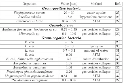
Organism Value [atm] Method Ref.

Gram-positive bacteria

Staphylococcus aureus 20 – 30 water uptake [25]

Bacillus subtilis 18.8 hypersaline treatment [26]

Enterococcus hirae 3.95 – 5.9 AFM [27]

Cyanobacteria

Anabaena flos-aquae, Nodularia sp sp. 0.79 – 1.78 gas vesicles collapse [28]

Microcystis sp. 6.4 – 10.9 gas vesicles collapse [29]

Gram-negative bacteria

E. coli 5 – 6 [25]

E. coli 5 – 10 lysozyme [30]

E. coli 0.7 – 3.1 amount of water [31]

E. coli 0.26 AFM [32]

E. coli, Salmonella typhimurium 3.5 solute distribution [33]

Ancylobacter aquaticus 1.85 gas vesicles collapse [34]

Ancylobacter aquaticus 1.06 gas vesicles collapse [35]

Pelodictyon phaeoclathratiforme 3.26 gas vesicles collapse [36]

Magnetospirillum gryphiswaldense 0.84 – 1.48 AFM [37]

[image:17.612.108.542.67.358.2]

Pseudomonas aeruginosa 0.1 – 3.95 AFM [27] Table 2.1: Comparison of the turgor pressure measured using various methods in Gram-positive, Cyanobacteria, and Gram-negative bacteria. A significant difference in measured values is observed not only when comparing different groups of organisms (e.g., Gram-positive and Gram-negative bacteria), but among the representatives of the same group as well.

(18)

the reaction to this stimulus may occur at different time scales. As mentioned above, stress on the membrane activates various osmoprotective mechanisms. Without an accurate measurement of the pressure change due to water diffusion one cannot quan-titatively study and describe the details of cell reaction to osmotic challenges. One of the possible explanations for the source of the variation in the measured turgor pressure values is that the cell is in a dynamic state, readily adapting to shifts in en-vironmental conditions or mechanical stimuli introduced by the techniques used for the measurement, which may result in turgor pressure changes occurring very fast, at the time scales shorter than the time needed for the measurement.

2.4 Stimuli and forces

E. coli

might be exposed to

(19)

Arbitrary Time

Lo

g no

. c

ells

0 3 6 9 12

[image:19.612.129.515.73.293.2]

direct count culturable count

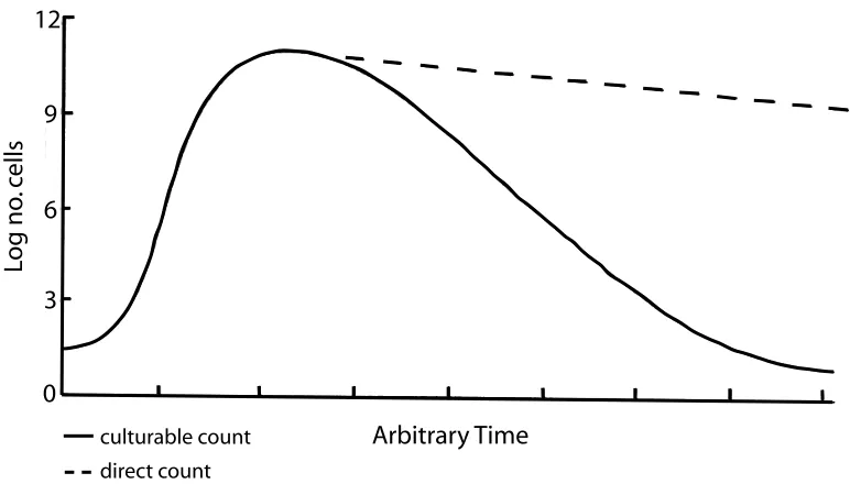
Figure 2.3: Difference in the number of bacteria estimated by the plate counting method and direct microscopy. The plate counting method introduces the bias towards organisms which can be cultured in the laboratory setting. The microscopy counts are more accurate in term of number of cells, however, they do not provide any information on their physiological state. The difference in counts from these two methods represents viable but not dividing cells [38].

(20)

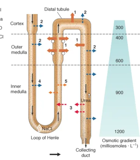
a general understanding of how it behaves and survives in its natural habitats. The habitats of E. coli can be divided into two groups: host-associated and open. How-ever, one should remember that the genomes of different forms of E. coli may vary even by 20%, which results in different phenotypes from changing patterns of gene expression [40]. This variation may be the effect of experiencing a biphasic lifestyle (host-independent and host-associated phases) and, as a consequence, exposure to various evolutionary pressures (biotic and abiotic [41]). These two environments are very different. E. coli living in the human intestine is under pressure from the biotic factors: competitors, cheaters, or host defense mechanisms. Bacteria entering the human digestive system with food are exposed to low pH when entering the stomach. In the intestine they are exposed to big variations in water content: the moisture content of feces may oscillate between 53 and 92% [42]. Bacteria in the urinary tract experience significant variations in the osmolarity, roughly 900 mOsm (Figure 2.4). Also, the composition of theE. coli population in the intestine is constantly changing with no dominant serotype [43] and may vary significantly depending on the source of the sample [44].

The challenges in the open environment are very different: temperature, UV ra-diation, low concentration of nutrients, and fluctuating osmolarity and water level. Survival depends on how well E. coli can cope with rapidly changing conditions and adapt to them. The most important factor is water availability. Without proper water activity, cells desiccate very quickly (15 – 60 hours) [45]. If there is enough moisture,E. coli can survive many days in the environment: in sea water [41, 46, 47], fresh water [47], as well as the beach sand [48].

2.4.1 Osmosis

(21)

mea-Figure 2.4: The osmolarity changes which bacteria may be exposed to when living in the urinary tract. The content of the urine changes significantly due to resorption of valuable molecules (e.g., proteins and sugars). Active transport of NaCl and diffusion of urea, water, and NaCl increase urine osmolarity from 300 to 1200 mOsm. Figure adapted from [50].

surements were carried out between 1826 and 1846 by Ren´e Joachim Henri Dutrochet (who was the first to use terms “endosmosis” and “exosmosis” [51], Figure 2.5A) and Karl Vierordt [52]. They concluded that the rate of osmosis depends on both the nature of the salt and the concentration of the solution. Later, it was shown that also the type of membrane separating the two solutions plays an important role. This fact was subsequently used by Thomas Graham for the separation of different substances by dialysis [53] (Figure 2.5B). In 1864, Moritz Traube obtained a precip-itation membrane permeable to water (tannic acid and non-setting glue) forming a coating on a drop and, thus, initiating studies of the “endosmotic force” [54]. Jacobus Henricus van’t Hoff called the membrane which is permeable only to the solvent a semi-permeable membrane (there is no membrane that is completely impermeable to the solute) [55].

[image:21.612.257.487.66.329.2]

(22)

A B

[image:22.612.165.487.57.411.2]

C

Figure 2.5: Examples of osmometers. (A) Osmometer used by Dutrochet [56]. This type of an osmometer was used for the first quantitative measurements of osmosis; (B) Osmometer used by Graham [53]. After the discovery that the type of the membrane separating two solutions plays an important role, this type of osmometer was used by Graham to study the separation of various substances by dialysis ; (C) Osmometer used by Pfeffer [57]. Formation of a membrane in the wall of porous earthenware pots significantly increases the range of values which can be measured in this type of the osmometer.

(23)

with that of a gas, van’t Hoff deduced thatthe osmotic pressure of a solution is equal to the pressure which the dissolved substance would exercise in the gaseous state if it occupied a volume equal to the volume of the solution [58]. The first direct determi-nation of osmotic pressure was carried out by Wilhelm Pfeffer and later perfected by Harmon Northrop Morse [59].

2.4.2 Adaptation to increasing osmotic pressure

E. coli cells can grow in a variety of environments, from very aqueous to those with high salt concentration. The bacterial growth in environments with such a wide range of osmolarities is a great challenge for cell physiology. A very high membrane per-meability for water compared to other molecular species (perper-meability coefficient for water: 10−6 to 10−2 cm/s depending on the cell type; permeability coefficient for Na+: 10−12 cm/s [60, 61]) makesE. coli sensitive to osmolarity changes in the environment. In case of an increase in osmolarity the cell has to retain water necessary for growth and biochemical reactions by, e.g., increasing the osmolarity of the cytoplasm. At the same time, the solutes accumulated in the cytoplasm (by transport or synthe-sis) to reduce these osmotically induced changes can’t destabilize the homeostasis of the cell or cause a disruption of biochemical processes (this is why they are called compatible solutes). Such solutes include K+_{, amino acids (glutamate, proline) and}

their derivatives (peptides), quaternary amines (glycine betaine, carnitine), sugars (sucrose, trehalose), and tetrahydropyrimidines (ectoines) [62].

(24)

maximum uptake rate being 10pmol/cm2_{s) [63, 64]. Simultaneously, to balance the}

electric charge of accumulated K+, cells synthesize glutamate. A 0.5 M NaCl upshock induces an increase of glutamate concentration to 300 nmol/mg dry mass within 10 minutes [65].

In the next phase, to avoid very high internal ionic strength, E. coli substitutes potassium and glutamate with zwitterionic (a molecule with a positive and a negative electrical charge) or neutral solutes (neutral and zwitterionic solutes are more favor-able to protein stability). A 0.5 M NaCl upshock induced synthesis of the disaccharide trehalose to a concentration of 300 nmol/mg dry mass within 2 hours [65]. The sec-ond phase response may be much faster if the compatible solutes are present in the medium. The most common zwitterions are glycine betaine and proline [21, 62, 66]. These compounds can be accumulated in the periplasm at a high concentration. For example, uptake of glycine betaine through a high affinity betaine transport proU of more than 1 µ mol/mg of dry mass translates to cytoplasmic concentration of close to 1 M [65, 67]. Glycine betaine can also improve a diminished growth rate due to the presence of high salt concentration [67].

2.4.3 Reaction to decrease in osmotic pressure

Bacteria are very often exposed to sudden changes in osmolarity of the surrounding fluids. Membranes are most permeable to water (permeability coefficient varies from 10−6 to 10−2 cm/s depending on the cell type [60, 61]) and least permeable to charged molecules like ions (permeability coefficient for Na+ is 10−12 cm/s [60]). However, membrane permeability (measure of the ability of a membrane to allow molecules to pass through it) is not high enough to release tension from the membrane fast enough and prevent it from rupturing.

(25)

are due to their leakage through the hole in the cell wall and membrane produced by the tension.

The discovery of MS channels, especially MscL (Mechanosensitive channel of Large conductance), made them a perfect candidate to explain this phenomenon. The size and types of the molecules which might be released through these channels was stud-ied using various methods (Table 2.2), however, some controversy concerning the size and the mechanism of release still remains. Schleyer et al. [70] looked at the amino acids that E. coli releases during osmotic shock. Surprisingly, aspartate and gluta-mate were released whereas alanine, lysine, and arginine were not. Ajouz et al. [65] have shown that thioredoxin (11.5 kDa), and Berrier et al. [71] have shown that the heat shock protein DnaK (41 kDa) and elongation factor Tu (52 kDa) are released during osmotic shock through MscL channels. However, the work by van den Bo-gaart et al. [72] contradicted these results. They have shown that MscL can release proteins up to at least 6.5 kDa, but not bigger. In their experiments, liposomes (artificially-prepared lipid vesicles) with MscL reconstituted were monitored for the release of fluorescently labeled species upon channel activation. Molecules with a mass bigger than 6.5 kDa, i.e., thioredoxin (11.5 kDa), histidine-containing protein HPr (9 kDa), and α−lactalbumin (14 kDa), all labeled with Alexa fluor 633 (∼ 1 kDa), were not released from the liposomes upon MscL gating. Using the crystal structure of thioredoxin, histidine-containing protein HPr, and α−lactalbumin, the sizes of these molecules (25 x 30 x 35 ˚A, 32 x 32 x 33 ˚A, and 52 x 32 x 34 ˚A, respec-tively) are comparable to or bigger than the estimated size of the MscL pore. Based on channel conductance and the fact that poly-L-lysines with a diameter bigger than 37 ˚A blocked the conductance of the channel, the size of the MscL pore is estimated to be 26-46 ˚A [73, 74].

(26)

Molecule Mass Amount Shock Method Ref.

potassium 39 Da 60% 1000 mOsm flame photometer [63]

potassium 39 Da 85% 0.2 M NaCl valinomycin electr. [76]

potassium 39 Da 85% 0.25 M NaCl flame photomety [70]

potassium 39 Da 50-85% 0.2 M NaCl valinomycin electr. [65]

amino acids 80% 10x dilution radioactivity [77]

PO3−₄ 95 Da 100% radioactivity [77]

TMG 210 Da 80% 0.5 osm radiolabeling [78]

galactose 180 Da 40% 10x dilution radiolabeling [78]

nucleotides ∼300 Da 40% 500 mOsm UV absorption [78]

ATP 507 Da 76% 0.2 M NaCl luciferin/luciferase [76]

ATP 507 Da 5% [79] [70]

lactose 342 Da 82% 0.2 M NaCl radiolabeling [76]

glutamate 145 Da 83% 0.2 M NaCl enzymatic assay [76]

glutamate 145 Da 75% 0.4 M NaCl phenol method [70]

glutamate 145 Da 80% 0.5 M NaCl enzymatic assay [65]

Rb+ _{85 Da} _93% _{0.2 M NaCl} _{radiolabeling} _[76]

trehalose 342 Da 75% 0.4 M NaCl phenol method [70]

trehalose 342 Da 70% 0.5 M NaCl phenol method [65]

aspartate 1333 Da 80% 0.4 M NaCl phenol method [70]

glycine betaine 117 Da 90% 0.5 M NaCl radiolabeling [65] thioredoxin1,2 14.8 Da 100% 0.5 M NaCl enzymatic assay [65]

DnaK1 _{41 kDa} _60% _{20% sucrose} _{immunoblotting} _[71]

DnaK1 _{41 kDa} _{immunoblotting} _[80]

RFP 862 Da 44% 20% sucrose fluorescence [80]

EF-Tu1 52 kDa 70% 20% sucrose immunoblotting [71]

p-nitrophenyl

Est551 55 kDa 89% 20% sucrose

butyrate [81]

glutathione3 _{307 Da} _35% _{fluorescence-burst} _[72]

R9C3 _{1 kDa} _50% _{fluorescence-burst} _[72]

insulin3 _{5.7 kDa} _60% _{fluorescence-burst} _[72]

BPTI3 6.5 kDa 30% fluorescence-burst [72]

protein content1 _10% _{20% sucrose} _{electrophoresis} _[75]

DsbA*1 _{23 kDa} _90% _{0.5 M sucrose} _{enzymatic assay} _[82]

DsbC*1 25 kDa 73% 0.5 M sucrose enzymatic assay [82] Table 2.2: Molecules released from E. coli cells during osmotic shock. TMG =

methyl−β−D−thiogalactoside, RFP = trimethylpyrrocorphin and sirohydrochlorin,

BPTI = bovine pancreas trypsin inhibitor, Est55 = carboxylesterase of Geobacillus

stearothermophilus, EF-Tu = elongation factor Tu, R9C = bradykinin R9C, DsbA* and

DsbC* = leaderless (signal sequence deleted). The phenol method is described in [83]. 1 =

(27)

released during osmotic shock are identical with those released during electroporation. It is known that electroporation causes formation of pores in biological membranes that can be healed [84, 85]. The similarity in protein release for these two techniques may indicate that osmotic shock also causes transient holes in the cell membrane. Molecular dynamics studies [86] have shown that at a loading rate of 660kN/(m×s) the membrane ruptures before the MscL channel gets activated. However, once the internal and external pressures are equalized, the liposome can close itself by heal-ing the rupture. There exists no experimental proof yet that this is also true for an E. coli exposed to osmotic shock, but the membrane sealing was experimentally demonstrated for red blood cells [87].

2.4.4 Examples of “real” osmotic shocks

Bacteria can be found inside and on the surface of the human body, as a part of the regular microflora or as an effect of infection. The largest population of bacteria can be found in the intestine, in the mouth, and on the skin. These bacteria have to be in osmotic equilibrium with the surrounding fluids (intracellular or extracellular). An interesting problem to consider is the osmotic pressure change which these cells are exposed to when diluted with water. As an example, the osmolarity change for bacteria inhabiting three different regions of the human body (mouth, intestine, and urinary tract) can be calculated using equation (2.1), where ∆πis the osmotic pressure change, R is the gas constant, T is the temperature, and ∆C is the concentration change.

∆π=RT∆C. (2.1)

(28)

blood, but the composition may vary significantly due to diffusion and resorption. For example, the osmolarity and the content of urine changes significantly between the beginning (where it is close to the osmolarity of other physiological fluids) and the end of a nephron (where it is mostly water, urea, and ions). Most of the water and solutes (e.g., proteins, sugar, or NaCl) that are filtered in the nephron are resorbed. Active transport and diffusion change both the composition and the osmolarity of the urine (Figure 2.4). Interestingly, the composition of saliva and sweat depends on the rate of secretion. For example, the amount of sodium in saliva increases with increas-ing rate of flow (from 20 mM at 3 mL/min to 90 mM at 40 mL/min) [39]. Assumincreas-ing that sodium is the only osmolyte in the saliva, one can estimate the osmolarity to vary between 20 and 90 mOsm. Using this value and T = 310 K (body temperature) to solve equation 2.1, one obtains an estimate of the osmotic pressure change that bacteria inhabiting our mouth are exposed to when one drinks a glass of water that varies between 0.5 and 2.3 atm.

Feces represent the sum of the indigestible parts of ingested food, digestive juices and cells shed by the mucous membrane lining of the digestive canal. In human, the total quantity of liquid passing into the gut probably amounts to 10 liters a day, of which all but about 100 ml are resorbed [39]. The typical stool osmolarity is 290-300 mOsm per kg [88], however, the moisture content of the feces may range between 53 and 92% [42]. The osmolarity of the intestinal content depends on the diet (the products of bacterial fermentation) and the amount of undigested or unabsorbed food in the intestine (which increase the osmolarity of the intestinal content causing lesser water reabsorption and smaller change in the concentration of ions [42, 89]). Taking 290-300 mOsm per kg as a typical osmolarity of the stool, the osmolarity change which the bacteria are exposed to when going into water is about 7.7 atm.

(29)

the recommended pressure of the car tire is 2 atm.

urine osmolarity osmotic viable bacteria/mL

number [mOsm/L] pressure [atm] _{before lysis} _{after lysis} _{% survival}

1 500 12.9 200 20 10

2 1126 29 11600 2600 22.4

3 1016 26.2 7000 860 12.3

4 1012 26 2300 470 20.4

5 996 25.7 15000 3200 21.3

6 1056 27.2 2148000 548000 25.5

7 980 25.2 810000 12400 1.53

8 904 23.3 2470 160 6.5

Table 2.3: Osmotic fragility of spheroplasts induced in human urine in vitro. All samples were diluted 1 : 40000 into water. The atmospheric pressure change the bacteria were exposed to was calculated using equation (2.1). The survival count measured was based on plating. Adapted from [91].

As shown by these examples, the osmotic pressure difference which bacteria can be exposed to varies a lot (5×10−4−20 atm). Despite being a single-celled organism,

E. coli can survive a wide variety of pressure changes (Table 2.3).

2.5 Family of mechanosensitive channels in

E. coli

Mechanosensitive (MS) channels were discovered in 1987 [92], resulting in the pro-posal that they may play a crucial role in sensing osmolarity through changes in turgor pressure and protecting cells from osmotic shock. This discovery led to a very active development of research in the mechanotransduction and osmoregulation field. Subsequent discoveries demonstrated that the channels are gated by a mechanical stimulus, but left the questions concerning the mechanism and physiological rele-vance of MS channel functioning unanswered, creating at the same time even more interest in the subject.

(30)

different conductances upon application of suction pressure on the giant spheroplasts of E. coli. Moreover, activity of only some of these channels could be inhibited by the addition of Gd3+ _{ions. These results suggested not only the existence of}

multi-ple types of mechanosensitive channels in E. coli, but also demonstrated that they have different properties. Another piece of evidence for the existence of different mechanosensitive channels in the cell membrane (and their physiological role) was reported by Ajouz et al. [93]. The authors were investigating the efflux of various molecules due to osmotic downshock in the wild type and mscL− strains of E. coli. The release of some species was not disturbed in the mscL− strain, which demon-strates the involvement of different channels in the rescue of the cell during an osmotic shock. Another surprising result was that the efflux of glycine betaine occurred only upon about a 200 mM change in the external NaCl concentration, which suggested the existence of different thresholds for various channels. This was soon proven to be the case using patch-lamp technique [94].

The discovery of the gene encoding the MscL protein by Sukharev et al. [95] enabled the introduction of crystallography techniques to study MS channels. The first crystallographic structure of an MscL homolog was reported in 1998 by Chang

et al. [96]. The authors identified an MscL homolog in the bacteriumM. tuberculosis

(Tb-MscL) which exhibits an overall 37% sequence identity to E. coli MscL (Eco-MscL). Tb-MscL is a homopentamer consisting of two domains, a TM domain and a cytoplasmic domain. The TM1 helix that forms the pore of the channel is one of the most highly conserved regions in the sequences of the MscL protein. To this day, crystal structures of a few MscL and MscS homologs have been solved in different conformational states [97, 98, 99].

(31)

in providing protection against osmotic shock. More recently, more genes coding pro-teins having mechanosensitive channel activity were characterized: ybdG [100], ynaI,

ybiO, and yjeP [101] reaching the total number of 7 different types of MS channels inE. coli (Table 2.4).

Gene Year of characterization Reference

mscL 1994 [95]

yggB 1999 [22]

kefA 1999, 2002 [22, 102]

ybdG 2010 [100]

ynaI 2012 [101]

ybiO 2012 [101]

yjeP 2012 [101]

Table 2.4: Genes coding the activity of all seven mechanosensitive channels in E. coli. The

first gene coding MS channel activity (mscL) was identified seven years after the discovery of

MS channels. The last three mechanosensitive genes (ynaI,ybiO, andyjeP) were identified

25 years after the discovery of MS channels.

2.6 Standard ways of studying MS channels in

bac-teria

2.6.1 Theoretical modeling

One of the methods used to study mechanosensitive channels is theoretical modeling, predicting the reaction of the channel (gating probability) to a given perturbation.

A single channel is modeled as a two-state protein. It can be in a closed state, characterized by the energy Eclosed, or in an open state, characterized by the energy

Eopen. The equilibrium between these two states depends on the value of the external

(32)

STATE WEIGHT

e–βE_closed

e–β(E_open–τ∆A)

closed

open

Figure 2.6: Mechanosensitive channel modeled as a two-state protein. The closed state

has energy Eclosed and the open state is characterized by energy Eopen. The external force

is pictured as a loading device attached to the channel. The lowering of the loading device

(open state) stabilizes the open state by descreasing its energy value by τ∆A. Figure

adapted from [60].

0 2 4 6 8 10

-5 -2.5 0 5 7.5

2.5 10

E(R)

R

closed open Increasing_driving

force

Figure 2.7: Energy landscape of the two-state channel as a function of its radius. The curves correspond to different values of the externally applied force (tension). Depending on its value, the balance between open and closed state can be shifted. For small values of tension the closed state is energetically favorable (first curve). As the tension increases, the open state decreases its energy and the balance shifts towards this state being more stable (last curve). Figure adapted from [60].

(33)

Using this theoretical model we can quantitatively predict the state of the channel by calculating its gating probability. To do so, one can use the Boltzmann distribu-tion, which states that finding the a state with a given energy E is

p(E) = e

−βE

Z , (2.2)

whereZ is called the partition function and is a sum of all possible states (it is a nor-malization constant determined by the requirement that the sum of all probabilities is equal to 1). We can calculate the probability of the channel being in an open state as a function of applied tension τ as

popen =

e−β(Eopen−τ∆A)

e−β(Eopen−τ∆A)+e−βEclosed =

1

1 +e−β(τ∆A−Egate), (2.3) where Egate=Eclosed−Eopen is the gating energy.

As already mentioned, the tension in the membrane is the external stimulus that changes the state (closed or open) of the protein. However, the protein may also influence the energy of the membrane [103]. The conformation of the protein depends on the tension value applied through the bilayer; however, the opening of the channel causes deformation of the surrounding lipid membrane. One can thus model the free energy of the protein-membrane system as the sum of energies associated with the state (conformation) of the protein and energies associated with the deformation of the membrane. Surprisingly, the values of these energies are very similar to the energy difference between the channel conformational states [104, 105]. This suggests that the mechanical properties of the lipid bilayer surrounding the protein will have a great impact on the channel gating.

(34)

required to open mechanosensitive channels.

2.6.2 Electrophysiology

The application of patch-clamp techniques to giant spheroplasts of E. coli led to the discovery of mechanosensitive channels [92]. Delcour et al. [107] were the first to re-port successful reconstitution of bacterial mechanosensitive channels into liposomes, which showed that the small size of bacteria is no longer a factor that excludes elec-trophysiology from the possible experimental techniques in this field (Figure 2.8 A). The parameters for channels characterized in spheroplasts and reconstituted in lipo-somes are very similar [95]. The same activity of a protein in its natural environment (spheroplasts with all the other proteins present and natural E. coli’s lipids) and in the artificial environment (liposomes) indicates that the gating tension is trans-mitted through the only element these two environments have in common, the lipid bilayer, and that protein-lipid interactions play a fundamental role in channel gating. The reconstitution of MscL into various lipid environments (synthetic phosphatidyl-choline (PC) containing monosaturated chains of 14, 16, 18, 20, and 22 carbons) further proved that gating of the channel is influenced by the surrounding lipids. The pressure needed to activate MscL was lower in the PC16 (phosphatidylcholine with chains of 16 carbons) environment when compared to the PC20 (phosphatidylcholine with chains of 20 carbons) environment (Figure 2.8 B). Interestingly, the shape of the pressure dependence curve remains the same, with the curve being shifted by some value [108]. Based on the experimental data the authors concluded that the two physical mechanisms influencing MS channel gating are hydrophobic mismatch between the protein and the lipid environment (which can be controlled by reconsti-tution into lipid vesicles with different acyl chain lengths) and the bilayer curvature (which can be modified by unsymmetrical addition of, e.g., lysophosphatidylcholine (LPC)) [108].

(35)

A

B

C

Figure 2.8: Characterization of mechanosensitive channels inE. coli by the electropysiolog-ical measurement. (A) The current traces of MscS and MscL reconstituted into liposomes. The images beneath the trace show the geometry of the patch for a given value of the applied pressure. The data obtained by simultaneous measurement of the current and a function of applied pressure (electrophysiology) and observation of patch geometry (confo-cal microscopy) allows one to (confo-calculate the tension (equation 2.4) and correlate this value with the number of observed MS channel activities: (a) resting state, (b) opening of the first MscS channel, (c) midpoint activation of MscS, (d) saturation of MscS activity, (e) opening of the first MscL channel, (f) midpoint activation of MscL, (g) saturation of MscL activity,

and (h) rupture of the patch. Scale bar is 1 µm. Adapted from [110]. (B) Probability

(36)

technique and simultaneous imaging of the curvature of the patch, allowed us to conclude that the parameter regulating the MscL gating is tension, not pressure [74, 108, 109] (Figure 2.8 C). The image of the patch enables a measurement of its radius (R) for a given value of the applied pressure (p). Knowing this relationship, one can calculate the tension (τ) using Laplace’s law

τ = pR

2 . (2.4)

The existence of various conductances inE. coli membranes was reported [76, 94], suggesting the existence of various types of MS channels. However, only the identi-fication of the genes coding proteins with MS channels activity allowed the detailed characterization of individual channels (Table 2.5). Until 2012 it was believed that there is a hierarchy in the opening of MS channels, meaning that the tension required to open a given channel is correlated with its conductance. The experimental results indicated that the first channel to open was the one showing MscM activity, and, as the tension increases, MscS and MscK would gate before the MscL opening, which gates near the membrane rupture threshold [111]. However, the characterization of YjeP, YnaI, and YbiO channels proved that this rule is no longer valid (Figure 2.9). YjeP gates at a tension close to that needed to activate MscS or MscK, but it has a much lower conductance. YnaI and YbiO gate at the tension near the one needed to activate MscL, but their conductances are 100 pS, 900 pS, and 3000 pS, respectively [101]. Interestingly, the electrophysiological activity of YbdG can’t be observed unless the mutation in β domain is introduced (V229A) [101].

(37)

Channel Size [aa] PL:PX Current amplitude [pA] Conductance [pS]

MscL 136 1 90 3000

MscS 286 1.6 25 1250

MscK 1120 1.85 17.5 875

YbdG 415 – 7.5 300 (*)

YnaI 343 1.05 2 100

YbiO 741 1.21 17 900

YjeP 1107 1.64 5-8 350

Table 2.5: Characterization of mechanosensitive channels in E. coli using electrophysio-logical techniques. The size of the protein does not correlate well with its conductance or

gating tension measured with respect to the MscL activation tension (PL : PX). There

is also lack of correlation between the gating tension and the conductance of the channel, suggesting that the increase in tension value does not guarantee opening of the channels

which allow a bigger flux of material through a single channel. (*) the mutation in the β

domain (V229A) in necessary for electrophysiological activity of YbdG. Table constructed based on [101].

Figure 2.9: Comparison of the relative pressure needed to activate various MS channels.

The values for MscS homologs (PX) are reported with respect to the activation pressure of

MscL (PL : PX). Values larger than 1 mean that the tension needed to activate a given

channel is lower than the tension needed to activate MscL channel. Figure adapted from [101].

(38)

influ-ences the gating of both MscL and MscS [110] and the presence of ethyl or propyl parabens causes their spontaneous activation (the effect is reversible) [113]. Recent studies show that MscL can be engineered to show light-gated activity through the modification of the protein (G22C mutant and a cysteine-reactive spiropyran photo-switch) [114] or through reconstitution into a lipid vesicle containing a light-sensitive lipid mimic undergoing trans-cis isomerization [115].

2.6.3 Plating assay

Protection against osmotic shock as a function of mechanosensitive channels in cell physiology was postulated at the time these channels were discovered [92], and the assay testing this assumption was published only 12 years later [22].

To test the role of a given channel (or the lack of such) in cell physiology downshock assay is used (also known as survival assay or plating assay). A single colony is inoculated into 5 ml of LB and grown overnight. Next morning, the culture is diluted into 20 ml of fresh LB to a final OD600 of 0.05. Once the culture reaches an OD600

of 0.3, it is diluted 1:10 into LB supplemented with 0.5 M NaCl and grown again to OD600 ∼ 0.3. The culture is then diluted 1:20 into LB (shock) and LB supplemented

with 0.5 M NaCl (control) and incubated for 10 min at 37◦C. After the incubation serial dilutions are made into the medium of the same osmolarity (0 M NaCl for the shock sample and 0.5 M NaCl for the control). A small aliquot of each serial dilution (5 µl) is spotted on an agar plate of matched osmolarity (0 M NaCl for the shock sample and 0.5 M NaCl for the control). Plates are incubated overnight and the next day the survival rate is calculated based on the number of colonies for a shock sample normalized to a number of colonies for the control sample (Figure 2.10).

(39)

0 M NaCl shock 0.5 M NaCl shock

mscL

pmscSmscK

mscS

A

[image:39.612.233.419.77.345.2]

B

Figure 2.10: Survival of mechanosensitive channel mutants after exposure to osmotic shock. (A) Agar plates showing growth of colonies after overnight incubation for the shock sample (0.5 M NaCl shock) and the control sample (0 M NaCl shock). Rows represent aliquots of the same dilution, columns represent serial dilutions. (B) Survival rate for strains expressing MscL, MscS, and/or MscK from the chromosome, and/or from the plasmid (pmscS) after exposure to a 0.5 M NaCl shock. The survival rate is calculated based on the number of colonies of cells exposed to osmotic challenge which grew after the recovery period, normalized by the number of colonies for control samples (not exposed to osmotic challenge). Adapted from [22].

cell. This may not be the case if two or more cells formed a minicluster, resulting in a single colony after an overnight incubation. Another source of error when calcu-lating the survival rate is the normalization factor. The control sample is grown on a high salt plate, which may limit growth of some percentage of the cells. Also, the normalization by OD600 of a given sample when it was exposed to osmotic shock may

introduce a systematical error. The same OD600 does not always correspond to the

same number of cells for a given strain [116], so this parameter should be controlled for (for the modified plating assay protocol with comments see Appendix A).

(40)

how-ever, they did not gain as much interest as the assay described above.

Type of assay Reference

colony count [22]

amount of A260 absorbing material released [22]

Live/Dead BacLight dyes and plate reader [117] microscopy and staining [118] flow cytometry and staining [118] amount of released DNA (fluorescence) [119] light scattering with a stopped-flow device [120]

Table 2.6: Various techniques used to calculate the number of cells surviving an osmotic shock. The colony count method is the most popular one. The readout of this method is cellular growth. The other methods are based on the amount of released material (measured by absorbance or fluorescence) or the integrity of cell envelope (staining methods).

2.7 Unanswered questions - motivation for further

studies

2.7.1 How many channels are there in a cell?

(41)

of the cell to a given osmotic stimulus will vary. If this number is constant, the cells in the population should respond differently depending on their size. As shown by numerous biophysical models, both the number of such channels and their variability can impact many physiological processes, including osmoprotection, channel gating probability, and channel clustering. [121].

2.7.2 What is the role of MS channels in cell physiology?

From the very first moment MS channels in bacteria were discovered, their impor-tance in osmoregulation was postulated [92], and only a few years later a proof of their function as defense mechanisms against the osmotic shock was experimentally affirmed [22]. It is known that wild-type cells express seven types of mechanosensitive proteins [101] and the reason for this variety should be explained by studying their response to the same perturbation. Bulk osmotic shock experiments revealed that the presence of MscL or MscS [22], or an overexpression of one of the MscS homologs (in the absence of other mechanosensitive channels), can rescue the cell from a hypoos-motic shock [100, 101]. This fact indicates that all of the channels have a potential to rescue the cell from a very severe osmotic downshock, and, theoretically, the presence of all of them is not crucial.

The identification of genes coding all mechanosensitive channels in E. coli (Table 2.4) opens the possibility of creating a strain carrying any desired combination of MS channels. The comparison of the physiological behavior or response to osmotic shock for various mutants makes it possible to study the physiological relevance of variouis MS channels, their response to the same perturbation, time scale of this response, their sensitivity, and potential interactions.

2.7.3 What is the role of single-cell stochasticity?

(42)

even if cells are genetically identical [122]. There are many possible explanations for the phenotypic heterogeneity of an isogenic population: various “ages” of the cells, the cell cycle stage (fluctuations in the transcriptional activity), different volume or density of cells in a population, or, finally, intrinsic (stochastic effects in transcription, translation, or replication) and extrinsic (fluctuations in the number of polymerases or ribosomes) noise in gene expression. Whatever the source of such variation is, it may result in a differential sensitivity to stress among the members of a given popu-lation.

The role of this single-cell stochasticity is unclear. One of the explanations for the diverse patterns of gene expression resulting in phenotypic subpopulations is fitness advantage. The conditions in the natural environment tend to fluctuate, so if the distribution of phenotypes is broad, the chances that one of the subpopulations will remain viable increase. Such a scenario means that bacteria are able to anticipate and adjust to sudden changes in the environment. Another possibility is that cells may vary not only in the gene expression profile but also other physiological parameters, e.g., the growth rate. This suggests that members of the same population may react to changes in the environment at different time scales. One subpopulation may be able to respond to a very fast change, whereas the other subpopulation may respond only to persistent and slow change in the environment.

(43)

Chapter 3 Single-cell response to medium

exchange

3.1 The mystery of seven channels

Mechanosensation is a ubiquitous phenomenon found across all domains of life. In bacteria, one of the manifestations of such processes is in the context of osmopro-tection, where it has been proposed that the presence of MS channels in the cell membrane allows these cells to survive an osmotic shock. These channels gate in response to an increase in membrane tension and prevent membrane rupture by me-diating a net efflux of water and small molecules. The first bacterial mechanosensitive channels were discovered in 1987 [92] and in the intervening period a whole battery of such channels has been discovered with seven different mechanosensitive channels now demonstrated experimentally inE. coli [101]. These channels have been characterized with electrophysiological measurements (Table 2.5). Interestingly, the characteriza-tion of YjeP, YnaI, and YbiO violates the hierarchy rule for opening MS channels, which hypothesizes that the tension required to open a given channel correlates with its conductance. One of the puzzles left unresolved in the wake of the discovery of this mechanosensitive protein diversity is why there are so many distinct mechanosensi-tive channels in E. coli and what their significance for cell physiology is. The work presented here partially addresses these questions.

(44)

Specifically, until now the survival of cells subjected to osmotic shock has been mainly characterized in bulk assays, in which a large population of cells is shocked and the resulting survival fraction is measured through colony counting. The comparison of the survival rate for various deletion mutants has made it possible to study the contribution of a particular channel to cell survival after exposure to a 0.5 M NaCl shock. Based on these studies, the presence of MscL or MscS is believed to provide osmoprotection at near wild-type level [22].

These assays, although very informative, reflect the population response to a large amplitude (0.5 M NaCl) and not well-controlled rate of change in the medium osmolar-ity (about 1 s). These conditions may seem extreme when compared to the osmolarosmolar-ity changes which E. coli may be exposed to in its natural habitat. For example, the osmotic challenge due to rainfall will be different for E. coli in the shallow marine water when compared to one in an open ocean. In addition, some of the channel properties may be too subtle to be discovered by means of this assay. For example, the inactivation of MscS channels in the patch clamp measurement can be observed only when the pressure is applied gradually [120].

(45)

3.2 Single-cell observation

The physiology of MS channels has been studied extensively over last twenty years. However, until now the survival of cells subjected to an osmotic shock has mainly been characterized in bulk assays, in which a large population of cells is shocked and the resulting survival fraction is measured through colony counting [22]. The measurement of the mean response of the cell population makes this assay blind to many parameters, e.g., variety of responses among cells from a given population, or the time and mechanism of cell envelope rupture. In addition, the kinetics of the addition of a shock medium is not well-controlled, which may result in observing only one (out of many possible) types of cell responses.

In this work, we present a single-cell method for measuring cell survival after an osmotic challenge and the influence of the kinetics of the osmotic treatment on the survival of various MS channel deletion mutants. This method allows us to control the medium exchange rate and perform a quantitative measurement of the osmolarity gradient based on fluorescence signal change. The observation of single cells as a function of the recovery time after an osmotic challenge allows for an accurate determination of the fate of individual cells (death or division), as well as the time interval between the osmotic challenge occurrence and cell death.

(46)

Chamber

0.5 M NaCl

0 M NaCl Negative pressure

pump

Flow

Valve

Figure 3.1: A schematic picture of the experimental setup used for the single-cell

observa-tion of E. coli mutants exposed to a well-controlled osmotic challenge. The inputs of the

flow cell are connected to reservoirs with high (0.5 M NaCl) and low (0 M NaCl) osmolarity media. The osmolarity of the medium in the viewing chamber is controlled by the valve. The constant flow of medium through the experimental system is guaranteed by the con-nection to the syringe pump through the output of the flow cell. The details of the assembly method are described in Appendix B.

in the chamber. Next, the real time medium exchange calibration was recorded for one of the positions.

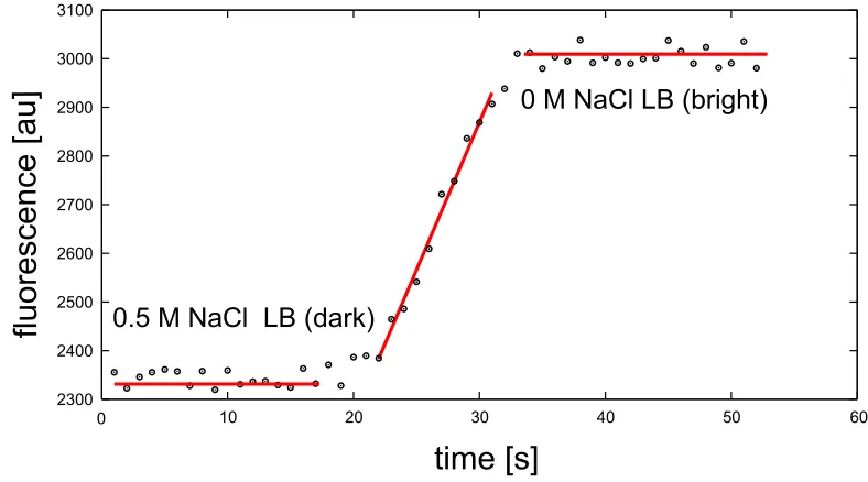
In order to monitor the rate of the medium exchange, both high and low salt media were supplemented with 250 nM calcium-sensitive Rhod-2 dye. The shock medium (0 M NaCl LB) was also supplemented with 100 µM CaCl2 to create a difference

in the fluorescence signal between these two media. The fluorescence signal of the medium in the flow cell was recorded in real time during cell exposure to osmotic challenge. The rate of medium exchange was measured based on the signal intensity change as the high salt medium (low signal) was substituted by the low salt medium (high signal). The quantitative measurement of the rate exchange was performed by curve fitting to the recorded signal (f luo) (Figure 3.2). The minimum (0.5 M NaCl medium) and the maximum (0 M NaCl medium) signal level was calculated as the average value (f luomin and f luomax, respectively). The standard deviation for both means was calculated as well (∆f luomin and ∆f luomax, respectively). The difference

between these two values was taken as the fluorescence signal change corresponding to a 0.5 M NaCl osmolarity drop (f luomax-f luomin). Next, a linear fit was performed

(47)

0 10 20 30 40 50 60 2300 2400 2500 2600 2700 2800 2900 3000 3100

time [s]

fluorescence [au]

0.5 M NaCl LB (dark)

[image:47.612.124.518.80.299.2]

0 M NaCl LB (bright)

Figure 3.2: Fluorescence signal of the medium as a function of time during the medium exchange in a flow chamber. The medium is changed from 0.5 M NaCl LB with 250 nM calcium-sensitive 2 dye (dark) to 0 M NaCl LB with 250 nM calcium-sensitive

Rhod-2 dye and 100 µM CaCl2 (bright). The rate is calculated by fitting a straight line to

three regions: minimal fluorescence level, maximal fluorescence level and the middle of the calibration curve. The error analysis is discussed in the text.

in arbitrary units (called here counts),timeis measured in seconds, andais measured in counts per second. The uncertainties in determining the slope (a) and the intercept (b) of the fitted curve were obtained from the fitting as well (∆aand ∆b, respectively). The correlation coefficient R2 _{was kept higher than 0.95 (if the correlation coefficient}

of the linear fit was lower than 0.95, the fit was performed to only a part of the middle of the trace). The rate (R) was calculated by dividing the slope of the fitted curve (a) by the value of the recorded signal (f luo). The uncertainty in the rate determination (∆R) was calculated by error propagation:

∆X

X =

s

∂f

∂A ×∆A 2

+

∂f

∂B ×∆B 2

, (3.1)

(48)

function this calculation resulted in the following equation:

∆R

R =

s

a×∆f luomax

(f luomax−f luomin) 2

2

+

a×∆f luomin

(f luomax−f luomin) 2

2

+

∆a

f luomax−f luomin

2

.

(3.2) After the calibration, the shock medium (0 M NaCl LB) was substituted with a medium of the same osmolarity, but without the dye and CaCl2. The recovery of

cells was recorded by taking snapshots at previously chosen positions, one snapshot per minute during a two to three hour period. In order to supply enough nutrients and oxygen to the recovering cells, the 0 M NaCl LB medium was pumped through the chamber during the recovery phase at a constant speed of 10 µl/min.

The survival rate and the fate of each individual cell was determined based on the data collected during the recovery phase. A cell was counted as a survivor based on its division (Figure 3.3, cells marked with an arrow). The rest of the cells were classified as dead (Figure 3.3, cells marked with a star) or intact, non-dividing cells (Figure 3.3, cells marked with a triangle). The dead cells were further divided into subclasses (described later). The percentage of the population which survived the shock was calculated as the ratio of the number of dividing cells to the total number of cells from twenty fields of view. The error in the calculated survival rate was taken as the fraction of intact, non-dividing cells with respect to the total number of cells.

3.3 Rate dependence

(49)

mechanosensi-0 min 40 min 60 min

* *

[image:49.612.112.539.301.515.2]

*

Figure 3.3: Image sequence showing the recovery of MJF465 cells exposed to a 0.5 M NaCl

shock at 100 µL/min. Cells can be classified into 3 groups: cells that survived the shock

and divide (marked with an arrow), cells which are intact, but do not divide (marked with a triangle), and cells that died as a result of the osmotic challenge (marked with a star). As discussed in the text, the dead cells can be further classified based on their morphology.

0 20 40 60 80 100

0 0.2 0.4 0.6 0.8 1 1.2 1.4

medium exchange rate [1/s]

Delta7 MJF465

Frag1 MJF612

MJF429

%

s

ur

vi

va

l

Figure 3.4: Survival as a function of the rate of medium exchange. Strains Frag1

(wild-type), MJF429 (∆mscS ∆mscK), MJF465 (∆mscL ∆mscS ∆mscK), MJF612 (∆mscL

∆mscS ∆mscK ∆ybdG), and MJF641 (all seven mechanosensitive channels knocked-out)

were exposed to a 0.5 M NaCl shock performed at various rates of medium exchange. The survival depends on the rate of the osmotic challenge as well as on the type of MS channels present.

(50)

Strain Frag1 (wild-type) was used as a positive control and, as expected, survives at a level close to 100% for the whole range of medium exchange rates tested (for a comparison with the previously published values, see Figure 2.10 and Table 3.1). Strains MJF429 (∆mscS ∆mscK), MJF465 (∆mscL∆mscS ∆mscK), and MJF612 (∆mscL ∆mscS ∆mscK ∆ybdG) show various survival levels (0% - 90%) depend-ing on the kinetics of medium exchange. Only strain MJF641, which has all seven mechanosensitive channels deleted, did not survive a 0.5 M NaCl osmotic shock, even at the slowest shock rate tested.

Strain Osmotic shock [M NaC] Survival [%] Reference

0.5 94± 1.2 [22]

Frag1

0.25 96 ±27 [100]

MJF429 0.5 82± 2.6 [22]

0.5 7.6 ±1.2 [22]

0.3 6.5 ±1.5 [126]

MJF465

0.25 6.3 ±6.3 [100]

MJF612 0.25 3.9 ±3.6 [100]

0.3 0.5 ±0.1 [101]

0.3 0.5 ±0.3 [101]

MJF641

0.3 0.6 ±0.1 [101]

Table 3.1: Previously published survival results obtained by a standard plating assay for strains used in this study. These survival rates differ significantly from the results obtained through the single-cell assay with a controlled rate of medium exchange. The rate of osmotic challenge is not controlled in a standard plating assay.

(51)

exchange rate) at the native level of expression.

Comparing the medium exchange time (and rate) resulting in a 50% survival for a given strain illustrates the idea that various channels provide protection at different time scales (Table 3.2). The comparison between the MJF429 (∆mscS ∆mscK) and MJF465 (∆mscL ∆mscS ∆mscK) strains suggests that the presence of MscL channels protects against a 0.5 M osmolarity change occurring over less than 1.7 s (50% survival for medium exchange over 2.5 s for strain MJF465 versus less than 1.7 s for strain MJF429), whereas YbdG provides enough protection to guarantee a 50% survival after a 0.5 M osmolarity change occurring over 2.5 s (50% survival for medium exchange over 5.8 s for strain MJF612 (∆mscL∆mscS ∆mscK ∆ybdG) versus 2.5 s for strain MJF465). Channels YbiO, YjeP, and YnaI acting together may be sufficient for protection against a 0.5 M osmolarity change over more than 5.8 s.

Strain Time of medium exchange [s] Rate of medium exchange [1/s]

Frag1 1 1

MJF429 < 1.7 >0.6

MJF465 ∼ 2.5 ∼ 0.4

MJF612 ∼ 5.8 ∼ 0.2

MJF641 30 0.03

Table 3.2: Time and rate of medium exchange at which all tested strains show 50% survival. The survival of various MS channels deletion mutants depends on the rate of osmotic challenge. This suggests that all mechanosensitive channels may contribute to cell survival. However their contribution to cell protection against osmolarity change varies depending on the rate.

3.4 Death mechanisms

(52)

as an effect of rupture of all three layers of cell envelope and release their content [22, 119] (for cartoons illustrating this assumed fate of the cell after an osmotic shock see [126] and [127]). It has only recently been proposed that the cell lysis may result in the existence of various morphological forms and the rupture of all three layers of the cell envelope does not have to occur (for the cartoon illustrating various possible scenarios see [128]).

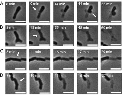
The results presented in this work are based on the observation of individual cells during and after a controlled osmolarity change. Direct observation allowed us to notice various changes in cell morphology leading to cell death (Figure 3.5).

(53)

A

B

C

D

8 min

9 min 14 min 44 min 66 min

[image:53.612.122.526.70.384.2]

Figure 3.5: Image sequences showing typical cell morphology changes after exposure to osmotic challenge leading to cell death as a function of time. (A) Bleb formation, arrows indicate the region of the cell where the blebs were formed; (B) Morphological change interpreted as a membrane rupture without formation of a bleb. The arrow indicates the location of a potential rupture; (C) Cell releasing its content (“fading”) without a clear sign of envelope damage. Arrow indicates the cell of interest; (D) Bursting cell. The content of the cell gets suddenly released. Arrow indicates the cell of interest.)

Interestingly, the abundance of a given type of change in cell morphology due to the osmotic challenge does not seem to be correlated with the rate of osmotic exchange (Figure 3.6). For all three strains tested (MJF465, MJF612, and MJG641) the percentage of a given type of morphological change was rather constant in most of the cases. In all cases cells forming blebs were the most abundant and the cells showing signs of potential membrane rupture were least abundant. This lack of correlation with the rate of the medium osmotic shock suggests that there might be a few mechanisms involved in the formation of these phenotypes.

(54)

0 20 40 60 80

0.01 0.33 0.40 0.60 0.56 0.95 MJF465 0 20 40 60 80

0.04 0.17 0.22 0.28 MJF612 0 20 40 60 80

0.03 0.06 0.42 0.65 MJF641 bleb rupture fading exploders % d ea d ce lls % d ea d ce lls % d ea d ce lls

rate [1/s] rate [1/s]

[image:54.612.115.527.68.327.2]

rate [1/s]

Figure 3.6: The percentage of cells showing a given morphology change as a function of

the rate of medium exchange for three strains: strain MJF465 (∆mscL ∆mscS ∆mscK),

MJF612 (∆mscL∆mscS ∆mscK ∆ybdG), and MJF641 (all seven mechanosensitive

chan-nels deleted). In all cases the death mechanism is not correlated with the rate of the

osmotic challenge and the most common morphological change leading to cell death is bleb formation.

(55)

0 10 20 30 40 50 60 70 80 90 100 110 120 130 140 0 5 10 15 20 25 30

0 10 20 30 40 50 60 70 80 90 100 110 120 130 140 0 10 20 30 40 50 60 70

0 10 20 30 40 50 60 70 80 90 100 110 120 130 140 0 5 10 15 20 25 30 35

0 10 20 30 40 50 60 70 80 90 100 110 120 130 140 0 0.5 1 1.5 2 2.5 3 3.5 4 4.5 5

time [minutes] time [minutes]

abundance

rate 1/s

A=37.5 exp(-0.12 t) rate 0.62/sA=122 exp(-0.09 t)

rate 0.35/s

A=66 exp(-0.06 t) rate 0.0125/s

A

D C

[image:55.612.116.531.63.382.2]

B

Figure 3.7: Histograms showing the “time of death” of blebbing MJF465 cells exposed to

0.5 M NaCl osmotic challenge performed at various rates: 1 s−1 (A), 0.62 s−1 (B), 0.35 s−1

(C), and 0.0125 s−1 (D). The exponential decay function (Y =Aexp(−Bt)) was fitted to

the histograms (the first bin was neglected for fitting). Only the last histogram does not have a fit due to the small number of bins. The fitting parameters are listed in Table 3.3 and discussed in the text.

(56)

analysis, these cells are treated as if they died at t= 0, even though they were dead earlier. That is why, to avoid the error due to an inaccurate death time assignment for these cells, we decided to neglect the first bin.

The fitting of an exponential decay function (abundance = Aexp(−B×time)) to our histograms gave us the fitting parameters A and B, which then allowed us to calculate the time needed for a 1/e drop:

e(−Bt2)₌ 1 e ×e

(−Bt1) ₌_e(−Bt1−1)

e(−Bt2+Bt1+1) _{= 1}_, _(3.3)

where ∆t = t2 - t1 is the time after which the abundance drops by a factor of 1/e.

Equation 3.3 is correct only if

−Bt2+Bt1+ 1 = 0, (3.4)

which gives us

t2−t1 = ∆t =

1

B. (3.5)

The values of the fitting parameters and the times after which one observes a 1/e

Single Cell Analysis of the Physiology of Mechanosensation in Bacteria

of Mechanosensation in Bacteria

Maja Bialecka-Fornal

Acknowledgements

Abstract

Contents

Chapter 1

Introduction

A

B

C

1.1

Mechanosensation and mechanotransduction

1.2

Evolution of sensors and membrane channels

Chapter 2

Mechanosensation in

Escherichia

coli

2.1

Escherichia coli

as a model organism

2.2

Bacterial anatomy

A

B

2.3

Turgor pressure measurement in

E. coli

2.4

Stimuli and forces

E. coli

might be exposed to

2.4.1

Osmosis

2.4.2

Adaptation to increasing osmotic pressure

2.4.3

Reaction to decrease in osmotic pressure

2.4.4

Examples of “real” osmotic shocks

2.5

Family of mechanosensitive channels in

E. coli

2.6

Standard ways of studying MS channels in

bac-teria

2.6.1

Theoretical modeling

2.6.2

Electrophysiology

A

B

C

2.6.3

Plating assay

2.7

Unanswered questions - motivation for further

studies

2.7.1

How many channels are there in a cell?

2.7.2

What is the role of MS channels in cell physiology?

2.7.3

What is the role of single-cell stochasticity?

Chapter 3

Single-cell response to medium

exchange

3.1

The mystery of seven channels

3.2

Single-cell observation

time [s]

fluorescence [au]

3.3

Rate dependence

3.4

Death mechanisms

A

B