Multi-objective optimisation using learning automata and its applications in power systems

(1)

Multi-objective Optimisation using Learning Automata and its

Applications in Power Systems

Thesis submitted in accordance with the requirements of the University of Liverpool

for the degree of Doctor of Philosophy

in

Electrical Engineering and Electronics

by

Huilian Liao, B.Sc.(Eng.), M.Sc.(Eng.)

(2)

Multi-objective Optimisation using Learning Automata and its Applications in Power Systems

by

Huilian Liao

(3)

I would like to give my heartfelt thanks to my supervisor, Professor Q. H. Wu,

whose encouragement, guidance and support enabled me to develop a deep

under-standing of my work. Without his consistent and illuminating instruction, my

re-search work and my life could not proceed to this stage. The rere-search skill, writing

skill and presenting skill he taught me will benefit me throughout my life, as well as

his inspiring insight into life philosophy and poetry.

I would like to show my gratitude to Dr. L. Jiang, my second supervisor, for

his kind guidance with his knowledge of power systems. I would also like to thank

Overseas Research Students Awards Scheme for the financial support it provided

for my research work at the University of Liverpool.

I offer my regards and blessings to all of the members of the Intelligence

En-gineering and Industrial Automation Research Group, the University of Liverpool,

especially to Dr. W.H. Tang, Dr. M.S. Li, Dr. D.Y. Shi, Dr. T.Y. Ji, Dr. J. Buse, Mr.

L. Wang, and Dr. W.J. Tang. Special thanks also go to my friends, Lesley, Louis,

Tony, Nick, and a precious couple Trevor and Ning, for their support and friendship.

My thanks also go to the Department of Electrical Engineering and Electronics at

the University of Liverpool, for providing the research facilities that made it possible

for me to carry out this research.

Last but not least, my thanks go to my beloved family for their loving

consider-ations and great confidence in me through these years.

(4)

Abstract

Learning automata are a major branch of machine learning designed to find the

optimal action to a learning task in a random environment. Interactions with

en-vironment and repetitive learning of a number of individual units, which are

in-dependent and structurally simple, enable the learning automata to tackle complex

learning problems. Systems built with learning automata have been successfully

em-ployed in many difficult learning situations over the years. They have also been

in-vestigated in solving optimisation problems. However, the performance of the

learn-ing automata in solvlearn-ing complex optimisation problems, such as high-dimensional

optimisation problems and multi-objective optimisation problems, has not been fully

investigated. Therefore, this thesis is devoted to exploring the potential of learning

automata in solving complex optimisation problems. In the thesis, Function

Optimi-sation by Learning Automata (FOLA) and Multi-objective OptimiOptimi-sation by

Learn-ing Automata (MOLA) have been developed for sLearn-ingle and multi-objective complex

optimisation problems respectively.

In FOLA, the search domain of a complex optimisation problem is divided into

cells and represented by cell values. Each automaton of FOLA conducts

dimen-sional search actions according to the path values which are calculated based on the

cell values situated on the searching path. During the optimisation process, cell

val-ues are continuously updated using the valval-ues of the automata states, and stored in

memory. In this way, the information obtained prior to the current state can be

col-lected and efficiently used. With these approaches, FOLA is able to undertake search

in continuous states and achieve accurate solutions efficiently. To fully analyse the

performance of FOLA, it has been tested based on twenty-two benchmark functions

[1], which represent a wide range of challenging optimisation problems. FOLA has

(5)

which have been reported to solve the same benchmark functions promisingly in

lit-erature. The experimental results have demonstrated the superiority of FOLA over

the other EAs for most benchmark functions, in terms of the convergence rate and

accuracy of finding optimal solutions. FOLA has shown its capability to solve

high-dimensional multi-modal problems. The experiment also shows that FOLA is able

to greatly reduce computation time, especially for high-dimensional functions.

Most optimisation problems existing in the real world have more than one

objec-tive. These problems aim to find evenly distributed Pareto fronts which are the plots

of the objective function values of the optimal solutions [2]. They can be tackled

by combining the multiple objectives into one single objective function that can be

solved by a single-objective optimisation algorithm. However, this method suffers

from the drawback of large computation load, and has difficulty in finding

non-convex Pareto fronts. Therefore, it is important to develop alternative optimisers

that can be used for complex multi-objective problems. Based on FOLA, MOLA is

proposed to solve complex multi-objective optimisation problems. MOLA mainly

comprises two processes: the process of searching and the process of learning from

neighborhood. The process of searching is carried out through a tournament that is

held between Pareto global search and Pareto local search. This tournament can

lead to a better trade-off between exploitation and exploration, which is a

criti-cal factor in finding the optimal solution. In the process of learning, the

relation-ship of neighborhood among the non-dominated solutions is investigated, as it is

believed that useful information that can benefit the search is embeded in

neigh-borhood. Based on the relationship, non-dominated solutions are updated based

on their neighbors. Through these processes, MOLA is able to find evenly

dis-tributed Pareto fronts for complex optimisation problems. MOLA has been

com-pared with two popular weighted-sum based algorithms, Multi-Objective Genetic

Algorithm (MOGA) and Multi-Objective Particle Swarm Optimiser (MOPSO), on

four multi-objective benchmark functions that comprise low and high-dimensional

models, convex and non-convex models, and continuous and discontinuous models

(6)

respectively. Besides, MOLA has been also compared with the latest developments

of Pareto front-based multi-objective algorithms, Multi-Objective Evolutionary

Al-gorithm based on Decomposition (MOEA/D) and Non-dominated Sorting Genetic

Algorithm II (NSGA-II), on the basis of thirteen widely used multi-objective

func-tions [3], which comprise complex Pareto set shapes. The simulation results have

shown that MOLA greatly exhibits its superiority over the other algorithms, as it can

find accurate and evenly distributed non-dominated solutions, and its Pareto fronts

are wider than those obtained by the other algorithms. Besides, MOLA consumes

less computation time, whilst finding more accurate non-dominated solutions.

In the thesis, the application of FOLA and MOLA in solving optimal power

flow problems of power systems has been investigated. Optimal power flow

prob-lems are very important in power system operation and planning, especially

eco-nomic power system dispatch and voltage stability enhancement problems, which

have attracted more and more attention around the world. FOLA has also been

applied to solve the power flow problems which concern with fuel cost

minimisa-tion, voltage profile improvement and voltage stability enhancement, based on the

IEEE 30-bus and IEEE 57-bus systems. FOLA is fully compared with improved

Particle Swarm Optimisation (PSO) and Genetic Algorithm (GA). The simulation

results have demonstrated that FOLA is able to offer more accurate solutions with

shorter computation times, in comparison with the improved PSO and GA,

particu-larly on the IEEE 57-bus system. FOLA is also applied to solve the optimal power

flow problems in the power systems where the operation condition varies for a short

period time. Although the varying operation condition is considered here, these

problems are considered as static problems in a short period of time. In this case,

the fluctuating power output will affect the power flow calculation, and it can cause

instability which results in severe detriments in the power systems. In this case,

an algorithm which can provide security to the power systems is highly demanded.

Simulation studies have been carried out among FOLA, the improved PSO and GA,

based on the modified IEEE 30-bus and 57-bus systems, which are embedded with

time-varying power outputs. The simulation results have demonstrated that FOLA

is able to track the changes of the power system configuration more rapidly and

(7)

solutions with shorter computation time, in comparison with PSO and GA. FOLA is

also compared with two recently-proposed EAs, Comprehensive Learning Particle

Swarm Optimiser (CLPSO) and Cooperative Particle Swarm Optimisation (CPSO),

based on the IEEE 118-bus system. Advantages of FOLA have been demonstrated

by the fact that FOLA reduces the fuel cost greatly and enhances the voltage

stabil-ity of the power system. Nowadays, wind power is expected to be largely increased

in power systems, due to its inexhaustible and nonpolluting merits. However, it

brings new challenges to power system operation when wind power is connected

to the grid of power systems. The study is undertaken on the modified IEEE

30-bus power system and new England test power system, which are incorporated with

fixed-speed and variable-speed wind generators respectively. MOLA has been fully

compared with MOEA/D and NSGA-II in solving the multi-objective optimisation

problem, which aims to reduce the operational cost and enhance voltage stability

simultaneously. The simulation results have demonstrated that MOLA performs

better than MOEA/D and NSGA-II, as MOLA can find wider and evenly distributed

Pareto fronts, and obtain more accurate Pareto optimal solutions efficiently.

Addi-tionally, MOLA consistently finds larger hypervolume and smaller diversity metric

than MOEA/D and NSGA-II under different circumstances. MOLA has presented

its superiority by finding wider Pareto fronts than MOEA/D and obtaining more

ac-curate solutions than NSGA-II, while using much less function evaluations. MOLA

has also been applied to solve the multi-objective optimisation problem in

deregu-lated market, which aims to maximise the social benefit and enhance voltage

sta-bility in the IEEE 30-bus power system. MOLA greatly increases the social benefit

and improves the voltage stability. It can find wide and evenly distributed Pareto

fronts, and obtain accurate Pareto optimal solutions efficiently.

(8)

Declaration

The author hereby declares that this thesis is a record of work carried out in the Department of Electrical Engineering and Electronics at the University of Liverpool during the period from October 2008 to September 2011. The thesis is original in content except where otherwise indicated.

(9)

List of Figures xii

List of Tables xv

1 Introduction 1

1.1 Motivations and Objectives . . . 1

1.2 Optimisation Algorithms . . . 4

1.2.1 Classical optimisation algorithms . . . 5

1.2.2 Evolutionary Algorithms . . . 5

1.3 Introduction to Learning Automata . . . 13

1.3.1 Basic elements . . . 14

1.3.2 Several learning automata methods . . . 19

1.4 Overview of this Thesis . . . 25

1.5 Contributions of the Research . . . 27

1 Developments of Learning Automata-based Optimisation

Algorithms

31

2 Functional Optimisation by Learning Automata 32 2.1 Introduction . . . 32

2.2 The FOLA Method . . . 33

2.2.1 An automaton and its reinforcement scheme . . . 35

2.2.2 The pseudocode of FOLA . . . 40

2.2.3 Search behaviors of FOLA . . . 41

2.3 Compared with Classical EAs . . . 43

2.3.1 Benchmark functions . . . 43

2.3.2 Evaluation on 30-dimensional functions . . . 44

2.3.3 Evaluation on 300-dimensional functions . . . 48

2.3.4 Discussion . . . 50

2.4 Compared with Recently-proposed EAs . . . 54

2.4.2 Compared with CLPSO and CPSO . . . 55

(10)

2.4.3 Compared with GS-SOMA, OLPSO, SOPEN and SamACO 60

2.5 Conclusions . . . 65

3 Multi-objective Optimisation by Learning Automata 67 3.1 Introduction . . . 67

3.2 The MOLA Method . . . 70

3.2.1 An automaton and its reinforcement scheme . . . 71

3.2.2 Forming the Pareto set . . . 72

3.2.3 The process of searching and learning . . . 73

3.2.4 The implementation of MOLA . . . 78

3.3 Compared with Weighted-sum Based Algorithms . . . 79

3.3.2 Simulation results . . . 80

3.3.3 Remarking . . . 84

3.4 Compared with Pareto Front-based Algorithms . . . 87

3.4.1 Performance metrics . . . 87

2 Power System Applications Using Learning Automata-based

Optimisation Algorithms

121

4 The Application of FOLA on Optimal Power Flow Problems 122 4.1 Introduction . . . 122

4.2 Evaluation on Dispatch and Voltage Stability Enhancement Problems 124 4.2.1 Problem formulation . . . 124

4.3 Evaluation in Dynamic Wind Power Penetrated Systems . . . 135

4.3.1 Problem formulation . . . 135

5 The Application of MOLA in Multi-objective Optimal Power Flow Prob-lems 148 5.0.1 Introduction . . . 148

5.1 Evaluation on Power Systems with Fixed-speed Wind Generators . . 150

5.1.1 Problem formulation . . . 150

5.1.2 Simulation studies . . . 151

5.2 Evaluation on Power Systems with Variable-speed Wind Generators 157 5.2.1 Problem formulation . . . 157

5.2.2 Simulation studies . . . 161

5.3 Evaluation in Deregulated Power Market . . . 169

(11)

6 Conclusions and Future Work 175 6.1 Conclusions . . . 175

6.2 Suggestions for Future Work . . . 178

A Benchmark Functions 180 A.1 Unimodal Benchmark Functions . . . 180

A.2 Multimodal Benchmark Functions . . . 181

A.3 Multimodal Benchmark Functions with Rotation and Shift . . . 183

A.4 Multi-objective Benchmark Functions for Weighted-sum Based Al-gorithms . . . 186

A.5 Multi-objective Benchmark Functions for Pareto front-based Algo-rithms . . . 187

B Notations in Thesis 193 B.1 Notations in PSO and LA . . . 193

B.2 Notations in FOLA and MOLA . . . 195

B.3 Notations in Power Systems . . . 197

B.4 List of Abbreviations and Notations . . . 199

References 201

(12)

List of Figures

1.1 Block diagram of the interaction between a Learning Automaton

and environment . . . 14

1.2 The three aspects of LA . . . 15

1.3 The illustration of an automaton . . . 15

2.1 The structure of learning automata for FOLA . . . 34

2.2 The two possible paths taken by a search starting at dimensional statexi on theith dimension . . . 36

2.3 The illustration of the search behavior of automata . . . 43

2.4 The comparison of convergence rates among PSO, GA, FEP and FOLA on the 30-dimensional benchmark functionsF8(x)_∼F13(x) . 52 2.5 The comparison of convergence rates among FOLA, CLPSO and CPSO on the nine benchmark functions,Frs1(x)_∼Frs6(x) . . . 58

2.6 The comparison of convergence rates among FOLA, CLPSO and CPSO on the nine benchmark functions,Frs7(x)_∼Frs9(x) . . . 59

2.7 The comparison of computation time consumed by FOLA, CLPSO and CPSO with respect to different dimensionality, on benchmark functionsFrs1(x)andFrs2(x) . . . 61

3.1 Dominance relation in multi-objective problems . . . 68

3.2 The illustration of findingF∗ _{. . . .} ₇₅

3.3 The illustration ofX’s neighborhood . . . 77

3.4 The flowchart of one cycle of the tournament . . . 79

3.5 Pareto fronts obtained by MOGA, MOPSO and MOLA on Function I: (a) 2 dimensions; (b) 30 dimensions . . . 81

3.6 Pareto fronts obtained by MOGA, MOPSO and MOLA on Function II: (a) 2 dimensions; (b) 30 dimensions . . . 82

3.7 Pareto fronts obtained by MOGA, MOPSO and MOLA on Function III . . . 83

3.8 Pareto fronts obtained by MOGA, MOPSO and MOLA on Function IV . . . 84

3.9 The computation time consumed by MOGA, MOPSO and MOLA in solving multi-objective Function I with different dimensions. . . . 85

(13)

3.11 Pareto front obtained by MOLA on Function I whenwcandNfemax

are set to different values . . . 87

3.12 Illustration of weighted-sum methods . . . 88

3.13 The illustration of hypervolume . . . 89

3.14 The illustration of the diversity metric . . . 90

3.15 The illustration of s.a.s. (a) Attainment surfaces of three indepen-dent runs; (b) s.a.s. obtained from the three runs . . . 92

3.16 s.a.s. obtained by MOEA/D, NSGA-II and MOLA on Fun1-1 . . . . 95

3.22 s.a.s obtained by MOEA/D, NSGA-II and MOLA on Fun3 . . . 107

3.29 s.a.s obtained by MOEA/D, NSGA-II and MOLA on Fun10 . . . . 116

4.1 Diagram of an electrical system . . . 125

4.2 Single-line diagram of the IEEE 30-bus system . . . 130

4.4 Simplified equivalent circuit of asynchronous generator . . . 135

4.5 The performance comparison among PSO, GA and FOLA in solv-ing case 1 on the modified IEEE 30-bus system . . . 139

4.10 The performance comparison among FOLA, CLPSO and CPSO on the IEEE 118-bus power system: (a) for case 1; (b) for case 2 . . . . 145

(14)

5.1 Pareto fronts obtained by MOEA/D, NSGA-II and MOLA on the IEEE 30-bus wind power penetrated system . . . 152

5.2 Pareto fronts (in separate subfigures) obtained by MOEA/D,

NSGA-II and MOLA on the IEEE 30-bus wind power penetrated system . . 152

5.3 Single-line diagram of the modified new England wind power

pen-etrated system . . . 154

5.4 Pareto fronts obtained by MOEA/D, NSGA-II and MOLA on the

modified new England wind power penetrated system . . . 154

5.5 The relationship between wind speed and real power output . . . 160

IEEE 30-bus power system with wind power penetration . . . 162

5.7 Pareto fronts (in separate subfigures) obtained by MOEA/D,

NSGA-II and MOLA on the IEEE 30-bus power system with wind power penetration . . . 163

5.8 Convergence characteristics of MOEA/D, NSGA-II and MOLA on

the IEEE 30-bus power system with wind power penetration . . . . 165

modified new England wind power penetrated system . . . 166 5.10 Convergence characteristics of MOEA/D, NSGA-II and MOLA on

the new England wind power penetrated system penetrated with wind power . . . 168

5.11 The values ofP V P obtained by MOEA/D, NSGA-II and MOLA . 170

5.12 Pareto fronts obtained by MOEA/D, NSGA-II and MOLA on the IEEE 30-bus power system . . . 171 5.13 Details of the Pareto fronts obtained by MOEA/D, NSGA-II and

MOLA on the IEEE 30-bus power system . . . 172 5.14 Pareto fronts obtained by MOEA/D, NSGA-II and MOLA (in

sub-figures) on the IEEE 30-bus power system . . . 173

(15)

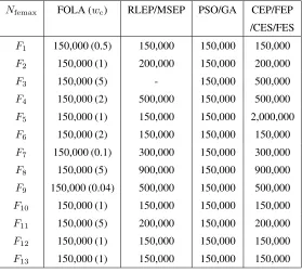
2.1 The setting ofNfemaxfor 30-dimensional benchmark functionsF1_∼F13 45

2.2 Comparison among FOLA and the other eight algorithms on

30-dimensional benchmark functions F1_∼F7: Average fitness value / (Standard deviation) / (Rank) . . . 47

2.3 Comparison among FOLA and the other eight algorithms on

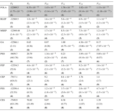
30-dimensional benchmark functionsF8_∼F13: Average fitness value / (Standard deviation) / (Rank) . . . 48

2.4 Comparison among FOLA, GA, PSO, EP and ES on 300-dimensional

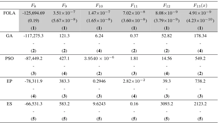
benchmark functionsF8(x)_∼F13(x): Average fitness value / (Stan-dard deviation) / (Rank) . . . 50

2.5 Computation time (s) consumed by PSO, GA, PSO and FOLA when

solving the 30-dimensional benchmark functionsF8(x)_∼F13(x) . . 53 2.6 The average fitness values obtained with differentwcandNfemax . . 54

2.7 Comparison among FOLA, CLPSO and CPSO on 30-dimensional

benchmark functions Frs1_∼Frs9, including Average fitness value, Standard deviation andt-test . . . 56

2.8 Computation time (s) consumed by FOLA, CLPSO and CPSO when

solving the benchmark functions,Frs1(x)_∼Frs9(x). . . 59

2.9 Comparison between FOLA and GS-SOMA on functionsFrs5, Frs6

andFrs8 . . . 62

2.10 Comparison between FOLA and OLPSO on four functions . . . 63

2.11 Comparison between FOLA and SOPEN on 30- and 100-dimensional functionsFrs1andFrs4 without shift and bias . . . 64 2.12 Comparison between FOLA and SOPEN on 100-dimensional

func-tionsFrs1andFrs4 without shift and bias . . . 64 2.13 Comparison between FOLA and SamACO on five benchmark

func-tions . . . 65

3.1 The setting of Nfemin for solving Function I with different

dimen-sionality . . . 85

3.2 The number of non-dominated solutions obtained by MOLA when

wcandNfemaxare set to different values . . . 86

(16)

3.3 The setting of reference solution and extreme solutions; HV and

∆obtained by MOEA/D, NSGA-II and MOLA on Fun1 (including

mean and standard deviation) . . . 94

3.4 The setting of reference solution and extreme solutions; HV and

∆obtained by MOEA/D, NSGA-II and MOLA on Fun2 (including

mean and standard deviation) . . . 99

3.5 D˜, HV and ∆ obtained by MOEA/D, NSGA-II and MOLA on

Fun3-Fun9 (including mean and standard deviation) . . . 106

3.6 D˜ obtained by NSGA-II, MOEA/D and MOLA on Fun10-Fun13

(including mean and standard deviation) . . . 115

4.1 The performance comparison among FOLA, PSO and GA in case 1

on the IEEE 30-bus system . . . 131

4.4 The computation time (s) consumed by FOLA, PSO and GA on the

IEEE 30-bus system . . . 132

4.8 The computation time (s) consumed by FOLA, PSO and GA on the

IEEE 57-bus system . . . 135 4.9 The parameters setting of induction generators . . . 138 4.10 The maximum real power output (MW) of the wind generator in

multiple time periods . . . 138 4.11 The computation time (s) consumed by FOLA, PSO and GA on the

IEEE 30-bus system . . . 141 4.12 The computation time (s) consumed by FOLA, PSO and GA on the

modified IEEE 57-bus system . . . 143 4.13 The minimum fitness values obtained by FOLA, CLPSO and CPSO

in different time periods . . . 146 4.14 Computation time (s) consumed by FOLA, CLPSO and CPSO . . . 146

5.1 The setting of reference solution and extreme solutions;HV and∆

obtained by MOEA/D, NSGA-II and MOLA on the modified IEEE 30-bus power system (including mean and standard deviation) . . . 153

(17)

England test system (including mean and standard deviation) . . . . 155

5.3 Load demand (MW) at bus 10 . . . 155

5.4 Wind speed . . . 156

5.5 The minimum objective fitness values derived by MOEA/D,

NSGA-II and MOLA in the dynamic environment . . . 156

obtained by MOEA/D, NSGA-II and MOLA in dynamic environ-ment: Hours 1-12 (including mean and standard deviation) . . . 158

obtained by MOEA/D, NSGA-II and MOLA in dynamic environ-ment: Hours 13-24 (including mean and standard deviation) . . . . 159

5.8 The wind speed and number of wind turbines in the wind farms . . . 162

obtained by NSGA-II, MOEA/D and MOLA on the modified IEEE 30-bus power system (including mean and standard deviation) . . . 164 5.10 Load demand (MW) at bus 10 . . . 164 5.11 Wind speed for the dynamic IEEE 30-bus power system . . . 164 5.12 The wind speed and number of wind turbines in the wind farms . . . 166

obtained by NSGA-II, MOEA/D and MOLA on the modified new England test system (including mean and standard deviation) . . . . 167 5.14 Wind speed for dynamic new England wind power penetrated system 168 5.15 The computation time (s) consumed by MOEA/D, NSGA-II and

MOLA on the IEEE 30-bus power system . . . 173

(18)

List of Abbreviations and Notations

(19)

Introduction

1.1 Motivations and Objectives

While the mathematics of optimisation has been studied for about a century, the

increasing complexity of real-world optimisation problems and the development of

computation capability have stimulated new interest in the topic. Classical

gradient-based optimisation algorithms have been fully investigated and applied for solving

a wide range of current engineering and public service problems [4]. However,

they are insufficient when solving the multi-model optimisation problems which are

non-differentiable and non-convex and contain many local optima. Furthermore,

their convergence is largely dependent on the initial points of search. To solve these

problems, researchers began to explore the biological evolution and animal

behav-iors in the nature, which serves as a fertile source of concepts, principles and

mecha-nisms. Biologically-inspired optimisation algorithms have thrived over the last few

decades due to their ability of solving multi-modal problems [5], especially

Evo-lutionary Algorithms (EAs), which present their applicability in solving complex

problems. However these algorithms suffer from the drawbacks of redundant

com-putation load and slow convergence rate, i.e. they can hardly achieve an accurate

solution given limited computation time. These drawbacks mainly result from their

population-based search approach, in which there is a high level of randomness and

(20)

1.1 Motivations and Objectives 2

application in large-scale optimisation problems, such as optimal power flow

prob-lems in power systems, routing probprob-lems in telecommunication networks and traffic

systems. Further improvement of EAs is limited. This thesis is concerned with an

alternative approach to function optimisation, based on learning automata.

Nature has presented the significance of learning ability. For instance, in the

wilderness which is full of dangers, each careless action could lead to death, thus

creatures have to learn how to select the actions which are suitable to the

environ-ment. With this inspiration, the feasibility of using a learning method for problem

solving has been explored by researchers [6], such as learning automata methods.

Learning automata methods do not belong to the class of EAs which mainly adopt

biological evolution concept. A learning automaton is considered as a system which

modifies its strategy on basis of its experience by collecting and processing

informa-tion regarding the environment, in order to achieve the desired goal or the optimal

performance in some sense. It is believed that the learning automata, which have

the ability of learning and memorization, can be connected in a way which would

be suitable for tackling complex learning problems. The learning automata methods

have made a significant impact on many areas, such as system control and pattern

classification. They have also been applied to resolve optimisation problems. In

contrast to EAs, the learning automata methods, despite having a solid theoretical

background, are less popularly applied for solving complex optimisation problems.

The objective of this thesis is to discover the potential of Learning Automata

meth-ods (LA) by developing LA-based optimisation algorithms, which can reduce the

unnecessary randomness and large computation load caused by a large number of

population adopted by EAs.

Besides the single objective optimisation mentioned above, multi-objective

opti-misation is with no doubt a very important research topic, due to the multi-objective

nature of many practical optimisation problems in the real world. Multi-objective

optimisation aims to optimise several performance attributes of the problem

simul-taneously and obtains a series of non-inferior alternative Pareto optimal solutions.

There are two standard methods for treating multi-objective problems. One is to

combine the individual objective functions into a single composite function using

(21)

the weighted-sum method or weighted Tchebycheff method. However, the problem

lies with the proper selection of the weights or utility functions to characterize the

decision-maker’s preferences. In practice, it can be very difficult to precisely and

accurately select these weights, even for someone who is familiar with the problem

domain. Small perturbations in the weights can sometimes lead to quite different

solutions [7]. Another drawback of these approaches is that they greatly increase

the computation load, as the algorithm needs to be executed many times in order

to obtain a set of Pareto optimal solutions. In addition, these weighted-objective

methods are only capable of solving convex Pareto front problems and have a

dif-ficulty in solving the multi-objective problems whose Pareto fronts are non-convex

[7]. Nonetheless, there is no way to predetermine if a problem is convex or

con-cave in many applications. Instead of using weighted-sum method, an alternative

is employing Pareto-front based methods, which apply a population of

individu-als, and each of them represents one Pareto optimal solution. These approaches are

extended from EAs, thus they suffer from the same drawbacks regarding

population-based methods, which have been mentioned above. Besides, some of these methods

employ non-dominated sorting strategy to rank the individuals of the population,

which could further increase the computational complexity. This thesis is to develop

an LA-based multi-objective optimisation algorithm, so as to increase the efficiency

of the search, through comprehensively making use of the information collected in

each function evaluation.

Another objective of the thesis is to apply the developed LA-based algorithms

to solve practical problems in power systems. Power system dispatch,

environ-mental concerns and power security are becoming more and more important in

terms of power system operation and planning. These problems are non-differential,

non-linear, high-dimensional and complicatedly constrained. As it is known that

the power system configuration (e.g.power demand, wind power outputs) changes

throughout the whole day, which leads to the varying property of the optimisation

problem. To a certain extent, the property of these problems is unknown in advance,

and it can vary widely as power configuration slightly changes. These features make

(22)

1.2 Optimisation Algorithms 4

suitable for this specific area has not been paid enough attention yet, though some

efforts have been made by researchers who favor EAs. With the high demand of

these problems, the application of EAs is limited in this case, due to their instability

and unpredictable computation load. To overcome this problem, this thesis is also

concerned with the application of LA-based algorithms in complex power systems.

1.2 Optimisation Algorithms

Optimisation refers to systematically finding the optimal solutions to the

opti-misation problems to be resolved, under certain constraints. There are mainly two

categories of optimisation problems, single-objective and multi-objective

optimisa-tion problems. Single-objective optimisaoptimisa-tion problems aim to finding a single best

solution, which is usually the minimal or the maximal evaluation value of the

ob-jective function. On the other hand, multi-obob-jective optimisation problems usually

have no unique, perfect solution, but a series of non-inferior alternative solutions,

Pareto optimal solutions (or called non-dominated solutions), which represent the

possible trade-off among conflicting objectives. The Pareto optimal solutions form

a Pareto front in the objective space. The optimisation target is to find the set of

Pareto optimal solutions which are evenly distributed along the Pareto front [2].

In order to seek the solution which has the best evaluation value of the objective

functions, or a desired combination of two or more optimal fitness values of the

con-flicting objectives, a variety of optimisation algorithms have been developed in the

past century. Classical optimisation algorithms have been largely applied for

solv-ing a wide range of engineersolv-ing and public service problems [4]. However, these

algorithms cannot solve complex multi-model optimisation problems desirably.

Re-searchers began to explore the nature over the past several decades, and develop

var-ious bio-inspired/nature-inspired optimisation techniques, which operate in a rather

different way from the classical methods, and allow scientists and engineers to solve

optimisation problems where the classical methods are not applicable.

(23)

1.2.1 Classical optimisation algorithms

Classical optimisation algorithms, having a solid theoretical background, are

analytical and usually make use of the techniques of differential calculus to locate

the optimum point. They assume that the function is differentiable twice with

re-spect to the design variables, and the derivatives are continuous. Since some of the

practical problems involve objective functions that are not continuous and/or

dif-ferentiable, the classical optimisation techniques have a limited scope in practical

applications. However, classical optimisation algorithms still play an important part

in the field of optimisation. For instance, simplex-based method [8] is a popular

algorithm for numerically solving linear programming problems [9]. Interior point

methods are widely used to solve linear and nonlinear convex optimisation

prob-lems [10][11], which have a convex landscape of the objective functions. In order to

improve convergence rate, many classical optimisation methods are based on

evalu-ating Hessians and gradients [4], such as Newton’s method, Quasi-Newton methods

and steepest descent, and so on. The drawback of these methods is that they increase

the computational cost of each iteration, due to the computational complexity of

evaluating gradients and Hessians.

1.2.2 Evolutionary Algorithms

Since classical optimisation algorithms cannot be used to solve complex

multi-model optimisation problems desirably, a great deal of research activities were

car-ried out from the inspiration of nature [12], and since then, a large number of new

optimisation algorithms have been developed. These methods have been used to

solve various optimisation problems. Meanwhile, these novel optimisation

algo-rithms do not need to run for a large number of times when solving multi-modal

problems, which makes their application efficient. Among these novel

optimisa-tion algorithms, EAs, which incorporate the major behaviours of a biological

evolu-tionary process and a principle of ‘the survival of the fittest’ into their algorithmic

framework [13], have been investigated comprehensively over the last twenty years

(24)

individu-1.2 Optimisation Algorithms 6

als which evolve through iterative process, in order to search for a desired location

in the solution space.

Genetic evolution-based EAs

Genetic evolution-based EAs fall into four major categories: Genetic Algorithm

(GA) [16], Evolutionary Programming (EP) [17], Genetic Programming (GP) [18]

and Evolutionary Strategy (ES) [19]. These methods share the principles of survival

of the fittest.

• The basic concept of GA was first pioneered by John Holland in the 70s [16], and it derives from a metaphor of the evolution process in nature. To be

spe-cific, GA refers to a particular class of EAs that uses the techniques inspired by

evolutionary biology, such as inheritance, mutation, selection, and crossover

[16].

GA is implemented using a population of strings (called chromosomes), which

encode candidate solutions (called individuals) to an optimisation problem,

and evolve towards better solutions [20] [21]. Traditionally, the strings were

in the form of binary values, but later, other forms, such as real-value

cod-ing [22], are also possible [23]. The selection of the type of codcod-ing relates

to the types of the optimisation problem. General GA includes five basic

op-erations: initialisation, selection, crossover, mutation and termination [16].

During the stage of initialisation, a population of individuals are randomly

generated in the solution space. These solutions evolve as generations

pro-ceed. In each generation, the fitness value of each individual in the population

is evaluated. Individual solutions are selected through a fitness-based process,

where the solutions that have better fitness values are often more likely to be

reselected. Some selection strategies rate the fitness value of each solution

and preferentially select the best solutions. However, most selection

meth-ods adopt probability-based selection, in which the probability of reselecting

better solutions is large, and at the same time the solutions which have

rel-atively poor fitness values can also be selected, but in a smaller probability.

(25)

This strategy helps GA preserve population diversity and prevent premature

convergence. The most well-studied selection methods include roulette wheel

selection and tournament selection [24]. Through the stage of selection, an

intermediate population is obtained and used to reproduce a new population.

In this case, multiple individuals are stochastically selected from the current

population to perform operators crossover and mutation. Crossover and

mu-tation are regarded as the main causes of the efficiency of genetic algorithms.

Crossover allows the method to combine some hopeful schemata, join the

information contained in the parent chromosomes, and produce new

individ-uals. With crossover, good results can be obtained with a random matching

of the individuals [22], and thus quickly progress towards the optimal regions

of the search space. On the other hand, mutation brings the diversity among

the population, by changing the values of part of the chromosomes. With the

operations of crossover and mutation, a brand new population is generated,

and it will be used in the next generation. The algorithm either terminates

when a maximum number of generations has been produced, or stops when a

satisfactory fitness level for the population has been reached.

GA can be well extended to solve multi-objective optimisation problems.

Ref-erence [7] provides an overview and tutorial of GA which is developed

specif-ically for problems with multiple objectives. There are mainly two ways of

applying GA in solving multi-objective problems: 1) multiple objectives can

be regulated into a single objective, using weighted-sum method or Lagrange

method, before applying GA. This method is widely used, such as

Weight-Based Genetic Algorithm [25], Random Weighted Genetic Algorithm [26]

and Multi-Objective Genetic Algorithm (MOGA) [7]; 2) being a

population-based approach, a generic single-objective GA can be modified to find a set

of multiple non-dominated solutions in a single run, such as Non-dominated

Sorting Genetic Algorithm [27], Dynamic Multi-objective Evolutionary

Al-gorithm [28] and Fast Non-dominated Sorting Genetic AlAl-gorithm (NSGA-II)

[29].

(26)

experimented and applied in many fields in engineering worlds [21][30][31][32].

A review of their implementations and some application domains can be found

in reference [33].

• EP was first proposed as an approach to artificial intelligence by Fogel in 1960 [17]. However, it was not applied with such a success to many numerical and

combinatorial optimisation problems until 1990 [34].

Similar to GA, EP seeks the optimal solution by evolving the population, in

which each individual represents a candidate solution to the problem, over a

number of generations or iterations. However, unlike other EAs, no

recombi-nation operators are applied in EP. The optimisation process can be

summa-rized into two major steps [17]: the solutions locating in the current population

are mutated; the next generation is selected from both the mutated and the

cur-rent solutions. According to survival of the fittest, the filial generation in EP

is generated from the fittest parent generation which is selected through

rank-ing strategy [35]. Mutation is used to generate new solutions (offsprrank-ing). The

method of mutation could vary dramatically with respect to specific problems,

and it is a critical operation for EP, as it affects the behaviour of individuals

greatly. The contemporary variant, Fast EP (FEP), uses a Cauchy mutation

instead of Gaussian mutation. By introducing the Cauchy mutation, FEP is

more likely to generate an offspring which is far away from its parent, due

to its long flat tails. According to the experimental studies, the improvement

enhances the global search ability of EP [1]. EP does not only conduct the

mutation operation, but also capitalises on a continuous crossover operation

in the evolution process.

EP is comprehensively investigated for multi-objective problems, such as Fast

Multi-Objective Evolutionary Programming [36], which uses fuzzy rank-sum

concept and diversified selection, different multi-objective evolutionary

pro-gramming [37], which has been used for detecting computer network

at-tacks, and Multi-Objective Evolutionary Programming [38], which has been

successfully applied in combined economic emission dispatch and economic

(27)

emission dispatch problems in complex power systems.

• GP is a type of EAs which is on basis of the evolutionary progress

devel-oped by Koza[18]. It can solve various complex optimisations and searching

problems successfully. GP is a domain-independent method that genetically

breeds a population of computer programs to solve a problem. It is an

exten-sion of the GA, but the structures of the population in GP are not fixed-length

character strings used in GA. In GP, the candidate solutions to the problem

[39] are programs, which are expressed in genetic programming as syntax

trees rather than as lines of code. Trees can be easily evaluated in a

recur-sive manner. Every tree node has an operator function, and every terminal

node has an operand, making mathematical expressions easy to evolve and

evaluate. With tree structures representing trial solutions, GP can be applied

to search for the optimal solution, and also used to search for mathematical

functions to describe an unknown model.

The genetic operators used in GP include crossover, mutation, reproduction,

gene duplication, and gene deletion. Mutation affects the population

individ-ually. If one individual is selected to perform crossover, it will simply switch

one of its nodes with another that is from another individual in the population.

With the tree-based representation, it can only replace the node’s information,

or it can replace a whole branch from the selected node. In the latter case,

the crossover is regarded as a replacement of the whole branch. These two

operators are applied to the chromosome in each generation.

• ES was invented in 1963 by Ingo Rechenberg, Hans-Paul Schwefel at the

Technical University of Berlin (TUB) while searching for the optimal shapes

of bodies in a flow [19][40]. ES is a kind of EAs where individuals are

en-coded by a set of real-valued “object variables”. For each object variable, an

individual also has a “strategy variable” which determines the degree of

muta-tion to be applied to the corresponding object variable. The strategy variables

also mutate, allowing the rate of mutation of the object variables to vary. The

(28)

point (parent) and the result of its mutation (child). In each generation, a

vector of object variables is created by mutating the parent with an identical

standard deviation. The fitness value of the child individual is compared with

that of its parent, and the one with the better fitness value survives. This

se-lection mechanism is identified as (1+1)-ES. However, this mechanism may

result in converging to premature results during the optimisation process, due

to a lack of diversity. To overcome this drawback, a multi-membered ES with

µ parents, (µ+1)-ES, was proposed by Rechenberg [41]. In this method, µ

parent individuals can participate in the generation of one offspring

individ-ual. This operation has a similar effect to the crossover process in GA. There

are other ES variants based on this improvement, such as (1+λ)-ES, where

λ mutants are generated from the same parent; (µ+λ)-ES, where the best

µindividuals are produced from the union of parents and offspring (i.e. the selection operates on the joined set of parents and offspring); and (µ, λ)-ES, where only the bestµoffspring individuals are used to form the next parent generation [42].

ES has been applied to solve practical problems in the field of engineering,

such as the optimisation problem in power plant [43].

Swarm intelligence-base EAs

With the exception of the class of EAs which adopts the biological evolutionary

progress, there are also some EAs which are based on swarm intelligence. Swarm

intelligence is the collective behavior of decentralized self-organized systems [44].

These systems are typically made up of a population of simple agents. These agents

follow very simple rules, and no centralized control structure dictates how individual

agents should behave. Although there is no centralized control or the provision of a

global model, agents interact locally with one another and with their environment.

Hence, local interactions between such agents lead to the emergence of “intelligent”

global behavior. These coherent global patterns could be unknown to the individual

agents. A certain degree of randomness is applied to the local interactions between

agents, in order to keep diversity among the swarm. Natural examples of swarm

(29)

intelligence include bird flocking, ant colonies, animal herding, bacterial growth,

and fish schooling,etc.

• Particle Swarm Optimisation (PSO) is a stochastic optimisation technique de-veloped by Eberhart and Kennedy [45][44]. It is inspired by computer

sim-ulations of various interpretations of the movement of organisms in a flock

of birds or a school of fishes. PSO is popular in the research field of

optimi-sation in the last decade for its simplicity of implementation, few parameters

and high convergence rate [46].

In PSO, the population is called a swarm, and each individual of the

pop-ulation is called a particle. PSO works on the social behavior of particles

in the swarm, by remembering the best location of itself and the best

expe-rience of other individuals in the swarm. The particles alter their velocities

according to their records at each iteration. Assume that the search space is

N-dimensional, and the number of particles is np. The position vector and velocity vector of the particlei(i=1,2,. . . ,np) are denoted byZi=(zi1,. . . ,ziN)

andVi=(vi1, . . . ,viN) respectively. The best position of particleiand the fittest

particle found so far in the swarm are represented by P_li=(pli1,. . . ,pliN) and Pg=(pg1,. . . ,pgN) respectively. At each iteration, every component of the

ve-locity vector of particleiis updated according to:

v_ijn+1 =wv_ijn +cf1ζ1(plij ₋zn_ij) +cf2ζ2(pgj₋z_ijn) (1.2.1)

And each component of the position vector is updated according to the

fol-lowing equation:

z_ijn+1 =z_ijn +v_ijn+1 (1.2.2)

wherendenotes the iteration number; wis the inertia weight [47];ζ1 andζ2

are random numbers in the range [0,1]. Constantscf1 andcf2, called accelera-tion factors, are used to adjust particles’ trajectory using its own previous best

position and the best solution found in the group. The velocity obtained from

(1.2.1) makes particles to some extent move towards the global optimum. The

(30)

An important variant of standard PSO utilized a constriction factor, which was

proposed by Clerc [48]. By reducing the inertia weightw in each iteration, it ensures the stability of convergence, and it leads to higher quality of the

solutions compared with the standard PSO when solving unimodal functions,

which have only one local minimum. However, an over-decreased inertia

weight reduces the velocity of particle,i.e., the particle is trapped more easily

at local optima in multimodal optimisation problems which have a number

of local optima. Other variants of the PSO have also been developed in

re-cent years, such as Particle Swarm Optimisation with Passive Congregation

[49], Unified Particle Swarm Optimisation, Fully Informed Particle Swarm

and most recently, Cooperative Particle Swarm Optimisation (CPSO) [50] and

Comprehensive Learning Particle Swarm Optimisation (CLPSO) [51]. These

algorithms have produced encouraging results in both benchmark testing and

real-world applications.

• Ant colony optimisation algorithm (ACO) is another approach which is based

on swarm intelligence [52]. It models ant colony behaviour, including ant

foraging behaviour, brood sorting, nest building, and self-assembling. Ants

wander randomly, and deposit pheromone trails on the way back to the colony

after finding food. If other ants find a pheromone path, they are more likely

to discontinue their random travel, and follow the trail until reaching the food

source. Subsequently, they reinforce the pheromone trails. The pheromone

trails evaporate with time, resulting in a reduction of the strength of attraction.

This process is simulated by ACO to find an optimal solution.

ACO has been applied to many combinatorial optimisation problems, in which

the set of feasible solutions is discrete or can be reduced to discrete. Taking

Traveling Salesman Problem (a popular combinatorial problem) as an

exam-ple, the solution obtained by ACO is much better than the one found by a GA

[53]. After more than ten years of studies, both its application effectiveness

and its theoretical background have made ACO a successful EA in the

com-binatorial optimisation domain [54]. Besides, the applications of ACO range

from quadratic assignment to protein folding and vehicles routing. A number

(31)

of derived methods have been adopted to solve dynamic problems, stochastic

problems, multi-targets and parallel implementations [55].

• Recently, a Group Search Optimiser (GSO) was developed at the University of Liverpool [56], which was inspired by animal searching behaviour and group

living theory [57]. The strategies of information-sharing [58] and

producer-scrounger models [59] are employed in GSO. There are mainly three roles in

a group: producer, scrounger and ranger. Producer, regarded as the leader of

the group, is usually located in promising area, and seeks food source for the

rest of the group. There is only one producer in the group. In each iteration,

the producer is renewed and are selected from the best members. On the other

hand, scroungers follow the producer and find opportunities to share the

infor-mation found by producer and search resource uncovered by other scroungers.

Apart from the producers,80%of the rest members are randomly selected as

scroungers, and the scroungers are renewed in each iteration as well. The

re-mainder members are rangers. They walk randomly in the searching space, by

dispersing themselves from their original positions. This behavior increases

the diversity in the group, and discourages members from being trapped in

local optima. Concepts from this framework are employed metaphorically

to design optimum searching strategies for solving continuous optimisations.

GSO is extended to solve objective optimisation problems using

multi-ple producers. Scroungers search around one of the producer and one of the

non-dominated solutions. The number of the producers is equal to that of the

objective functions. This method has been successfully applied to solve the

problem of device placement in power systems [60].

1.3 Introduction to Learning Automata

The first learning automaton model was developed in mathematical psychology,

and then developed by Bushet al. [61], Atkinsonet al. [62] and Tsetlin [63]. Learn-ing automata select their current actions based on past experiences learned through

(32)

collect-1.3 Introduction to Learning Automata 14

ing and processing current information regarding the environment, be capable of

changing their structure and parameters as time evolves, in order to achieve the

de-sired goal or the optimal performance. The learning automata methods have already

made a significant impact on many areas of system control and pattern classification,

such as power system control [64][65], vehicle suspension control [66] and

noise-tolerant learning of hyperplane classification [67],etc. They have also been inves-tigated in solving optimisation problems. For instance, the method of

continuous-action learning automata has been applied for stochastic optimisation [68][69]; the

algorithm of genetic learning automata was proposed to resolve function

optimi-sation problems [70][71]. However, few literature has reported that the learning

automata methods, despite having a solid theoretical background, can outperform

EAs in solving complex optimisation problems, particularly for high-dimensional

optimisation problems. In addition, they have also been applied to solve

objective optimisation problems [72], but only limited in low-dimensional

multi-objective problems.

1.3.1 Basic elements

A general block diagram of the interaction between environment and an

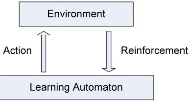
automa-ton is provided in Fig. 1.1.

Environment

Learning Automaton

[image:32.612.212.406.440.543.2]

Reinforcement Action

Figure 1.1: Block diagram of the interaction between a Learning Automaton and environment

The learning process of learning automata can be simply described as follows

[73]: during the interaction with environment, the automaton randomly selects an

action from the action set that includes the possible actions the automaton can take

(33)

at its current state, based on a probability distribution. The probabilities of

select-ing the actions are the same initially. Then the environment generates a response to

the action, named reinforcement signal. According to the response, the automaton

updates the action probability distribution. The algorithm used to update the action

probabilities is called the learning algorithm or reinforcement scheme. Afterwards,

a new action is selected according to the updated probability distribution. Regarding

this action, a response is elicited by the environment, and the procedure is repeated.

It can be seen that the implementation of learning automata mainly concentrates

on three aspects: how to select actions, learning algorithm and reinforcement

sig-nal, as given in Fig. 1.2. Unlike EAs that mainly apply the concept of biological

evolutionary concept, learning automata methods are based on action selection and

probability distribution.

LA

Action

selection algorithmLearning Reinforcement signal

Figure 1.2: The three aspects of LA

The automaton

The state X X={X ,X,,X

}

Input set R R={r,r,,r }

or {( ′ ′)}

Output set A A={a,a,,a

}

Transition Function F

Output function G

Figure 1.3: The illustration of an automaton

A learning automaton is an adaptive decision-making unit situated in a random

environment. The learning automaton learns the optimal action through repeated

interactions with its environment. The illustration of an automaton is given in Fig.

1.3. Being an adaptive discrete machine, an automaton can be described as:

(34)

1.3 Introduction to Learning Automata 16

These entities are described precisely as follows:

• Thestateof the automaton at instantn, denoted byX(n), is an element of the finite set:

X =_{X1, X2, . . . , XXN_} (1.3.2)

• The output or action of an automaton at instant n, denoted by a(n), is an element of the finite set:

A=_{a1, a2, . . . , aaN_} (1.3.3)

• The input to an automaton at instantn, denoted byr(n), is an element of a set

R, which could be either a finite set or an infinite set, such as an interval on the real line. Thus,

R =_{r1, r2, . . . , rrN_}orR=_{( ˜α,β˜)_} (1.3.4)

whereα˜andβ˜are real numbers.

• The probability of choosing actioniat instantn, denoted bypi(n), is an ele-ment of the finite set:

P =_{p1, p2, . . . , paN_} (1.3.5)

• F(_·,_·) is transition function, which determines the state at instant (n + 1) regarding the state and input at instantn:

X(n+ 1) =F[X(n), r(n)] (1.3.6)

or F is a mapping from X _×R _→ X. F could be either deterministic or

stochastic.

• Output functionG(_·)determines the output of the automaton at any instantn

according to its current state:

a(n) =G[X(n)] (1.3.7)

orGis a mappingX _→A. It is again either deterministic or stochastic.

(35)

• T represents the reinforcement scheme (learning algorithm), which deter-mines the action probabilities at instantn + 1 regarding the probabilities at instantn:

p(n+ 1) =T[p(n)] (1.3.8)

Basically, the automaton takes in a sequence of inputs and outputs a sequence

of actions with respect to the observation time n. The working of an automaton

can be described as follows: given an initial stateX(0), actiona(0)is determined by functionG. Based on current state, the response generated by the environment,

r(0), and the transition function determine the next state X(1). These operations are performed recursively, and in this way, the state sequence and action sequence

are obtained according to any given input sequence [74].

In terms of functionsFandG, there are two types of automaton:

• Deterministic automaton. For this automaton, functions F and G are both

deterministic mappings. It means that with a given initial state and a given

input, the succeeding state and action are uniquely specified. The mappings

of the two functions can be represented either in the form of matrices or graphs

if the input set is finite. Corresponding to each input, the matrix or the graph

can indicate how the present state transfers to a new state. In this case, the

transition matrices consist of elements that are only either 0 or 1.

• Stochastic automaton. For this automaton, at least one of the functionsFand

G is stochastic. In other words, given an initial state and an input, there is

no certainty concerning the succeeding state and action, which are associated

with probabilities. If transition functionFis stochastic, given the present state

and input, the next state is at random, andFgives the conditional probabilities

(or called transition probabilities) of reaching the various states. If the output

functionGis stochastic, given the present state, the action taken is at random

and is determined by the conditional probabilities provided byG.

(36)

transition matrix are constants which take values in the interval [0,1], and each

transition matrix is a stochastic matrix. On the other hand, if the transition

probability at instantnis updated on the basis of the input at that instant, the automaton is called a variable-structure stochastic automaton. The elements

of the transition matrix are in [0,1], but they are no longer constants any more,

as they are updated withn.

The environment

Environment refers to the aggregate of all the external conditions and influences

which would affect the automata [74]. The role of the environment is to establish

the relationship between the actions taken by the automaton and the signal inputs

to the automaton [69]. An environment can be mathematically defined as a triple

{A, C, R_}. A represents a finite input set. R represents the output set, i.ethe en-vironment’s response to the action taken by the automaton. The environment is

referred to as aP-model environment when its response belongs to the binary set

{0,1_}; the environment is named asS-model environment when its response takes an arbitrary value in the closed segment [0,1]; Q-model environment refers to the environment whose response is one of a finite number of values in the interval [0,1].

The environment is characterized by C, which represents the penalty probability,

i.e.the likelihood that the application of an action to the environment will result in a penalty output. If the penalty probabilities are constant, the environment is said to

be stationary; otherwise, it is nonstationary.

Reinforcement schemes

Reinforcement schemes are the methods used to update action probabilities at

each instant. They were originally proposed to model animal learning [61], but later

it was found that they can be applied in the field of learning automata successfully.

Choosing reinforcement scheme is a crucial factor that affects the performance of

learning automata [75]. In general, a reinforcement scheme can be represented by:

p(n+ 1) =T[p(n), r(n), a(n)] (1.3.9)

(37)

whereTis a learning operator;r(n)anda(n)represent the input to the automaton and the action taken by the automaton at instantn, respectively.

The basic idea behind a reinforcement scheme can be described as follows: if

the automaton selects an actionai at instantnand receives a nonpenalty input, the action probability of the actionai,i.e. pi(n), will be increased, and the probabilities for all other actions will be decreased. In this case, the change occurring onpi(n)is

called reward. For a penalty input,pi(n)is decreased and other action probabilities are increased. At this moment, the change applied onpi(n)is called penalty.

If pi(n + 1)is a linear function of pi(n), the reinforcement scheme can be de-scribed as linear, such as Linear Reward-Inaction (LR−I) algorithm [74], which is

known to be very effective in many applications. TheLR−Iupdates the action

prob-abilities as follows (assuminga(n) =ai):

pi(n+ 1) =pi(n) + ˜λr(n)(1₋pi(n))

pj(n+ 1) =pj(n)₋λr˜ (n)pj(n), for allj ₆=i (1.3.10) On the other hand, if pi(n+ 1)is a nonlinear function ofpi(n), the reinforcement scheme is said to be nonlinear. Several non-linear schemes have been suggested by

Viswanathan and Narendra [76], Lakshmivarahan and Thathachar [77]. Sometimes,

it is advantageous to use different schemes to update pi(n), while the selection of

the reinforcement scheme depends on the intervals the value ofpi(n)lies in.

1.3.2 Several learning automata methods

Although each individual of the learning automata is an independent unit in a

simple structure, a group of learning automata can be connected in a way which

would be suitable for tackling complex learning problems. Systems built with LA

have been successfully employed in many difficult learning situations over the years.

This has also led to the concept of LA being generalized in a number of directions,

(38)

Finite Action-set Learning Automaton (FALA)

The original notion of learning automaton is derived from what is called finite

action-set learning automaton (FALA) [74]. FALA is the learning automaton for

which the number of possible actions is finite,i.e.the size of the action-set is finite. This type of learning automaton has been studied extensively.

A learning automaton is an adaptive decision-making device that learns the

op-timal action out of a set of actions through repeated interactions with a random

environment [78], as described in Section 1.3.1. There are two characteristics of the

learning automata: 1) the action choice is based on a probability distribution over

the action-set; 2) and the probability distribution is updated at each instant based on

the reinforcement feedback from the environment.

The operation of FALA consists of repetitions of the following several steps:

choosing action randomly, receiving reinforcement from environment and updating

action probability. The process can be specifically described as follows: at each

instantn, the automaton chooses an actionarandomly, based on its current action probability distribution,p(n) = (p1(n), . . . , paN(n))T_{, where}_pi₍_n_{) = prob[}_a₍_n_{) =} ai]andPaN

i=1pi(n) = 1,∀n. The action chosen by the automaton is the input to the

environment. The environment responds to the action with a stochastic reaction or

reinforcement, r(n), which is the input to the automaton. The higher the value of the reinforcement signal, the more desirable the action. Let

Fi =E[r(n)_|a(n) = ai], i= 1, . . . , aN (1.3.11)

Fi is often referred to as reward probability of action ai. Define an index I by

FI = max_{Fi_}. Then the action aI is called the optimal action. The learning automaton has no knowledge of the reward probabilities. The automaton’s objective

is to identify the optimal action. The goal is achieved through a learning algorithm

that updates, at each instantn, the action probability distributionp, through the most recent interaction with the environment, namely, using the pair_{a(n), r(n)_}.