City, University of London Institutional Repository
Citation:
Cowell, R. (2009). Efficient maximum likelihood pedigree reconstruction.
Theoretical Population Biology, 76(4), pp. 285-291. doi: 10.1016/j.tpb.2009.09.002
This is the accepted version of the paper.
This version of the publication may differ from the final published
version.
Permanent repository link:
http://openaccess.city.ac.uk/6014/
Link to published version:
http://dx.doi.org/10.1016/j.tpb.2009.09.002
Copyright and reuse: City Research Online aims to make research
outputs of City, University of London available to a wider audience.
Copyright and Moral Rights remain with the author(s) and/or copyright
holders. URLs from City Research Online may be freely distributed and
linked to.
City Research Online:
http://openaccess.city.ac.uk/
[email protected]
Efficient maximum likelihood pedigree reconstruction
Robert G. Cowell
Faculty of Actuarial Science and Insurance, Cass Business School, 106 Bunhill Row, London EC1Y 8TZ, UK
Abstract
A simple and efficient algorithm is presented for finding a maximum
likeli-hood pedigree using microsatellite (STR) genotype information on a complete
sample of related individuals. The computational complexity of the algorithm
is at worst (O(n3
2n)), wherenis the number of individuals. Thus it is possible
to exhaustively search the space of all pedigrees of up to thirty individuals for
one that maximizes the likelihood. A priori age and sex information can be
used if available, but is not essential. The algorithm is applied in a simulation
study, and to some real data on humans.
Key words: Pedigree reconstruction, Bayesian network, maximum likelihood
1. Introduction
There are a number of situations in which reconstructing the pedigree of
re-lated individuals from genetic data is of interest and importance, both in human
and non-human populations. Biologists interested in (preserving) endangered
species may have an interest in pedigree reconstruction, as it may help in
infer-ring the population size, and the amount of inbreeding within the species. This
in turn could help to determine both the genetic variability and viability of the
species.
Mass-grave scenarios, or disasters in which the remains of many people are
found and can only be identified by DNA profiles, can also lead to the
lem of reconstructing pedigrees. A quite famous historical case concerns that
of the Russian royal family who disappeared during the Russian revolution of
1917. In July 1991, in a shallow grave 20 miles from Ekaterinburg, Russia, nine
skeletons were found. From the size of some of the bones three were identified
as children. The remains were believed to be the remains of Tsar Nicholas II,
his wife, three of their five children, together with some servants, and the Royal
Physician. A sophisticated DNA analysis of the remains, including comparison
of mitochondrial DNA obtained from the remains to that obtained from blood
donated by the Duke of Edinburgh (a grand-nephew of the Tsarina) confirmed
the identification of the members of the Romanov family (Gillet al., 1994).
One approach to pedigree reconstruction using genotypic data is to find the
pedigree having the maximum likelihood. This was developed by Thompson
(1976) (see also (Thompson, 1986)) using age and sex information, and more
recently by Almudevar (2003) who presented a simulated annealing algorithm
that can run either with or without age and sex information. Both of these
authors used acomplete sample of individuals. This means that a parent of an
individual is either in the sample, or if not he or she is unrelated to all other
members in the sample. Under this assumption, the likelihood function for a
given pedigree decomposes into a simple multiplicative form: this paper will
also assume a complete sample. For recent reviews of pedigree reconstruction,
see Jones and Ardren (2003) and Blouin (2003).
In recent yearsBayesian network expert systems (Cowellet al., 1999) have
been applied to model and analyse problems of forensic genetics. Dawidet al.
(2002) describe how to use Bayesian networks to analyse problems of disputed
paternity. Mortera (2005) and Cowell et al. (2007) have developed Bayesian
networks to analyse mixed DNA samples, such as may be found at a crime
scene. Lauritzen and Sheehan (2003) provide an overview of various Bayesian
network representations for genetic modelling applications.
Within the Bayesian network community there has been much work in
in-ferring Bayesian network structure from data; see, for example, Cooper and
pedi-gree from genotypic data is similar to learning a Bayesian network from data,
though the latter tends to be more complex. This is because the graphical
struc-ture of a pedigree is constrained so that an individual has at most two parents,
and if sex information is available, they are of opposite sex. This considerably
reduces the number of possible pedigrees on n individuals, compared to the
number of Bayesian networks onnnodes; nevertheless the number of pedigrees
still grows rapidly withn.
Following on from work by Koivisto and Sood (2004), a Bayesian network
structure learning algorithm capable of searching the complete space of Bayesian
networks for up ton= 25 variables was proposed by Singh and Moore (2005).
Subsequently a simpler and more efficient (and currently state-of-the-art)
algo-rithm was proposed by Silander and Myllym¨aki (2006) that is able construct
maximum scoring Bayesian networks with up to 32 variables. In this paper
the latter algorithm is specialised and adapted to the purpose of reconstructing
pedigrees using a complete sample. The algorithm is efficient—finding the
max-imum likelihood pedigree with 20 individuals takes around 1 second, whilst with
29 individuals the time rises to just over 8 minutes.1
Previously, an exhaustive
search over all pedigrees on more than nine individuals would have been
pro-hibitive (Egeland et al., 2000). As the complexity is similar to the Bayesian
network learning algorithm of Silander and Myllym¨aki (2006), the pedigree
re-construction algorithm proposed in this paper will also be feasible for up to 32
individuals, the limit they suggest for their algorithm.
The plan of the paper is as follows. In the next section the pedigree
re-construction algorithm is presented. It is then applied in a simulation study
of two pedigrees involving 20 individuals, and also to the Romanov mass grave
dataset. The discussion section examines limitations of and potential uses and
extensions of the current work.
1
All timings refer to calculations carried out using a computer with an AMD dual-core
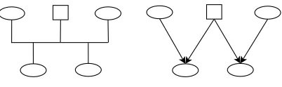
Figure 1: A simple pedigree showing two female half siblings, each of their mothers and their
common father, using a standard pedigree diagram (left) and a Bayesian network
representa-tion (right).
2. The search algorithm
2.1. The likelihood function
We shall represent a given pedigree on n individuals of known genotype
graphically using a Bayesian network, in which each node represents the
geno-type of an individual. If A and B are nodes in the network, then a directed
edge fromA to B means thatA is a biological parent ofB. Figure 1 shows a
simple pedigree for two half siblings and their parents as a Bayesian network.
One property of the Bayesian network is that it is adirected acyclic graph. This
means that you cannot start from some node, follow a path along edges in the
directions of the arrows, and arrive back where you started. Biologically this
corresponds to the logical requirement that an individual cannot be her/his own
ancestor.
Suppose we have a given pedigree Bayesian network structureG, consisting
of nodesV and directed edge setE, where each node represents the genotype of
an individual, and the genotypes of all individuals are known. Then each node
ofGhas one of three possible parent configurations:
• The node has no incoming arrows. Hence the individual is a founder in
the pedigree.
• The node has one incoming arrow. Hence the individual has only one
parent specified in the pedigree.
• The node has two incoming arrows. Hence both parents of the individual
Let V0 denote the set of nodes that have no incoming arrows,V1 the set
of nodes that have one incoming arrow, and V2 denote the set of nodes that
have two incoming arrows. Then following Almudevar (2003), we letα1(gi|gj)
denote the conditional probability that individuali∈ V1 has genotypegi given
one of its parents j ∈ V has genotype gj. Similarly, α2(gi|gj, gk) denotes the
conditional probability that individuali∈ V2has genotypegigiven that its two
parents j, k have genotypes gj and gk respectively. We let α0(gi) denote the
(marginal) probability that individuali∈ V0 has genotypegi.
We shall assume Hardy-Weinberg equilibrium, so that the founders in the
pedigree are unrelated (or marginally independent, in the Bayesian network
terminology). Then, under the assumption of a complete sample, the likelihood
of the pedigreeGdecomposes into the product
L(G) =L0(G)L1(G)L2(G),
where
L0(G) =
Y
i∈V0
α0(gi),
L1(G) =
Y
i∈V1
α1(gi|gj),
L2(G) =
Y
i∈V2
α2(gi|gj, gk).
For simplicity we shall also assume in the examples later in the paper that the
STR markers in the marker system that specifies the genotypes are independent
(unlinked), and that mutation does not take place. Under these extra
assump-tions, the likelihood termsLi(G) factorize further, as described by Almudevar
(2003). (The algorithm presented in the next section does not require these
additional assumptions, but it does require that the variousαprobabilities can
be evaluated.)
Without loss of generality, we shall label the|V|individuals with the integers
1,2, . . . , n, and use the index 0 to represent a general “absent” individual. Then
we may write, fori, j andk∈ {1, . . . , n}:
α1(gi|gj) ≡ α2(gi|gj, g0) =α2(gi|g0, gj)
We shall also work with the log-likelihood rather than the likelihood. Thus the
log-likelihood may be written as
l(G) = logL(G) =
n
X
i=1
logα(gi|gj, gk) (1)
where either or both parents j and k of individual i can take index value 0,
indicating untyped individuals not (explicitly present) in the pedigree, and the
suffix 2 ofα2(∗|∗,∗) is now superfluous and so has been omitted.
Note, importantly, that the log likelihood is decomposed into a sum of terms,
with one term from each of then individuals.
2.2. Overview of the reconstruction method
As mentioned in Section 1, the pedigree reconstruction algorithm presented
here is based on the method of Silander and Myllym¨aki (2006). It is, however,
simpler because within a pedigree an individual can have at most two parents,
whilst in a Bayesian network a node can have more than two incoming arrows.
The key observation, also used by Singh and Moore (2005), is that in a directed
acyclic graph there is at least one node, called aterminal node orsink, that does
not have any outgoing edges. In a pedigree, this will be true for the youngest
individual. Removing this sink node results in a directed acyclic graph that also
has a sink node.
So suppose that we havennodes in a set V to begin with, labelled from 1
ton. For each nodei∈V we can find the the combination of parents in V \i
that maximizes the contributionα(gi|?,?) to the log likelihood (1). If we could
also find for each of thensetsV \i:i= 1, . . . , n, each ofn−1 individuals, the
maximizing value of the log likelihood over all pedigrees—call thisl(V\i)—then
we can identify the “best” or optimum sink as that nodeiwhich maximizes the
sum logα(gi|?,?) +l(V\i). Having found the “best sink” with the “best score”,
a pedigree search can then be carried out on the remainingn−1 individuals.
search algorithm. Silander and Myllym¨aki (2006) instead use an array in which
best scores and sinks are stored and updated as they are encountered during
the execution of their algorithm. A key requirement is that the score function
is decomposable, which is true of the pedigree likelihood function used here.
2.3. Details of the reconstruction method
There are four main steps to the pedigree reconstruction algorithm.
1. Find the set of possible parent configurations for every individuali.
2. Find the best sinks for all 2n subsets ofV.
3. Find a best ordering of best sinks.
4. Recover the pedigree using the sink ordering and the best parents of each
sink.
The details are as follows:
Step 1: Finding local score contributions.
In this a list Λi is constructed for each individual i ∈ V that stores the
combinations of possible parents and the corresponding local scoresα(i|j, k).
• For eachi ∈V and all the valid (j, k) parent combinations (with j < k
or j = k = 0) that i can have using the remaining variables V \i, find
the corresponding score contributionα(i|j, k)>0, and store the ordered
quadruple (α(i|j, k), i, j, k) in the list Λi.
• Sort each list Λiin decreasing order of the score contributionα(i|, j, k) of
the quadruples.
Note that each list Λi always has at least one element, corresponding to
j=k= 0 which treats ias a founder, and that the probabilities stored are all
strictly positive. Genetic constraints will usually make the number of elements
in each list small if there is no mutation, but with mutation, the lists can have
up to 1 +n(n−1)/2 entries. (These arise as follows: (n−1)(n−2)/2
the founder entry α(i|0,0).) Hence this part of the algorithm has complexity
O(n3
).
Step 2: Finding best sinks
This is the heart of the algorithm, and where the computational complexity
is greatest. We use two arrays,scores[] andsinks[], each of size 2n, with each
element corresponding to a subset ofV. The algorithm proceeds by examining
the subsets of V in a particular order: two possible orderings are presented
here. In addition, there is a lookup procedure that finds the best parents for an
individualifrom any subset ofV and returns the associated Best Local Score:
this will be denoted byBLS(i, W) whereW ⊆V\i. It also uses a local variable
skore. On completion of this step of the algorithm, the arraysinks[] stores for
each subset ofV the best sink.
• For allW ⊆V in ORDER Do
> scores[W]←0.0
> sinks[W]← −1
• For alli∈W Do
> U ←W\ {i}
> skore←BLS(i, U) +scores[U]
• Ifsinks[W] =−1 orskore > scores[W] Then Do
> scores[W]←skore
> sinks[W]←i
Finding the Best Local Score BLS(i, U) is straightforward. One simply
traverses the sorted list Λi inspecting the quadruples (α(i|j, k), i, j, k) in turn.
The first quadruple encountered such that j ∈ U and k ∈ U gives the best
parent set for individuali out of the subset of individualsU, and log(α(i|j, k))
is the corresponding value ofBLS(i, U). (Note that 0⊆U always.)
The heart of the algorithm is in using an appropriate ORDER. What we
the best scores of all subsets U ⊂W have already been evaluated and stored
in elements of scores[], and so can be accessed readily without recalculation.
One possible ordering that achieves this is to look at the subsets in an
or-der of non-decreasing size, starting with the empty set. For example, suppose
we have three individuals, then the sequence of subsets W of V consisting of
∅,{1},{2},{3},{1,2},{1,3},{2,3},{1,2,3}will work.
An alternative, used by Silander and Myllym¨aki (2006), is to use a
lexico-graphic order of bit vectors that implement the sets. Treating the case of three
individuals once more, the ordering would be: {}= 000,{1}= 001,{2}= 010,
{2,1}= 011,{3}= 100,{3,1}= 101,{3,2}= 110 and{3,2,1}= 111. This is
simple to implement, as it corresponds to counting from 0 to 2n−1 in binary
and the count variable can be used as the array index.
This step of the algorithm has the greatest computational complexity. In the
worst case the complexity of callingBLS(i, U) is O(n2
). For a givenW ⊂V,
theForloop is called 1≤ |W| ≤ntimes. Hence eachForloop call has worst
case complexity ofO(n3
), and is called for each of the 2n subsets ofV. Hence
the worst case running time complexity of the algorithm is O(n3
2n), but will
typically be much less than this (but still at leastO(2n)). It also requires an
array of size 2n to store thescore[] values in memory. If memory storage is an
issue, then the array sinks[] may be written to a file as generated instead of
being stored in an array in memory: the values can re-read into memory for the
Steps 3 and 4, for which thescores[] array is not required.
Step 3: Ordering the sinks
After Steps 1 and 2, the arraysinks[] stores the best sink for each subset
ofV. So the algorithm first finds the best sinki forV, then the best sink for
V \ {i}, etc. The algorithm is the same as in Silander and Myllym¨aki (2006),
and uses an integer arrayord[1, . . . , n].
• Initializelef t={V}.
> ord[i]←sinks[lef t]
> lef t←lef t\ {ord[i]}
At the end of the algorithm, the arrayord[] is a permuted ordering of then
individuals, withord[1] being a founder andord[n] being a childless individual
in the maximum likelihood pedigree. With the arraysinks[] in memory, the
complexity is linear inn.
Step 4: Recovering the pedigree
The final step is to extract the pedigree from the ordering. It uses a lookup
functionBLSet(i, U) that is identical to the score functionBLS(i, U) of Step 2,
but returns the parent set (j, k) instead of the scoreα(i|, j, k). This step also uses
an arrayparents[1, . . . , n] of sets, a local set variable predecsof predecessors,
and theord[] array from Step 3.
• predecs← ∅
• Forifrom 1 step 1 tonDo
> parents[ord[i]]←BP Set(ord[i], predecs)
> predecs←predecs∪ {ord[i]}
At the end of the algorithm the array elementparents[i] contains the parent
set for the individual i. Taken together for all individuals i ∈ [1, . . . , n], this
defines a pedigree having the maximum likelihood. (Note that there could be
more than one pedigree that achieves the same maximum likelihood value.)
3. Evaluation and results
3.1. Example 1: Simulation using two pedigrees
Figure 2 and Figure 3 show two pedigrees each with twenty individuals, the
second highly inbred, that were used in a simulation study. Genetic profiles for
all individuals were simulated using the assumptions of Hardy-Weinberg
equilib-rium, independence of markers and no mutation. Four pedigree reconstruction
Figure 2: A pedigree of twenty individuals with slight inbreeding. Note that the offspring of
individual 7 are all half-siblings, as are the offspring of individual 12.
[image:12.595.204.409.421.612.2]• Use 10 markers, without sex information
• Use 10 markers, using sex information
• Use 15 markers, without sex information
• Use 15 markers, using sex information
In both pedigrees, in using sex information, the even numbered individual were
assigned as male, and the odd numbered individuals as female.
Allele frequencies were taken for the American Caucasian population given
by (Butleret al., 2003). For the first two scenarios, the following markers were
used: CSF1PO, FGA, THO, TPOX, VWA, D3, D5, D7, D8, and D13. The
following additional five markers were used for the second pair of simulations:
D16, D18, D21, D2 and D19. None of the simulations used age or generational
information from the true pedigree. For each scenario, 1000 genetic profiles for
the individuals were simulated. Both the likelihood of the profile according to
the true pedigree, and the maximum likelihood were found. Typically it took
approximately 1.1 seconds to find the maximum likelihood pedigree for each
pedigree profile.
Figures 4 and 5 show the distribution of the differences in the log-likelihood
of the true pedigree and the value obtained for the maximum log-likelihood,
(that is, the log-likelihood ratio), for the subsets of simulations for which the
difference is non-zero, that is, when the algorithm found a pedigree having a
higher likelihood than the true pedigree. (The logarithms are to base-10 in all
plots.) As is to be expected, as the number of markers is increased, and also
in-formation about the sex of individual is used, the number of times the maximum
likelihood exceeds the likelihood of the true pedigree decreases. We also see on
the plots the excess values bunching closer to zero. Perhaps surprisingly the
re-construction algorithm appears to perform better on the highly inbred pedigree
of Figure 3 than the pedigree of Figure 2 when comparing the excess totals in
each scenario. This might be because in the highly inbred pedigree, apart from
No sex information, 10 markers: 849
Excess of log likelihood
Frequency
0 2 4 6 8 10
0 50 100 150 200 250
Sex information, 15 markers: 847
Excess of log likelihood
Frequency
0 2 4 6 8 10
0 50 100 150 200 250
No sex information, 15 markers: 613
Excess of log likelihood
Frequency
0 1 2 3 4 5
0 100 200 300 400 500
Sex information, 15 markers: 602
Excess of log likelihood
Frequency
0 1 2 3 4 5
[image:14.595.144.457.254.469.2]0 100 200 300 400 500
Figure 4: Simulation results for pedigree in Figure 2. The histograms shows the distribution
of the difference of the maximum log-likelihood value and the log-likelihood value according to
the true pedigree, for the subset of simulated profiles for which these quantities were different.
(That is, the log10likelihood ratio between the maximum-likelihood and true pedigree.) The
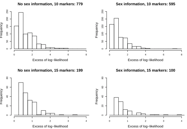
No sex information, 10 markers: 779
Excess of log−likelihood
Frequency
0 2 4 6 8
0 50 100 150 200 250
Sex information, 10 markers: 595
Excess of log−likelihood
Frequency
0 2 4 6 8
0 50 100 150 200 250
No sex information, 15 markers: 199
Excess of log−likelihood
Frequency
0 1 2 3 4
0
20
40
60
80
Sex information, 15 markers: 100
Excess of log−likelihood
Frequency
0 1 2 3 4
0
20
40
60
[image:15.595.145.472.250.475.2]80
Figure 5: Simulation results for pedigree in Figure 3. The histograms shows the distribution
of the difference of the maximum log-likelihood value and the log-likelihood value according to
the true pedigree, for the subset of simulated profiles for which these quantities were different.
The caption of each histogram gives the total number of such different values from 1000
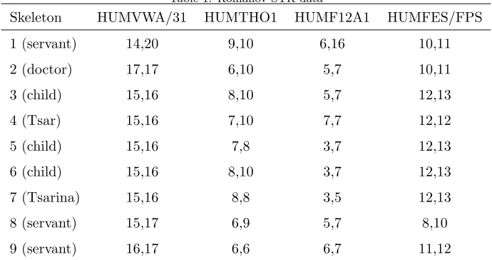
Table 1: Romanov STR data
Skeleton HUMVWA/31 HUMTHO1 HUMF12A1 HUMFES/FPS
1 (servant) 14,20 9,10 6,16 10,11
2 (doctor) 17,17 6,10 5,7 10,11
3 (child) 15,16 8,10 5,7 12,13
4 (Tsar) 15,16 7,10 7,7 12,12
5 (child) 15,16 7,8 3,7 12,13
6 (child) 15,16 8,10 3,7 12,13
7 (Tsarina) 15,16 8,8 3,5 12,13
8 (servant) 15,17 6,9 5,7 8,10
9 (servant) 16,17 6,6 6,7 11,12
In contrast, in the other pedigree, there are 4 founders, (1,2,3 and 5) and two
groups of three half-siblings (13,14,15) and (18,19,20). However the distribution
of excess values appears concentrated closer to the origin in the pedigree with
only a slight amount of inbreeding.
3.2. Example 2: The Romanov family
Table 1 shows STR genotype data for the nine skeletons found in a shallow
grave 20 miles from Ekaterinburg, Russia, and believed to be the remains of
the Romanov family, some servants and the family doctor (Gill et al., 1994),
described in Section 1. Five of the individuals including all the children were
female, the remaining four individuals were male.
Two pedigrees reconstructions were carried out, one using sex information
the other not. In both cases age information was not used. In the absence of
suitable population allele frequencies, each marker was assumed to consist of
eight alleles, (inclusive of the ones in the table), with a uniform distribution.
Figure 6 shows the maximum likelihood pedigree that results without using the
sex information. Although the pedigree places the members of the Romanov
family in the correct group, the relationships are incorrect. Using age
have been ruled out. Using the sex information would also rule this out, as the
children were all female. Using sex information2
gives the pedigree in Figure 7,
in which the royal family group is now correctly established. Note that both
reconstructions suggest that the doctord2 is related to two of the three servants.
Pedigrees in whichs9 is the father of the doctor, and the doctor is the parent of
s8, or in whichs8 ands9 are half siblings with the doctor as the common
par-ent, would be equally likely. However, these familial relationships between the
doctor and the two servants are most probably reconstruction errors resulting
from the use of only four genetic markers.
A set of simulations similar to those of Section 3.1 was carried out in which
10,000 genetic profiles for a pedigree consisting of mother, father and three
daughters were generated. Figure 8 summarizes the excess log-likelihood values
obtained from these simulations, using 4, 10 or 15 markers, and either using or
not using sex information. We see that using only 4 markers the true pedigree
is recovered in less than half the simulations without using sex information, and
in less than 30% of the simulations when sex information is used. Thus the
pedigree reconstructed in Figure 6 is not so unusual considering the low number
of markers used.
4. Discussion
This paper has presented what is believed to be the state-of-the-art
algo-rithm of an exhaustive search of pedigrees of up to 31 or so individuals, for
reconstructing pedigrees using a complete sample. The algorithm can utilize
age and sex information, but does not require either. The algorithm was
ap-plied in a simulation study on two pedigrees of twenty individuals, and on the
historical data of the Romanov mass grave skeletons. In the examples
consid-2
The paper of Gillet al.(1994) states that the children are all female, and which skeletons
correspond to the Tsar and Tsarina. It does not say which sex the remaining skeletons have.
However in this case, the result will be the same regardless of how sex is assigned to the
Figure 6: Reconstructed pedigree of Romanov mass grave skeletons without using sex or age
information. This pedigree had a log likelihood of -86.3172. Note that reversing the parentage
assignment froms8 tod2 (so thats8 ands9 are half-siblings), or reversing both this and the
parentage assignment fromd2 tos9 (so thats9 is a grandparent ofs8) yield pedigrees having
the same likelihood.
Figure 7: Reconstructed pedigree of Romanov mass grave skeletons using sex but not age
[image:18.595.233.380.466.598.2]No sex information, 4 markers: 5307
Excess log−likelihood
Frequency
0 1 2 3 4 5
0
500
1500
2500
Using sex information, 4 markers: 3173
Excess log−likelihood
Frequency
0 1 2 3 4 5
0
500
1000
1500
No sex information, 10 markers: 1085
Excess log−likelihood
Frequency
0 1 2 3 4 5
0
200
400
600
Using sex information, 10 markers: 547
Excess log−likelihood
Frequency
0 1 2 3 4 5
0
50
150
250
No sex information, 15 markers: 166
Excess log−likelihood
Frequency
0 1 2 3 4 5
0 20 40 60 80 100
Using sex information, 15 markers: 77
Excess log−likelihood
Frequency
0 1 2 3 4 5
[image:19.595.145.472.257.479.2]0 10 20 30 40 50
Figure 8: Simulation results for a “Romanov family” structured pedigree consisting of mother,
father and three daughters. The number in the caption of each plot gives the total count,
out of 10,000 simulations, that the maximum likelihood exceeded the likelihood of the true
Figure 9: An inadmissible pedigree. It is not possible to assign sexes to the founders such
that each child has two parents of opposite sex.
ered, the marker systems were assumed to be independent; however linked loci
can readily be handled by the method presented here, provided that a suitable
recombination model is incorporated into calculating the contributions to the
likelihood terms in (1). Similarly, the examples did not take into account
pos-sible mutation, but this too can be handled by the reconstruction algorithm
provided a suitable modification to the likelihood contributions in (1) can be
evaluated. All of the examples used STR markers, but the algorithm should
also be applicable to pedigree reconstruction using SNP data.
The algorithm can use sex information on individuals if available. The effect
of including sex information is potentially to remove some of the child-parent
triples in the Λi lists, introduced in Section 2.3, that contain a child with two
parents of the same sex. If not using sex information, the reconstructed pedigree
should be checked to ensure that sexes can be assigned to the individuals in the
pedigree in a consistent manner.3
An example of an inconsistent pedigree is
shown in Figure 9.
Age information can also be incorporated into the reconstruction algorithm,
where age constraints are available for some pairs of individuals. Thus for
example if individual i is known to be older than individual j, then j will be
excluded as a parent ofiin the Λilists. Note, however that this information will
be strictly local to exclude parent-child links only. (An exception may be that
individualjis known not to be old enough to have offspring, in which casejwill
not appear as a potential parent in any Λi list.) Although such age constraints
3
will exclude a pedigree being constructed which hasj being a parent of i ifj
is younger than i, it will not prevent j being considered as a grandparent or
other ancestor ofi. Hence, when using age constraints, the final reconstructed
pedigree should be checked for possible violations extending beyond parent-child
relationships.
The consistency considerations of the previous two paragraphs highlight a
weakness of the current algorithm. If the maximum likelihood pedigree is found
to be inconsistent, then the algorithm does not suggest a maximum likelihood
consistent alternative. This is because the algorithm does not explicitly
con-struct all of the possible pedigrees as it goes along. Work on removing this
problem is being pursued.
There are two other notable limitations of the assumptions used in algorithm.
One is that it treats the founders in a pedigree as unrelated individuals. The
other is that the algorithm cannot take account of the presence of null alleles.
However, despite these limitations, the algorithm should prove useful in
prac-tical problems and for theoreprac-tical use. The time and memory requirement
com-plexity of the algorithm limits its practical applicability to a maximum of around
thirty or so individuals. The Romanov example showed its use in a mass-grave
scenario involving nine individuals. It also showed the apparent clustering of
the nine individuals into three distinct groups. For mass graves or other
disas-ter scenarios involving more than thirty people, it may be possible to identify
smaller subgroups of related individuals, and then carry out the reconstruction
algorithm on each subgroup. (Such an approach was suggested in Cowell and
Mostad (2003).) One way to do this is to construct an undirected graph on the
individuals as follows. Start with a graph in which the nodes are the individuals,
and there are no edges between any pair of individuals. Then join each pair of
individuals with an undirected edge if it is genetically consistent for one to be
the parent of the other. After processing all pairs of individuals, the graph will
consist of one or more connected components. The reconstruction algorithm
may be carried out on the individuals of each connected component separately,
The other use of the algorithm is as a benchmark for monitoring the
effi-cacy of heuristic algorithms for pedigree reconstruction, such as greedy search
or Monte-Carlo search algorithms. The algorithm presented here isguaranteed
to find a maximum likelihood pedigree, thus it can be used to check the
con-vergence of other proposed methods providing an insight into their effectiveness
and efficiency, particularly for use in larger problems that cannot be handled by
the method of this paper.
References
Almudevar, A. (2003). A simulated annealing algorithm for maximum likelihood
pedigree reconstruction. Theoretical Population Biology, 63, 63–75.
Blouin, M. S. (2003). DNA-based methods for pedigree reconstruction and
kinship analysis in natural populations. TRENDS in Ecology and Evolution,
18(10), 503–511.
Buntine, W. L. (1996). A guide to the literature on learning probabilistic
net-works from data. IEEE Transactions on Knowledge and Data Engineering,
8, 195–210.
Butler, J. M., Schoske, R., Vallone, P. M., Redman, J. W., and Kline, M. C.
(2003). Allele frequencies for 15 autosomal STR loci on U.S. Caucasian,
African American and Hispanic populations. Journal of Forensic Sciences,
48(4). Available online at www.astm.org.
Cooper, G. F. and Herskovits, E. (1992). A Bayesian method for the induction
of probabilistic networks from data. Machine Learning,9, 309–347.
Cowell, R. G. and Mostad, P. (2003). A clustering algorithm using DNA marker
information for sub-pedigree reconstruction. Journal of Forensic Sciences,
48(6), 1239–1248.
Cowell, R. G., Dawid, A. P., Lauritzen, S. L., and Spiegelhalter, D. J. (1999).
Cowell, R. G., Lauritzen, S. L., and Mortera, J. (2007). A gamma model for
DNA mixture analyses. Bayesian Analysis,2, 333–348.
Dawid, A. P., Mortera, J., Pascali, V. L., and van Boxel, D. (2002). Probabilistic
expert systems for forensic inference from genetic markers. Scandinavian
Journal of Statistics,29, 577–595.
Egeland, T., Mostad, P. F., Mev˚ag, B., and Stenersen, M. (2000). Beyond
traditional paternity and identification cases: Selecting the most probable
pedigree. Forensic Science International,110, 47–59.
Gill, P., Ivanov, P. L., Kimpton, C., Piercy, R., Benson, N., Tully, G., Evett, I.,
Hagelberg, E., and Sullivan, K. (1994). Identification of the remains of the
Romanov family by DNA analysis.Nature Genetics, 6, 130–135.
Heckerman, D., Geiger, D., and Chickering, D. M. (1994). Learning Bayesian
networks: the combination of knowledge and statistical data. In R. L. de
Man-taras and D. Poole, editors,Proceedings of the10thConference on Uncertainty
in Artificial Intelligence, pages 293–301. Morgan Kaufmann, San Francisco,
California.
Jones, A. G. and Ardren, W. R. (2003). Methods of parentage analysis in
natural populations. Molecular Ecology, 12, 2511–2523.
Koivisto, M. and Sood, K. (2004). Exact Bayesian structure discovery in
Bayesian networks. Journal of Machine Learning Research,5, 549–573.
Lauritzen, S. L. and Sheehan, N. A. (2003). Graphical models for genetic
anal-yses. Statistical Science,18, 489–514.
Mortera, J. (2005). Analysis of DNA mixtures using probabilistic expert
sys-tems. In P. L. Green, N. L. Hjort, and S. Richardson, editors,Highly
Struc-tured Stochastic Systems. Clarendon Press.
Silander, T. and Myllym¨aki, P. (2006). A simple approach to finding the
editors, Proceedings of the 22nd Conference on Artificial intelligence (UAI
2006), pages 445–452. AUAI Press.
Singh, A. P. and Moore, A. W. (2005). Finding optimal Bayesian networks
by dynamic programming. Technical Report CMU-CALD-05-106, Carnegie
Mellon University.
Thompson, E. A. (1976). Inference of genealogical structure. Social Science
Information sur les Sciences Social,15, 477–526.
Thompson, E. A. (1986). Pedigree Analysis in Human Genetics. John Hopkins